Quantitative risk prognostics framework based on Petri Net and Bow Tie models

Quantitative risk prognostics framework based on Petri Net and

Bow-Tie models

Marius Vileiniskis, Rasa Remenyte-Prescott

Resilience Engineering Research Group, University of Nottingham, Faculty of Engineering, University Park, Nottingham, NG7 2RD, United Kingdom

Abstract

A simulation framework based on the Petri Net model is proposed in this paper used for performing quantitative risk prognosis through extending the Bow-Tie model. A Petri Net model is built to include features, specific to assets, such as the condition of the asset, the projected operational usage, inspection and maintenance policies and degradation process, so that the future condition of the asset over time can be estimated. Several new Petri Net modelling features which advance the traditional Bow-Tie approach are proposed, such as asset usage generating and usage dependent transitions, and the possibility of entering evidence about the actual condition of the asset through the use of truncated distributions. Monte Carlo simulation method is used to simulate the developed Petri Net model over a selected time frame, in order to obtain statistics necessary to perform risk assessment using the Bow-Tie model. The paper reports on the overall proposed methodology and then focusses on the development of the Petri Net model. The methodology is applied in risk prognostics of operating an underground passenger lift. In particular, the combination of the Petri Net and the Bow-Tie models is illustrated to predict the likelihood and the consequences of an event when a lift gets stuck in a shaft between landings.

Keywords

Petri Net, Bow-Tie model, Fault tree, Event tree, risk, asset management, prognostics

1 Introduction

London Underground and RSSB to develop safety risk models for railway2_{, model the} medication safety risk3 _{or perform dynamic risk analysis for operating a sugar refinery}4_. Civil Aviation Authority uses Bow-Tie model to develop templates to be used within industry, when assessing the risks occurring in aviation5_.

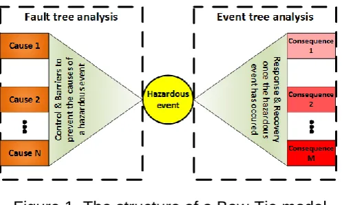
In a Bow-Tie model, a finite number of hazardous events are considered. For each of the hazardous event, a Bow-Tie model, consisting of a fault tree6 _{and an event tree}7_, is built. The hazard under consideration is the top event in the fault tree and the initiating event in the event tree. The probabilities (or frequencies) for the basic event occurrence are usually derived from asset failure data, obtained over a long period of operation2, 8, 9_.

However, distinct features of the asset, such as the condition of the asset and its individual components, the planned operational usage, inspection and maintenance policies, are currently overlooked in the traditional Bow-Tie model. Such features can have a significant impact on risk assessment, for example, an asset that is in a good condition and maintained frequently and to a high standard will have a lower failure risk estimate than an asset that is already wearing out. However, the Bow-Tie model cannot take account of the asset condition, and the analysis can be limited.

A Petri Net model-based extension to the Bow-Tie model is proposed in this paper, in order to accommodate asset specific features, where a Petri Net simulation model is built to replicate the operation and maintenance of the asset. Detailed information about the condition of the asset (for example, obtained from a condition monitoring tool), underlying degradation processes, and asset maintenance and operation strategy can be used to simulate possible outcomes of asset operation. Statistics on asset performance, obtained from the simulations, such as the frequency of failures, can then be used as inputs to the Bow-Tie model to perform risk assessment. This paper demonstrates the proposed methodology and its application to a case study of an underground passenger lift.

The paper is structured in the following way: a Bow-Tie model is presented in section 2 and the basics of the Petri Net model and proposed extensions are given in section 3. The steps of the proposed methodology are given in section 4, which are illustrated in the application of the proposed methodology to a passenger lift in section 5, followed by the conclusions and future work in section 6.

2 Bow-Tie model

Figure 1. The structure of a Bow-Tie model

2.1 Fault tree analysis

Fault tree analysis10 _{is a common technique used to estimate the probability or} frequency of a certain hazard event occurring. It is commonly used in practice by exploiting Boolean algebra to describe the logic of failure. It is a method of deductive logic, when a certain top event is chosen (e.g. a hazardous event) and the tree is developed in the branches below the selected event by answering a question “what can cause this top event”, until every branch ends with basic or undeveloped events. The diagram of the fault tree consists of two types of elements, namely gates and events. The gates in the fault tree are used to represent the Boolean operators such as AND and OR. The events usually represent failures of components and human errors. Expert knowledge about the system considered is a key factor in building a fault tree. Failure Mode and Effects Analysis (FMEA) is known as a good starting point for building a fault tree.

Once the fault tree is built, the analysis can be performed qualitatively and quantitatively. The qualitative analysis is used to define the minimal cut sets of the fault tree: a collection of basic events such that if any basic event is removed from the set the top event will not occur. Any fault tree will consist of a finite number of minimal cut sets. The quantitative analysis of the fault tree is performed to obtain the probability of the top event. The minimal cut sets can be used to calculate the probability of the top event. For small systems, the number of minimal cut sets will be relatively small, thus the top event probability can be calculated directly using the inclusion-exclusion expansion principle10_:

𝑃(𝑇) = ∑ 𝑃(𝐾𝑖)

𝑛𝑐

𝑖=1

− ∑ ∑ 𝑃(𝐾𝑖∩ 𝐾𝑗)

𝑖−1

𝑗=1 𝑛𝑐

𝑖=2

+ ⋯

+ (−1)𝑛𝑐−1𝑃(𝐾₁∩ 𝐾₂∩ … ∩ 𝐾_𝑛 𝑐),

1

where 𝑃(𝑇) is the top event probability, 𝑃(𝐾𝑖) is the probability that 𝑖th minimal cut set occurs, 𝑛𝑐 is a number of minimal cut sets, 𝐾𝑖, 𝑖 = 1, … , 𝑛𝑐 is the 𝑖th minimal cut set. Alternatively, especially for large systems, the method of Binary Decision Diagrams is commonly used to obtain the top event probability, and the derivation of minimal cut sets is not required.

𝑤𝑆𝑌𝑆(𝑡) = ∑ 𝐺𝑖(𝒒(𝑡))𝑤𝑖 𝑛

𝑖=1

(𝑡) 2

Where n is the number basic events, Gi(q(t)) is the criticality function (Birnbaum’s measure

of importance) for basic event i, and wi(t) is the frequency of basic event i. 10

Once the frequency of a hazardous event is estimated using the fault tree, the result can be further used in the event tree analysis, which is presented next.

2.2 Event tree analysis

Event tree analysis11 _{is a commonly used technique to assess the consequences of} the hazardous event. Following an initiating event, a series of possible outcomes is considered in a graphical representation. It is assumed that if an event occurs, there are only a finite number of possible outcomes, for example, failure or success. The outcomes of each event in the event tree are quantitatively measured by probabilities assigned to them, which have to sum up to 1.

For example, if the event outcome after the initiating event is success, the consequences to the system would be minimal or none, compared to the case if the second event results in a failure. The next event in the event tree is considered until the end state of the event tree is reached. The end states usually have numerical or linguistic values of accumulated consequences of all the outcomes of the previous events that lead to a particular end state of the event tree. Since each event has its predefined probability, an overall path probability can be calculated as the product of the event probabilities occurring in the selected path, multiplied by the frequency of the initiating event, obtained from the fault tree. The risk of a selected end state of the event tree is then simply the product of the consequences and the path probability11_:

𝑅𝑖𝑠𝑘𝑖 = 𝑃𝑖× 𝐶𝑖, 3

where 𝑅𝑖𝑠𝑘_𝑖 is the risk of the end state 𝑖, 𝑃_𝑖 is the path probability to reach the end state 𝑖 and 𝐶_𝑖 are the consequences of the end state 𝑖.

The biggest limitation of the Bow-Tie model is that it does not capture the change state of the system over time. It relies on the statistics of failures collected over time and doesn’t take into account other factors such as local features of the asset (e.g. frequency of usage), inspection and maintenance regimes or the current health state of the asset. Thus, a Petri Net simulation model is proposed in this paper as an extension to the Bow-Tie model to overcome these limitations, and the basics of the Petri Net model are discussed next.

3 Petri Net model

Figure 2. Graphical representation of Petri Net

A place in the PN is commonly used to represent a state or condition of the system and it can be marked with a token (or several tokens) to represent a particular condition that the system currently resides in. The tokens are removed from one place and put into another place through the use of transitions (transition firing) to mimic the change of the state.

In order for the token to move from one place to another, the transition in between the two places has to be enabled first. The transition is enabled when all input places to the transition contain the amount of tokens that is equal to the multiplicity (or weight) of the arc (usually the multiplicity is one, but a higher multiplicity can also be considered). Note that an inhibitor arc can prevent the transition to be enabled. These arcs are represented with an empty circle at the end of the arc (as shown in Figure 3). Once the transition is enabled, a delay time to fire is randomly generated (from an underlying distribution assigned to that particular transition). Once the delay time runs out, the transition is fired if all of the tokens are still present in the enabling input places. Note that the delay time can also be constant, as well as equal to 0.

When the transition fires, a token (or several tokens, depending on the multiplicity (weight) of the arc) is removed from each input place, and one token (or several tokens, depending on the multiplicity of the arc) is deposited to each output place. This way the changing state of the system can be modelled through discrete events to capture its dynamics.

Several specific arcs (see Figure 3) and transitions (see Figure 4) are introduced in this study and they are discussed next.

Figure 3. Graphical representation of arcs

T_

ID

P_ID1

Place _Transition

Arc

P_ID2 Place

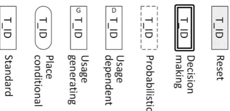
Figure 4. Graphical representation of transitions

3.1 Place conditional transition

The place conditional transition13 _{changes its delay time distribution depending on the} amount of tokens present in the input place. It is represented by a rounded corner rectangle, as shown in Figure 4. For example, the place conditional transition is useful, when modelling events that happen with different frequency depending on certain conditions, such as the lift usage during the peak hours and the off-peak hours. Instead of using many traditional transitions with different time distributions, all of the changing distributions are kept within one place conditional transition. This helps to reduce the size of the PN (since only one transition is checked whether it is enabled or not), as well as it gives a clearer graphical representation.

3.2 Usage generating transition

A novel type of transition, the usage generating transition, is introduced in this paper. Usually components degrade with usage but not with time (or the degradation with time is insignificant when compared to usage), such as mean distance to failure, mean kilometres to failure, etc. In order for the transition to fire according to usage, an additional simulation clock is implemented in this study, which is only advanced when the usage generating transitions are enabled. It is represented as the standard transition with letter “G” at the top of transition box, as shown in Figure 4.

3.3 Usage dependent transitions

Another novel type of transition is the usage dependent transition, which is linked to the usage generating transition. The time to fire for the usage dependent transitions is only reduced when usage generating transitions are enabled at the time which follows the additional simulation clock, as mentioned above. It is represented as the standard transition with letter “D” at the top of transition box, as given in Figure 4. For example, in this way the usage of the asset, not the calendar time, influences the rate of degradation.

3.4 Probabilistic transition and arcs

Figure 3. In this study, the probabilistic transitions and arcs are used to model imperfect inspection and maintenance.

3.5 Decision making transition

The decision making transition13 _{is used to adjust the amount of tokens to a defined} number in specified places, if the predefined conditions are true when the transition is firing. It also puts a token in each of the output places, as in using a standard transition. Graphically, it is represented by a rectangle with double line border in the Petri Net, as shown in Figure 4. It is used for reducing the number of traditional transitions in the Petri Net, when under certain conditions the token amount in a number of places has to be changed.

3.6 Reset transition

The reset transition13 _{resets the number of tokens in the specified places to their initial} marking and it also puts a token in each of the output places, as when a standard transition fires. It is represented by a rectangle with leaning line patterned fill, as shown in Figure 4.

In the next section, the proposed methodology is introduced by showing how the Petri Net and the non-standard transitions and arcs help to model the behaviour of the system and its processes, such as inspection and maintenance. The outputs from the PN model are then used in the Bow-Tie model to estimate the risk of hazardous events.

4 Proposed methodology

The proposed methodology is based on the development of the Petri Net model, the Monte Carlo simulations and the usage of the gathered statistics from the simulations in the Bow-Tie model. Firstly, the Petri Net model is built to represent the current condition of the asset, the deterioration profile of the asset and its components, the operation and maintenance activities. Secondly, the developed Petri Net model is simulated using Monte Carlo simulation framework to obtain statistics of the modelled asset performance over a selected time window. Finally, the Bow-Tie model is used to propagate the results of the Petri Net model in risk assessment.

In this way, the current condition of the asset, as well as other distinct features of the asset, can be taken into account when using a well-known approach of the Bow-Tie model to assess risks in operating the asset. The proposed methodology is split into several steps, which are presented next.

4.1 Main steps of the methodology

Step 1. Gather and analyse the information available about an asset, such as its description, failure and maintenance records, patterns of operational usage. Such information is also needed for the individual components of the asset. Step 2. Build a Bow-Tie model for a hazardous event, consisting of a fault tree

Step 3. Build a Petri Net model using the asset information obtained in the first step, as well as considering what outputs are going to be necessary for the Bow-Tie model, developed in the second step. The Petri Net model can describe the following features: the daily operation, degradation, catalectic failures, inspection and maintenance regimes and the related human errors. Step 4. Simulate Petri Net using the Monte Carlo simulation technique to obtain

the predictions about the performance, such as the frequency of failure occurrence of individual component and of the initiating event.

Step 5. Plug outputs of the Petri Net model, such as the frequency of the initiating event, into the Bow-Tie model to get risk estimates of the chosen hazardous event.

Note, that the focus of this paper is the Petri Net development (Step 3), therefore, in the following sections some of the other steps of the methodology are omitted or explained in less detail. The core of the methodology is presented in another work by authors15_{, however the methodology in this paper is extended by adding usage based} degradation and evidence entering in the Petri Net, which are overviewed in the following sections. Key advantages of using the Petri Net model as part of the Bow-Tie model are explained next.

4.2 Petri Net advantages over the traditional Bow-Tie model

In this section, the key improvements of using the Petri Net as an extension to the Bow-Tie model are discussed.

4.2.1 Condition based risk prognostics estimate

One of the aims of this study is to show how the actual condition of the asset and its components can be taken into account when considering risk prognostics. Information about the asset condition can be obtained from automated condition monitoring solutions, visual inspection or expert knowledge. This information is then fed into the Petri Net, by marking a certain place that corresponds to the condition of the components. In this way, evidence can be introduced in the PN model, to give a risk prognostics estimate based on the most recent information about the asset and its health. The process of entering condition evidence is illustrated in section 5.3.2.

4.2.2 Selecting a time window for the risk prognostics

Another important feature of the PN-based Bow-Tie model is that risk prognostics estimate can be obtained for various time scales. The structure of the Bow-Tie model remains the same, and only the PN model has to be simulated for different time horizons. This feature makes the methodology flexible to perform short-term (days) and longer term (months and years) risk prognostics. Therefore it can be used as an information tool for maintenance engineers to plan next maintenance works in the short term, as well as forecasting long-term estimates, which would be suitable for developing asset management strategies.

4.2.3 Usage based degradation

if it is known that a certain component has a lifetime of 10000 hours of usage, a more accurate prediction of failure due to usage can be performed when usage patterns are known. This especially holds for the components that incur friction, stress loading or other irreversible processes, that affect component degradation due to usage. Usage based degradation is illustrated in section 5.3.2.

4.2.4 Imperfect inspection and maintenance

One of the issues that is present during inspection and maintenance procedures is that there could be cases where the true cause of a failure is not identified during inspection and maintenance actions of an asset or its components might not improve their condition in first instance, e.g. the true root cause of failure is still present and this might lead to a repeat failure. Thus, these factors are taken into account in the Petri Net model to model imperfect inspection and maintenance with the use of probabilistic transitions and arcs, as detailed in sections 5.3.3 and 5.3.4.

4.3 Evidence entering in the Petri Net model

As discussed in section 4.2.1, one objective of this study is to show how the information about the condition of the asset and its components can be taken into account. Since the condition has to be discretised into a finite number of states, an issue arises for the short-term risk prognostics: what if when a short-term risk prognostic is made, and after sometime it has to be recalculated, but the asset or its components are still in the same discrete state as for the previous step of prognostics, i.e. the condition of asset or its components have changed, although slightly. To deal with such a situation, the truncated cumulative distribution functions are used to sample delay times for enabled transitions, as described below.

In the PN approach when transition is enabled, the delay to fire the transition is taken from a certain time distribution. In order to enter the evidence in the PN model about the component condition, this delay is sampled from a left-truncated distribution. This is achieved by considering the probability that the transition will fire after a time 𝑡2, given that current time is 𝑡1, i.e. the component has survived up to time t1 Since the transition firing times are sampled by inverting the cumulative distribution function (cdf), the truncation is performed on the selected cumulative distribution functions in the following way:

𝐹_𝐿𝑇(𝑡|𝜃, 𝑡𝐿) =

𝐹(𝑡|𝜃) − 𝐹(𝑡𝐿|𝜃)

1 − 𝐹(𝑡_𝐿|𝜃) , 4

where 𝐹_𝐿𝑇(𝑡|𝜃, 𝑡_𝑙) is the left-truncated cdf with the parameter vector 𝜃 and the left truncation constant 𝑡𝐿, 𝐹(𝑡|𝜃) is the complete cdf.

Consider a generic example for a 2-parameter Weibull cdf, which is a common distribution to model the degradation processes14_{, as shown below:}

𝐹𝑊(𝑡|𝜂, 𝛽) = 1 − exp (− (

𝑡 𝜂 )

𝛽

), 5

Using equation 5 in equation 4 gives the 2-parameter Weibull left-truncated cdf:

𝐹_𝑊𝐿𝑇(𝑡|𝜂, 𝛽, 𝑡𝐿) = 1 − exp ((

𝑡𝐿

𝜂 )

𝛽

− (𝑡 𝜂 )

𝛽

), 6

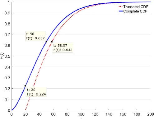
To illustrate the usage of truncated distributions, consider an example of Weibull distribution with 𝛽 = 1.5 and 𝜂 = 50. The resulting complete cdf and truncated cdf are given in Figure 5.

For a 2-parameter Weibull distribution, the parameter 𝜂 in the reliability field is referred to as a characteristic life, indicating that 63.2% of values fall below this characteristic life, e.g. in this case, there is 63.2% chance that the component has failed after 50 time units have passed. By introducing evidence, that the component lasted for 20 time units, it is now inferred that the 63.2% chance that the component has failed is at 58.07 time units (not 50), based on the resulting truncated cdf, as seen in Figure 5. This results from the fact, that given the full Weibull cdf it’s inferred that at 20 time units, there’s a chance of 22.4% that component has failed, whereas new evidence suggest that the component has survived throughout this time. This principle of using evidence about component condition is presented in section 5.3.2. This way a more accurate risk estimate that considers the actual condition of asset and its component is obtained, otherwise the risk could be underestimated.

Figure 5. Complete 𝐹𝑊(𝑡|1.5, 50) and truncated 𝐹𝑊𝐿𝑇(𝑡|1.5, 50,20) Weibull cumulative distribution functions

5 Application to a passenger lift

5.1 Asset description

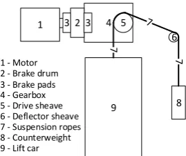
The asset considered in this study is a traction lift in an underground station, serving two levels: top landing at the street level and bottom landing at the underground train platform. The drive for a traction lift (refer to Figure 6) is provided by a motor, which operates a gearbox to turn the drive sheave. The suspension ropes are wrapped around the drive sheave and the deflector sheave, and they are connected to the counterweight and the lift car. A brake unit, consisting of a brake drum and brake pads (with brake linings attached) that are pressed against the drum, provide the braking capabilities for the lift.

Selected components of the traction lift are considered in this paper: motor, brake pads, gearbox, drive sheave and suspension ropes. Other components can also be considered as necessary, but they are out of scope of this study.

Figure 6. Simplified diagram of a traction lift

5.2 Bow-Tie model

Since the focus of this paper is to introduce the PN model, only a simple Bow-Tie model for a single hazard, such as “Lift gets stuck in between landings” is considered. The Bow-Tie model consists of a single fault tree and a single event tree. The details of the fault tree for the considered hazard are given first.

5.2.1 Fault tree for the hazard “Lift gets stuck in between landings”

The hazard “Lift gets stuck in between landings” is chosen as the top event of the fault tree (see Figure 7). It is considered to occur when the lift is in between landings and the drive for the lift gets cut off unexpectedly, which can occur due to a number of reasons, as identified from the FMEA16_{. For the purpose of this study, the following} causes are considered:

 Rope slip triggers unintended movement device, when the drive sheave wears out.

 Lift is over speeding and the overspeed governor is engaged, when either suspension ropes break or brake linings wear out.

 Gearbox fails in operation.

 Motor fails in operation.

4

9 5 1

8 6

7

7

1 - Motor

4 - Gearbox 5 - Drive sheave 6 - Deflector sheave 7 - Suspension ropes 8 - Counterweight 2 - Brake drum

2

9 - Lift car

3

Figure 7. Fault tree with a top event “Lift gets stuck in between landings”

Note, that the logic of the top event given in Figure 7 is also represented in the system failure Petri Net in section 5.3.5.

The probability of the top event is found by using an approximation of equation Error! Reference source not found., known as the rare event approximation10_:

𝑃(𝑇𝑂𝑃) ≈ 𝑃(𝐴. 𝐵) + 𝑃(𝐴. 𝐶) + 𝑃(𝐴. 𝐷) + 𝑃(𝐴. 𝐸) + 𝑃(𝐴. 𝐹), 7

where A is the event“Lift was in between landings”, B – “Drive sheave wears out”, C

– “Gearbox fails”, D – “Motor fails”, E – “Suspension ropes break”, F – “Brake linings

wear out”.

Note that the probabilities for minimal cut sets, i.e. P(A.B), P(A.C), P(A.D), P(A.E) and P(A.F) will be obtained from the system failure Petri Net (see section 5.3.5).

In addition, the rare event approximation of the frequency of the top event occurrence,

wSYS(t), is calculated, and the frequencies of each minimal cut set, 𝑤_𝐾𝑖, will be also

obtained from the system failure Petri Net:

𝑤𝑆𝑌𝑆(𝑡) ≤ ∑ 𝑤𝐾_𝑖 𝑛𝑐

𝑖=1

(𝑡) 8

5.2.2 Event tree for the hazard “Lift gets stuck in between landings”

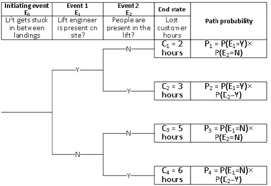
Two events are considered when building the event tree to classify the consequences for the hazard (initiating event) “Lift gets stuck in between landings”, as shown in Figure 8.

The first event considers the presence of a lift engineer on site, when the lift gets stuck. If an engineer is present, it is considered that it would take less time to deal with a hazardous situation, thus the consequences will be small. The second event considers the presence of passengers inside the lift, when the lift gets stuck in between landings. Passengers trapped in the lift would lead to more significant consequences. A

Lift gets stuck in between landings

Suspension ropes break

Lift was in between landings Drive for lift gets

cut off

Brake linings wear out Sheave

wears out

Motor fails Gearbox

fails

Overspeed governor engaged to stop overspeeding lift Rope slip triggers

combination of these two events lead to four different end states, which are expressed in terms of lost customer hours. Note that the numbers of lost customer hours are only indicative and they do not represent the actual consequences.

Figure 8. Event tree for the hazard “Lift gets stuck in between landings”

The following notation is used in Figure 8: Ci – consequence of each path i, Pi – path i probability, E0 is the initiating event, i.e. the hazard, Ej, j=1,2 are events 1 and 2, Ej = Y means that the event Ej is true, Ej = N means that the event Ej is false. Each path

probability is multiplied by the frequency of the initiating event, obtained from the Petri Net model.

The risk for the individual consequence is calculated by multiplying the value of the consequence (lost customer hours, in this particular case) by a path probability leading to the consequence. In turn, the collective risk for an initiating event (in this case, the hazard “Lift gets stuck in between landings”) is then simply a sum of risks for the individual consequences (refer to equation 3):

𝑅𝑖𝑠𝑘 = ∑ 𝑅𝑖𝑠𝑘𝑖

4

𝑖=1

, 9

where 𝑅𝑖𝑠𝑘 is the collective risk of the hazardous event “Lift gets stuck in between landings”, 𝑅𝑖𝑠𝑘_𝑖 is the risk of 𝑖th end state.

Note that the probability for people to be present in the lift and the probability for a lift engineer to be present on site are assumed in this study.

5.3 Building Petri Net model

The Petri Net model in this study describes the following processes:

 Operational usage

 Inspection

 Maintenance

 System failure

 Human error in inspecting or maintaining the asset

Note that individual PN models are built for each of the processes mentioned above, except for the human error in inspecting or maintaining the system, which is modelled in inspection and maintenance PNs.

All of these PN models are then joined into a single asset PN model, which is used in Monte Carlo simulations. The structure of the resulting PN model is shown in Figure 9. Note that the arrows in Figure 9 indicate the dependencies between the PNs. For example, once a failure occurs in a “Degradation and failure” PN it interacts with “System failure” PN, which in turn interacts with “Inspection” and “Operational” PNs.

Figure 9. Structure of a Petri Net model for a passenger lift

Due to the size of the overall PN model and the links between the individual PNs, the overall PN is not given in this paper. Instead, the individual Petri Nets that are built for each of the processes mentioned above are presented in the following sections, and the overall system PN is given in 5.3.5.

5.3.1 Lift operation

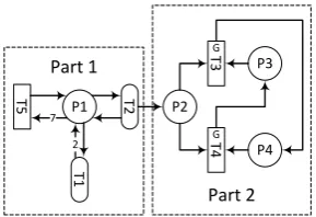
The lift, considered in this study, serves two landings: top landing at the street level, where passengers arrive to the underground station, and the bottom landing at the platform level, where underground trains are operated. The lift travels from one landing to another and it is reflected in a Petri Net to model lift usage given in Figure 10. The operational Petri Net is combined of two parts: the first part models the lift movement frequency, and the second part models the movement of lift itself.

Figure 10. Petri Net to model the operation of a lift

The frequency of lift movement is modelled using place conditional transitions T1 and T2, as introduced in section 3.1.

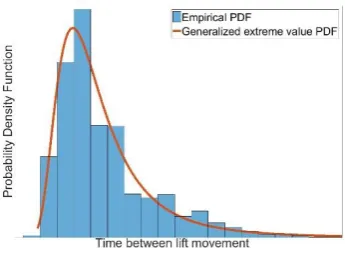
Transition T1 holds duration of the selected time intervals in a day. For example, for the morning peak time between 06:30 and 09:30, the delay time for transition T1 is set to be 180 minutes. Note that this delay time depends on the amount of tokens in place P1, as mentioned in section 3.1. In this study, 6 different time intervals are selected, based on the peak and off-peak time intervals, as used for Oyster cards pricing17_. Transition T2 holds the frequency of lift movements for each selected time interval. The time distributions for transition T2 are obtained from the accelerometer data that is collected by a monitoring solution installed in one of the lift cars in-service in a station owned by London Underground. An illustration of the time distribution for T2 is given in Figure 11.

Figure 11. Probability density function of lift movement frequency

Once the transition T2 fires, it initiates the lift movement by putting a token in place P2. If the lift is in the top landing (a token is present in place P3), the lift is assumed to be travelling from the top landing to the bottom landing (transition T3 is enabled and fires after the time, necessary for the lift to travel between the landings). Thus a token is fired from places P2 and P3 and put in place P4, indicating that the lift arrives at the bottom landing. If there is a token in place P2, the lift is assumed to be in between the landings. The lift journey from the bottom to the top landing follows the same logic. Note that transitions T3 and T4 are usage generating transitions, as introduced in 3.2. These transitions are used to advance the simulation clock that drives the usage dependent degradation.

Transition T5 is used to adjust the number of tokens in place P1, at the end of the simulated day. As mentioned before, 6 time intervals are used to model the lift usage frequency, thus if there are 7 tokens present in place P1, transition T5 fires to set the amount of tokens in place P1 to 1 (the multiplicity of arc, connecting place P1 and transition T5, is 7).

5.3.2 Degradation and failure of components

The states of the critical components, defined by London Underground engineers, are used to build the degradation and failure PN models. Two types of the PN models were developed:

 For wearing out components with catalectic failures (gearbox, motor).

 For wearing out components without catalectic failures (drive sheave, brake linings, suspension ropes).

All of the components are modelled in the same way in the proposed methodology:

 A finite number of the degradation states for a component is selected.

 Component is continuously going through states of degradation with usage or time before it fails.

In addition, for the components with catalectic failures:

 A catalectic failure can take the component to a failed state instantly.

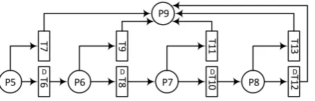
A PN model for a component with catalectic failures is presented first. Consider a gearbox that can reside in one of the following states (each state is represented with a place in the PN, see Figure 12): as good as new (P5), worn with normal noise (P6), worn with unusual noise (P7), requires urgent attention (P8), failed (P9).

Figure 12. Degradation and failure Petri Net for a gearbox (component with catalectic failures)

The gearbox is assumed to be degrading (e.g. bearings are wearing out) with usage, for example, going from state 1 (place P5) to state 2 (place P6) using transition T6, which is usage dependent, as explained in section 3.3. There is also a probability of catalectic failure (going straight to state 5 (transitions T7, T9, T11 or T13 firing)), which can occur whilst being in any of the first four states.

The degradation and failure PN model for a component without catalectic failures is presented next. Consider a drive sheave (refer to Figure 13) with the following states: as good as new (P20), worn but serviceable (P21), worn groove, uneven and evident wear (P22), groove wear requires urgent replacement (P23), worn out suspension ropes slipping (P24).

Figure 13. Degradation Petri Net for a drive sheave (component without catalectic failures)

P6 P7

P9

T6D _T8D T10D T12D

T7 T9 T11

P5 P8

T13

P21 P22 P24

T26D _T27D _T28D _T29D

Note that this PN model differs from the degradation model in Figure 12. The main reason for the difference is that the drive sheave actually incurs physical damage throughout its operation; it cannot fail suddenly, but it wears out with usage. Suspension ropes are looped around the drive sheave and thus the friction between ropes and drive sheave incurs groove wear on the sheave. Thus there is no catalectic failure for this component, as in comparison to gearbox, where it can fail suddenly at any time. Note that the degradation distributions are mostly assumed for the purpose of illustration.

5.3.3 System and component inspection

The inspection PN model is used to reveal the actual condition of each component. Under normal circumstances, periodic inspections are performed. Emergency inspections are also carried out, whenever the lift is taken out of service due to a failure of any component. Inspection is assumed to be finished when the inspection of all individual components finishes. The findings of the inspection are then used to make decisions for maintenance process.

The inspection PN model is developed for the lift as a whole system and is shown in Figure 14. For each component, whose condition is modelled with the degradation and failure PN (see section 5.3.2), an individual inspection PN model is developed.

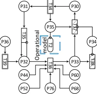
Figure 14. Inspection Petri Net for a lift (at the system level)

As mentioned before, two types of inspections can occur: scheduled inspection (place P30) and emergency inspection (place P36).

When a scheduled inspection has to start (the transition T34 fires and puts a token in place P31 “Inspection has to start” and P35 “Lift has to be out of service, planned”), the lift has to be out of service (inhibiting the transition T2 in the operational PN model in Figure 10). Once the required procedures to put the lift out of service are completed (transition T35 fires a token to a place P32), the inspection of individual components can take place (modelled in separate PN models, as in Figure 15). The inspection is finished (transition T36 fires a token to place P33), once all of the components have been inspected (tokens are present in places P44, P52, P60, P68 and P76). The lift car then can either be put back into service, if there was no corrective maintenance identified (no tokens are present in place P34), or maintenance is scheduled, and the

P30 P31

T35

P32 P33

T37

P34

T36

P35

T38

P44

P52

P60

P68 P76

P36

T39

T34

O

p

er

a

tio

n

al

m

o

d

lift is kept out of service (place P34 inhibits transitions T37 and T38) until all of the components have been rectified or replaced.

When the emergency inspection starts (a token is present in place P36) the transition T39 fires a token to place P32 after a delay (the time it takes for an engineer to start the emergency inspection). Then the inspection follows the same routine as in the case for scheduled inspection, only this time the transition T38 is fired, once the lift is put back to operation. Note, that transitions T37 and T38 are reset transitions and transitions T34 and T39 are decision making transitions.

Transition T37 is a reset transition that resets the number of tokens in places representing inspection findings when no maintenance is necessary (places P42, P50, P58, P66, P74). Transition T38 resets the number of tokens in the same places as for transition T37 and in addition for the places P80 and P81, that represent a failure of the lift, as introduced in the System failure Petri Net in section 5.3.5.

The transition T34 is a decision making transition13_{, that adjusts the amount of tokens} in the selected places that represent the fact that the lift has to be taken to one of the landings for inspection. The transition T39 performs the same thing as T34 and in addition it adjusts the amount of tokens in the selected places that represent the fact that the lift got stuck in between the landings.

Inspection models for individual components are presented next. Note that the inspection process and the PN model is identical for each type of component, considered in this study. Consider an inspection PN model for a gearbox, as given in Figure 15.

Figure 15. Inspection Petri Net for a gearbox (for the individual component) There is a revealed state of the gearbox (places P37, P38, P39, P40 and P41 in Figure 15) for each state modelled in the degradation and failure model (places P5, P6, P7, P8 and P9 in Figure 12). Hence the degradation and failure model is connected to the inspection model by using standard and probabilistic transitions and arcs. Once the inspection is finished (a token is present in place P32), the condition of the gearbox becomes revealed. Referring to the imperfect inspection, described in section 4, the probabilistic transitions and arcs are used to model human error during the inspection process, i.e. the actual condition of the component can be overlooked when

T48 T49

P40

Gearbox degradation and failure model

T40

P38 P39 P37

P6 P7 P9

P5 P8

T41 T42 T43 T44

P32

P43 P41

T47

T45 T46

P42

P44

performing the inspection. Thus, a probability to misidentify the current condition of the component is considered (probabilistic transitions T40, T41, T41, T42 and T43), except for the failed state (standard transition T44 to a place P41), where it is assumed that the failure will be revealed during the inspection with the probability of 100%. For example, when the condition of the gearbox is “Worn with unusual noise” (place P7), it is assumed that there is a 98% chance of correctly identifying this particular condition (transition T42 fires a token to place P39), a 1% chance to misidentify the current condition as a better one (“Worn with usual noise”, transition T42 fires a token to place P38) and a 1% chance to misidentify the condition as a worse one (“Gearbox requires urgent attention”, transition T42 fires a token to place P40). Note that this data has been assumed for illustration. The ordinary arcs from T42 help to keep track of the actual condition of the gearbox (back to P7) and the process of inspection (back to P32).

The findings from the inspection suggest the following actions: no maintenance is required (place P42,) or corrective maintenance is necessary (place P43). In the latter case a token is put in place P34 (see Figure 15), which counts the number of components that are in need of maintenance. This information is then used in the maintenance model, which is presented next.

5.3.4 Maintenance and replacement of components

After the inspection (scheduled and emergency) each component is maintained if necessary, and the condition is restored to an improved state, depending on the maintenance policy. Two types of maintenance PN model are developed:

 Component (gearbox, motor) repair. Condition generally improves, but not necessarily to as good as new. Repair is performed after a failure or worst degraded condition is found.

 Component (brake linings, drive sheave, suspension ropes) replacement with a new component. Component replacement is performed after a failure or worst degraded condition is found.

Figure 16. Maintenance Petri Net for a gearbox (on the left hand side, repairable component) and drive sheave (on the right hand side, component replacement) Whenever a need for maintenance has been identified (a token is present in place P43) after the inspection (no tokens in place P32 inhibiting transition T90), the maintenance is scheduled (transition T90 becomes enabled). The maintenance starts (a token is fired into place P77), when the time to prepare for the maintenance elapses (delay time of transition T90 runs out). Depending on the actual condition of the gearbox one of the transitions T91, T92 or T93 is enabled. These probabilistic transitions have individual probabilities to restore the condition of the component to a certain state. For example, transition T93 has a probability of 0.8 to fire to place P5 (maintaining the component to as good as new state), probability of 0.15 to fire to place P6 (maintaining the component to a worn state with normal noise) or probability of 0.05 to fire to place P7 (failing to maintain the component to a better state and keeping it in a worn state with unusual nose). This way, imperfect maintenance can be modelled. A similar model is built for the motor, which is also a repairable component. A maintenance PN model for a component that is replaced rather than repaired (e.g. drive sheave) is presented next. It is very similar to a PN model for a repairable component, however after the replacement the condition is improved to as good as new, so the standard transitions are used instead of probabilistic, as seen on the right hand side of Figure 16. Similar models are built for other components that are replaced.

5.3.5 System failure

The failure logic comes from the fault tree developed in section 5.2.1. The lift fails if any of its component fail. The system failure PN model (see Figure 17) is connected to each of the degradation and failure models via the places that represent failures of the critical components (place P9 for gearbox, place P14 for motor, place P19 for brake linings, place P24 for drive sheave and place P29 for suspension ropes).

Drive sheave degradation and failure model

P22 P24

P20 P23

P67 P32

T1

0

2

P79

T1

0

3

T1

0

4

T1

0

5

P34

Inspection model Gearbox degradation and failure model

P6 P7 P9

P5 P8

P43 P32

T9

0

P77

T9

1

T9

2

T9

3

P34

Figure 17. System failure Petri Net for a lift

Any failure of the critical components will put the lift out of service (a token is fired to place P80). If the lift was between the landings (token is present in place P2), a token is fired into place P81 to indicate that the lift gets stuck between the landings. In that case, an emergency inspection is requested (a token is placed in place P36) at the same time, as the lift goes out of service. Transition T2 in the operational model (see Figure 10) is inhibited in order to prevent the operation of the lift.

The marking of places P9, P14, P19, P24, P29 and P81 are observed throughout the Monte Carlo simulations to obtain the statistics necessary for the Fault tree analysis. When tokens are present in any of the places P9, P14, P19, P24 or P29 in a conjunction with a token present in a place P81, it is assumed that the minimal cut set for a top event of a fault tree, considered in this study (refer to section 5.2.1), has occurred.

5.4 Monte Carlo simulation of Petri Net model

In this section, three example scenarios are considered to illustrate how the developed PN model can be used in the Bow-Tie, in particular to carry out short-term risk prognostics. In order to show how the newly proposed PN extension of the Bow-Tie model is better than the traditional approach, the example scenarios focus on incorporating the knowledge of component condition in the predictions. Such information can come from the visual inspection or condition monitoring solutions, which are becoming commonly used on such systems as lifts19_{. Results from such} analysis can be used by maintenance engineers, for example to prioritise the maintenance of assets based on risk level or to extend the maintenance free period if an asset has a very low risk to fail.

Note that in this study, the fault trees and event trees are simple, as they are only used for illustrative purposes. The main outputs from PN models are used to determine the frequency of occurrence of minimal cut sets of the fault tree, as described in section 5.2.1, which are used to calculate the frequency of a top event as given by equation 8. No outputs from the PN model are used in the event tree, it is simply assumed that the probability for a lift engineer to be present on site is 0.6, and for the passengers to be present in the lift is 0.8. The branch probabilities, in combination with the frequency of the top event, are used to determine the risk of the hazardous event, as detailed in section 5.2.2. If the branches of the event tree need to be modelled in more detail,

P9 P14 P19 P24 P29

P2 P81

T1

1

0

T1

1

1

T1

1

2

T1

1

3

T1

1

4

P80

T1

1

5

P36

Operational model

Inspection model Degradation and failure models

their occurrence frequencies can also be expressed through simulations, however, this is out of scope of this study. The parameters are the same for all of the scenarios and are given in Table 1. A bespoke C++ software was developed to perform Monte Carlo simulations of the developed PN model.

Table 1. Parameters for Monte Carlo simulation

Number of simulations 10000

Start time of the day Start of the service, 05:30

Duration of one simulation 30 days

Frequency of scheduled inspection 20 days

In the scenarios, the condition of each component is represented by a number between 1 and 5, where 1 means that the component is in the new state, whilst 5 means that a component is in the failed state. The condition of each component for each scenario is summarised in Table 2. Note that a star (symbol *) in the table means that the time spent in the marked condition is entered into the Petri Net as evidence, as described in section 4.3. Evidence is entered with a 4-day step, starting with 0 days (corresponding to no evidence entered) until 28 days spent in a selected condition. Three scenarios are described below:

 Drive sheave is in poor condition (4) (evidence about the time spent in that condition is available), whereas other components are in minor deteriorated state (2). Delay times to move from a poor condition to a failed condition are distributed by a two parameter Weibull distribution: Weibull(β=2, η=14400). Note that η is expressed in minutes, which gives 10 days, however since this transition time depends on the usage, it’s actually 10 days of actual usage of the lift.

 Gearbox (evidence about the time spent in the condition is unavailable) and drive sheave (evidence about the time spent in the condition is available) are in poor condition.

 Gearbox (evidence about the time spent in the condition is available) and drive sheave (evidence about the time spent in the condition is available) are in poor condition.

Table 2. Conditions of different components for selected scenarios

Scenario #1 #2 #3

Gearbox condition 2 4 4*

Motor condition 2 2 2

Brake linings condition 2 2 2 Drive sheave condition 4* 4* 4* Suspension rope condition 2 2 2

5.4.1 Scenario #1

= 0 in Figure 18), the frequency of the lift getting stuck between the landings over 30 days period is around 0.16. In comparison, when the drive sheave has been in poor condition for 28 days, it increases to 0.47. Therefore, the longer the drive sheave stays in poor condition, the more likely it is for the drive sheave to fail and cause the lift getting stuck. This scenario illustrates how the unrevealed deteriorated state affects the frequency of the hazardous event. Such a situation can occur if the component quickly deteriorates from a degraded condition that still does not need maintenance, or if the next maintenance activity was not appropriately scheduled.

Note that in the simulated scenarios, the frequency curve flattens out after 20 days (on the left hand side of Figure 18). This is the time when the inspection takes place, and if the component is in poor condition it is maintained, unless the condition is overlooked during inspection. Due to this, a few failures still occur after the inspection, however, they do not significantly contribute to the overall number of failures.

Figure 18. Cumulative frequency of lift getting stuck between the landings over 30 days (on the left hand side) and component failures causing the top event (on the

right hand side) for scenario #1

In addition, it can be seen that the main cause of the top event “Lift gets stuck in between landings” is the failure of drive sheave by contributing to no less than 99.7% of occurrences, as seen on the right hand side of Figure 18. This is expected, since this is the only component in poor condition. Other causes include catalectic failures of gearbox and the motor, which are less than 0.2%. Note, that other components do not deteriorate in this short time.

Note that using fixed deterministic probabilities for the event tree branches in this study, the risk change over time will only depend on the frequency of the top event in the fault tree, thus the plots for risk profiles are not presented, since they resemble the curves seen in Figure 18. However, for completeness, an illustration of determining the risk of the hazardous event is shown next.

Consider the case, when no evidence (t = 0) and some evidence (t = 4) about the condition of the drive sheave is entered. The resulting frequencies of the top event are 0.1582/30 days and 0.2172/30 days, respectively. The path probabilities for each branch of the event tree are calculated, as shown in Figure 8, and the risk estimates are obtained, in the first case giving:

0 0.05 0.1 0.15 0.2 0.25 0.3 0.35 0.4 0.45 0.5

2 4 6 8 10 12 14 16 18 20 22 24 26 28 30

Freque

ncy

Days

t = 28 t = 24 t = 20 t = 16 t = 12 t = 8 t = 4

t = 0 0.0%

0.1% 0.2% 99.7%

99.8% 99.9%

0 4 8 12 16 20 24 28

Pr opor tio n of cau si ng top ev en t Evidence, days

𝑅𝑖𝑠𝑘 = 0.019 × 2 + 0.076 × 3 + 0.013 × 5 + 0.051 × 6 = 0.637 10

In the second case:

𝑅𝑖𝑠𝑘 = 0.026 × 2 + 0.104 × 3 + 0.017 × 5 + 0.069 × 6 = 0.863 11

This means that, when no evidence about the time spent in poor condition of the drive sheave is entered (t = 0), the risk is 0.637 lost customer hours over 30 days of lift operation, whilst the risk estimate when evidence is entered (t = 4) is 0.863 lost customer hours. This just reconfirms the fact, that omitting certain features of the asset underestimates the risk.

The results of such simulations can be useful to maintenance engineers. For example, they could set a threshold for risk (or frequency of failure) and if that threshold is violated plan, they can plan their actions appropriately. For example, if there are 7 days left until the scheduled maintenance of the asset, but the risk of failure is high over those 7 days, earlier maintenance works could be requested. Or on the contrary, if the risk is very low, the maintenance could be postponed until the asset actually needs it. This way, assets could be prioritised by their degree of risk to improve safety of asset operation and optimise their maintenance.

5.4.2 Scenario #2

In the second scenario, two components are in poor condition, so the frequency of the top event “Lift gets stuck in between landings” is higher than in scenario #1, as can be seen from Figure 19.

Figure 19. Cumulative frequency of lift getting stuck between the landings over 30 days (on the left hand side) and component failures causing the top event (on the

right hand side) for scenario #2

5.4.3 Scenario #3

In the last scenario, the evidence about both the gearbox and drive sheave condition is entered into the PN model. The cumulative frequency for the top event “Lift gets stuck in between landings” is given in Figure 20. This time the frequency increases from 0.3 to 0.73, once the corresponding evidence is entered (t = 0 and t = 28). Note that in comparison with scenario #1, the frequency has increased almost twice (from 0.16 to 0.3 and from 0.47 to 0.73).

Figure 20. Cumulative frequency of lift getting stuck between the landings over 30 days (on the left hand side) and component failures causing the top event (on the

right hand side) for scenario #3

Since the evidence for both components in poor condition is being entered, they are almost proportionally contributing to the occurrence of the top event, as can be seen from Figure 20. Once again, catalectic failures of motor contribute to the occurrence of top event with no more than 0.1%.

0.0% 0.1% 20% 30% 40% 50% 60% 70% 80%

0 4 8 12 16 20 24 28

Pr op or tio n of c au sin g top e vent Evidence, days

Gearbox failure Drive sheave failure Motor failure 0 0.1 0.2 0.3 0.4 0.5 0.6

2 4 6 8 10 12 14 16 18 20 22 24 26 28 30

Freque

ncy

Days

t = 0 t = 4 t = 8 t = 12 t = 16 t = 20 t = 24 t = 28

0.0% 0.1% 48%

50% 52%

0 4 8 12 16 20 24 28

Pr opor tio n of cau si ng top ev en t Evidence, days

Gearbox failure Drive sheave failure Motor failure 0 0.1 0.2 0.3 0.4 0.5 0.6 0.7 0.8

2 4 6 8 10 12 14 16 18 20 22 24 26 28 30

Fr

equency

Days

6 Conclusions and future work

A novel approach of using simulation within a traditional Bow-Tie framework for quantifying risk of failure for an operational asset was proposed in this study. Petri Net model with a Monte Carlo simulation framework was chosen as an extension to the Bow-Tie technique. The PN model provided several advantages over the traditional Bow-Tie model: condition-based risk prognostics for different time frames, modelling usage-based asset degradation, and considering imperfect inspection and maintenance processes.

Several extensions to the Petri Net modelling features were proposed, such as usage generating and usage dependent transitions to model the degradation of components due to usage; entering evidence about the condition of the asset, obtained from condition monitoring systems, by using truncated distributions to sample delay times. The proposed framework was illustrated on a single hazardous event for a passenger lift, for which a Bow-Tie model was developed and extended with a PN model. Several different scenarios were chosen to illustrate the effect that the condition of components have on the frequency of hazard occurrence, i.e. the lift getting stuck in between the landings. The results from the analysis of scenarios showed that the risk estimate increases with the time spent in a poor condition and ignoring the knowledge about the poor condition of an asset would lead to an underestimate of the risk (using the traditional approach), which can be misleading.

Results from such analysis could be used by maintenance engineers as a decision support tool to prioritise maintenance according to the risk levels. This would help the maintenance regime to move from corrective or scheduled maintenance to preventive or condition-based maintenance.

Further work for the proposed methodology could include other maintenance strategies, such as opportunistic maintenance. Modelling the passenger presence in the lift using a PN model, and then using its outputs in the event tree (not only the fault tree), is another potential extension to this work. Future work will also include adapting the proposed methodology to different assets, such as railway point systems and rolling stock, as a part of the PCIPP project.

Acknowledgments

References

1. Office of Rail Regulations. Common Safety Method for risk evaluation

and assessment. 2015.

2. Taig T and Hunt M. Review of LU and RSSB Safety Risk Models. 2012.

3. Wierenga PC, Lie-A-Huen L, de Rooij SE, Klazinga NS, Guchelaar H-J

and Smorenburg SM. Application of the Bow-Tie Model in Medication Safety Risk Analysis. Drug Safety. 2009; 32: 663-73.

4. Khakzad N, Khan F and Amyotte P. Dynamic risk analysis using

bow-tie approach. Reliability Engineering & System Safety. 2012; 104: 36-44.

5. Civil Aviation Authority. Bowtie templates. 2016.

6. IEC. IEC 61025 Fault Tree Analysis (FTA). 2006

7. IEC. IEC 62505 Analysis techniques for dependability – Event tree

analysis (ETA). 2010

8. Muttram RI. Railway Safety's Safety Risk Model. Proceedings of the

Institution of Mechanical Engineers, Part F: Journal of Rail and Rapid Transit. 2002; 216: 71-9.

9. Turner S, Keeley D, Glossop M and Brownless G. Review of Railway

Safety’s Safety Risk Model HSL/2002/06. 2002.

10. Andrews JD and Moss TR. Reliability and risk assessment / by J.D.

Andrews and T.R. Moss. Professional Engineering Publishing, 2002.

11. Ostrom LT and Wilhelmsen CA. Risk assessment: tools, techniques,

and their applications. John Wiley & Sons, 2012.

12. Schneeweiss WG. Petri net picture book. LiLoLe-Verlag GmbH, 2004. 13. Prescott D and Andrews J. A track ballast maintenance and inspection model for a rail network. Proceedings of the Institution of Mechanical

Engineers, Part O: Journal of Risk and Reliability. 2013; 227: 251-66.

14. Le B and Andrews J. Modelling wind turbine degradation and maintenance. Wind Energy. 2016; 19: 571-91.

15. Vileiniskis M and Remenyte-Prescott R. Extended Bow - Tie model for asset risk and reliability modelling. Application to a passenger lift. ESREL

2016. Glasgow, Scotland;2016.

16. London Underground Ltd (LUL). FMEA Traction lift. In: PCIPP project partners, (ed.). 2015.

17. Oyster and National Rail. Peak, Off Peak and Caps. 2016.

18. London Underground Ltd (LUL). Critical component checklist. In: PCIPP project partners, (ed.). 2015.