Subgraph based Classification of Explicit and Implicit Discourse Relations

Subgraph-based Classification of Explicit and Implicit

Discourse Relations

Yannick Versley SFB 833

University of T¨ubingen

[email protected]

Abstract

Current approaches to recognizing discourse relations rely on a combination of shallow, surface-based features (e.g., bigrams, word pairs), and rather specialized hand-crafted features. As a way to avoid both the shallowness of word-based representations and the lack of coverage of specialized linguistic features, we use a graph-based representation of discourse segments, which allows for a more abstract (and hence generalizable) notion of syntactic (and partially of semantic) structure. Empirical evaluation on a hand-annotated corpus of German discourse relations shows that our graph-based approach not only provides a suitable representation for the linguistic factors that are needed in disambiguating discourse relations, but also improves results over a strong state-of-the-art baseline by more accurately identifyingTemporal,ComparisonandReportingdiscourse relations.

1

Introduction

Discourse relations between textual spans capture essential structural and semantic/pragmatic aspects of text structure. Besides anaphora and referential structure, discourse relations are a key ingredient in understanding a text beyond single clauses or sentences. The automatic recognition of discourse relations is therefore an important task; approaches to the solution of this problem range from heuristic approaches that use reliable indicators (Marcu, 2000) to modern machine learning approaches such as Lin et al. (2009) that apply broad shallow features in cases without such indicators.

Especially onimplicit discourse relations, where no discourse connective could provide a reliable indication, broad, shallow features such as bigrams or word pairs conceivably lack the precision that would be needed to improve disambiguation results beyond a certain level. Conversely, hand-crafted linguistic features allow one to encode certain relevant aspects, but they have often limited coverage. Encoding detailed linguistic information in a structured representation, as in the work presented here, allows us to bridge this divide and potentially find a golden middle between linguistic precision and broad applicability.

We propose a graph-based representation of discourse segments as a way to overcome both the shal-lowness of a word-based representation and the non-specificity or lack of coverage of specialized linguis-tic features. In the rest of the paper, section 2 discusses the current state of the art in discourse relation classification. Section 3 introduces feature graphs as a general representation and learning mechanism, and section 4 provides an overview of the used corpus, as well as feature-based and graph-based repre-sentations for discourse relations. Section 5 presents empirical evaluation results.

2

Classification of Discourse Relations

In other cases, a connective can be ambiguous, as in the case of German ‘nachdem’ (as/after/since).

Nachdemcan signal multiple types of discourse relations (e.g. purely temporal or temporal and causal), as in (1):1

(1) [arg1 Nachdem sowohl das Verwaltungsgericht als auch das Oberverwaltungsgericht das Verbot best¨atigt hatten,]

[arg2rief die NPD am Freitag nachmittag das Bundesverwaltungsgericht an].

[arg1After both the Administrative Court and the Higher Administrative Court had confirmed the

interdiction,]

[arg2the NPD appealed to the Federal Administrative Court.] (Temporal+cause)

Another type of discourse relations areimplicit discourse relations, which can occur between neighbour-ing spans of text without any discourse connective signalneighbour-ing them:2

(2) [arg1Mittlerweile ist das jedoch selbstverst¨andlich]

[arg2Die gemeinsame Arbeit hilft, den anderen zu verstehen.]

[arg1In the meantime, this has become a matter of course](implied:since) (Explanation) [arg2The common work helps to appreciate the other.]

Researchers concerned with classifying the explicit discourse relations signalled by ambiguous dis-course connectives, such as Miltsakaki et al. (2005) or Pitler and Nenkova (2009), claim that a small num-ber of linguistic indicators (e.g., tense or syntactic context) can be used for successful disambiguation of discourse connectives, while Versley (2011) claims that additional semantic and structural information can help improving the classification accuracy in such cases.

In the case of implicit discourse relations, the absence of overt clues suggests that a combination of weak linguistic indicators and world knowledge is needed for successful disambiguation. Sporleder and Lascarides (2008) use positional and morphological features, as well as subsequences of words, lemmas or POS tags to disambiguate implicit relations in a reannotated subset of the RST discourse treebank (Carlson et al., 2003). Sporleder and Lascarides also show that (despite the corpus size of about 1000 examples) actual annotated relations are more useful than artificial examples derived from non-ambiguous explicit discourse relations.

Research using the implicit discourse relations annotated in the second release of the Penn Discourse Treebank (Prasad et al., 2008) shows a focus on shallow features: Pitler et al. (2009) find that the most important feature in their work on implicit discourse relations are word pairs. Lin et al. (2009) identify production rules from the constituent parse, as well as word pairs, to be the most important features in the system, with dependency triples not being useful as a features, and information from surrounding (gold-standard) discourse relations having only a minimal impact.

Most recent research, such as Feng and Hirst (2012), who classify a mixture of explicit and implicit discourse relations in the RST Discourse Treebank (Carlson et al., 2003), or Park and Cardie (2012), use these shallow features as their mainstay, adding surrounding relations and either semantic similarity (Feng and Hirst) or verb classes (Park and Cardie), leaving open the question how to incorporate more general linguistic information.

3

Feature-Node Graphs

Different information sources extract features that are relevant to subparts of an argument clause (e.g., information status and semantic class of a noun phrase), extracting features locally loses the information on each part. In contrast, we hope to maintain the information contained in these local features by representing them in feature-node graphs. This formalism also allows us to take into account more

(i)

Y r s

← X

u

a

→ Z (ii)Y ←X→a Z (iii)

r ←z _{Y →}z _s

↑

u ←z _{X →}a _Z

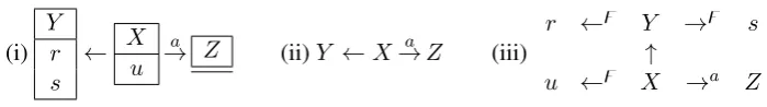
Figure 1: Example Feature-Node Graph (i), its backbone (ii), and its expansion (iii)

structure than n-grams (which are limited to relatively shallow information) or dependency triples (which would be too sparse in the case of typical discourse corpora). 3

Formally, a feature-node graph consists of a setV of vertices with labelsLV :V →L, a set of edges

E ⊆ V ×V with labelsLE : E → L, with the addition of a setF :V → P(L)that assigns to each vertex a set offeaturelabels.

Thebackboneof a feature-node graph is simply the labeled directed graph(V, LV, E, LE), without any features.

Theexpansion of a feature-node graph is the labeled directed graph(V0, L0_V, E0, L0_E)built by ex-panding the set of nodes toV0 =V ] {(v, l) ∈ V ×L|l ∈ F(v)}with labelsL0_V(v) =LV(v)for all

v∈V andL0_V((v, l)) =lfor allv ∈V, l∈F(v)and correspondingly adding edges to get the complete setE0 =E] {(v,(v, l))|l∈F(v)}, with a special symbolzfor the labels of newly introduced edges,

i.e.LE(v,(v, l)) =z.

Figure 1 gives an example of a feature-node graph with the verticesX,Y andZwithF(X) ={u},

F(Y) = {r, s}, and F(Z) = ∅, edges E = {(X, Y),(X, Z)} and edge labels LE((X, Y)) = ε,

LE((X, Z)) =a.

Representing desired information as features (instead of, e.g., using words, or POS tags, as the node labels in a dependency graph) is advantageous because that two feature-node graphs of similar structures will have a common substructure as long as the backbone of that structure is identical. In the case of words as node labels, any non-identical word would prevent the detection of the common substructure.

Machine Learning on Feature-Node Graphs Using an attributed graph representation, we can apply general substructure mining and structured learning approaches to extract good candidates for informa-tive substructures. In contrast to other fields where these approaches have been used (computational chemistry, computer vision), computational linguistics problems tend to have both larger data sets as well as larger structures. As a consequent, the na¨ıve application of these structure mining algorithms would suffer from combinatorial explosion. In particular, a star-shaped graph (i.e., the typical case of a node with a large number of features) has exponentially many substructures, which would lead to both efficiency and performance problems, while an explicit distinction between features and backbone nodes can help by explicitly or implicitly limiting the number of features that a substructure can have in order to be considered.

In general, all approaches to learn from structure fall into one of three groups: linearization ap-proaches, which decompose a structure into parts that can be presented to a linear classifier as a binary feature,structure boostingapproaches, which determine the set of included substructures as an integral part of the learning task, andkernel-based methodswhich use dynamic programming for computing the dot product in an implied vector space of substructures. Kernel-based methods on trees have been used in the re-ranking of answers in a question answering system (Moschitti and Quarteroni, 2011), whereas Kudo et al. (2004) use boosting of graphs for a sentiment task (classifying reviews into positive/negative instances). Arora et al. (2010) use subgraph features in a linearization-based approach to sentiment classification.

For simplicity reasons, we use a linearization-based approach based on subgraph mining. Generating candidate subgraphs is done using a version of gSpan (Yan and Han, 2002) that we modified to

distin-3

Relation # total # implicit % implicit % relation

Contingency

Causal

Result 133 88 66.2% 11.0%

Explanation 122 81 66.4% 10.1%

Conditional

Consequence 26 5 19.2% 0.6%

Alternation 7 2 28.6% 0.2%

Condition 13 — 0.0% —

Denial

ConcessionC 60 9 15.0% 1.1%

Concession 34 5 14.7% 0.6%

Anti-Explanation 3 3 100.0% 0.4%

Expansion

Elaboration

Restatement 149 140 94.0% 17.4%

Instance 63 39 61.9% 4.9%

Background 119 109 91.6% 13.6%

Interpretation

Summary 2 1 50.0% 0.1%

Commentary 36 28 77.8% 3.5%

Continuative

Continuation 89 71 79.8% 8.8%

Conjunction 45 1 2.2% 0.1%

Temporal

Narration 127 70 55.1% 8.7%

Precondition 34 23 67.6% 2.9%

Comparison

Parallel 55 23 41.8% 2.9%

Contrast 66 26 39.4% 3.2%

Reporting

Attribution 67 67 100.0% 8.3%

Source 65 65 100.0% 8.1%

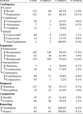
%implicit: proportion of relation instances that are implicit, rather than explicit.% rel: percentage of given relation among all implicit. About 10% of the implicit instances have multiple labels (e.g.Result+Narration).

Table 1: Frequencies of discourse relations in the corpus of Gastel et al. (2011)

guish between ‘backbone’ nodes and features, and restrict the search space to subgraphs with at most three feature nodes by stopping the expansion of a subgraph pattern whenever it exceeds this limit.

4

Disambiguating Discourse Relations

Relation # total % relation

Temporal 276 93.9%

Result situational

enable 94 31.6%

cause 65 21.7%

rhetorical

evidence 12 4.1%

speech-act 6 2.4%

Comparison

parallel 14 4.8%

contrast 16 5.8%

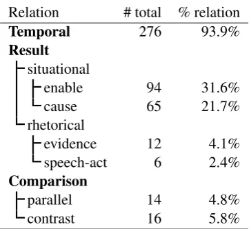
About 65% ofnachdeminstances have multiple labels.

Table 2: Frequencies of discourse relations in thenachdemdata from Simon et al. (2011)

Among the most frequent unmarked relations are Restatement and Background from the Expan-sion/Elaboration group, which predominantly occur as implicit discourse relations, as well asResultand

Explanation, which occur unmarked in about two thirds of the cases. In other cases, such as Conse-quence, Concession (is limited to cases of contraexpectation) and ConcessionC (which also includes more pragmatic concession relations), only a minority of relation instances is implicit whereas the ma-jority is marked by an explicit connective.

Relations that are typically marked, such asContrast– see example (3) – orConcession/ConcessionC

– see example (4) – often contain weak indicators for the occurring discourse relation, such as the oppo-sition policemen-demonstratorsin the first case, or the negation of a reference to Arg1 (“this wish will not be fullfilled soon”).

(3) [arg1159 Polizisten wurden verletzt.]

[arg2Zahlen ¨uber verletzte DemonstrantInnen liegen nicht vor.] (Contrast) [arg1159 policemen were injured.][arg2No data is available regarding injured demonstrators.]

(4) [arg1“Nun will ich endlich in Frieden leben.”]

[arg2Dieser Wunsch Ahmet Zeki Okcuoglus wird so bald nicht in Erf¨ullung gehen.] [arg1“Now I finally want to live in peace.”](implied: However,)

[arg2This wish of Ahmet Zeki Okcuoglu will not be fulfilled any time soon.] (ConcessionC)

Improving the performance on explicit discourse relations beyond the easiest cases, especially in the case of the notoriously ambiguous temporal connectives, is only possible by exploiting weak indicators for a relation. Features exploiting these weak indicators are a key ingredient to successfully predicting both implicit discourse relations and the non-majority readings of explicit discourse relations with ambiguous temporal connectives.

4.1 Linguistic Features

We implemented a group of specialized linguistic features, which are inspired by those that were suc-cessfully used in related literature (Sporleder and Lascarides, 2008; Pitler et al., 2009; Versley, 2011).

As implicit discourse relations can occur intra- as well as intersententially, thetopological relation between the arguments is classified by syntactic embedding (if one argument is in the pre- or post-field of the other), or as one preceding, succeeding or embedding the other.

head lemma(s) of each argument, which is normally the main verb, is also included as a feature (e.g.

1Lverletzenfor the Arg1 of example 3).

We also mark thesemantic type of adjunctspresent in either relation argument, with categories for temporal, causal, or concessive adverbials, conjunctive focus adverbs (also,as well), and commentary adverbs (doubtlessly, actually, probably . . . ). As an example, an Arg1 containing “despite the cold” would receive a feature1adj concessive.

The detection ofcotaxonomic relationsbetween words in both arguments using the German word-net GermaNet (Henrich and Hinrichs, 2010). Such pairs of contrasting lemmas, such as hot-cold or

policeman-demonstratorcommonly indicate aparallelorcontrastrelation. If two words share a com-mon hyperonym (excluding the uppermost three levels of the noun hierarchy, which are not informative enough), feature values indicating the least-common-subsumer synset (such astemperature adjective) and up to two hyperonyms are added.

A sentiment feature uses the lists of emotional words and of ‘shifting’ words (which invert the emotional value of the phrase) by Klenner et al. (2009) as well as the most reliable emotional words from Remus et al. (2010). The combination of emotional words and shifting words into a feature is similar to Pitler et al. (2009): according to the presence of positive- or negative-emotion words, each relation argument is tagged as POS,NEG orAMB. When a negator or shifting expression is present, a “-NEG” is added to the tag, yielding, e.g. “1 pol NEG-NEG” for an Arg1 phrase containing the words ‘not bad’.

4.2 Shallow Features

As mentioned in section 2, shallow lexical features empirically constitute a very important ingredient in the automatic classification of implicit (and ambiguous explicit) discourse relations, despite the fact that they lack most – semantic or structural – generalization capabilities. We implemented three groups of features that have been identified as important in the prior work of Sporleder and Lascarides (2008), Lin et al. (2009) and Pitler et al. (2009).

A first group of features captures (unigrams and) bigrams of words, lemmas, and part-of-speech tags. In this fashion, the bigram “Zahlen ¨uber” from Arg2 of (3) would be represented by word forms

2w Zahlen ¨uber, lemmas2l Zahl ¨uberand POS tags2p NN APPR.4

Word pairs, i.e., pairs consisting of one word from each of the discourse relation arguments, have been identified as a very useful feature for the classification of implicit discourse relations in the Penn Discourse Treebank (Lin et al., 2009; Pitler et al., 2009), and, quite surprisingly, also for smaller datasets such as the discourse relations in the RST Discourse Treebank targeted by Feng and Hirst (2012) or the ambiguous connective dataset used by Versley (2011).5 Because of the morphological richness of German, we use lemma pairs across sentences; for example (3), the lemma Polizist from Arg1 and the lemma DemonstrantIn from Arg1, among others, would be combined into a feature value

wp Polizist DemonstrantIn.

Finally,CFG productionswere used by Lin et al. (2009) to capture structural information, including parallelism. Context-free grammar expansions are extracted from the subtrees of the relation arguments and used as features by marking whether the corresponding rule type occurs only in one, or in both, arguments. In example (3), the CFG rule ‘PX →APPR NX’ for prepositional phrases occurs in both arguments, yielding a feature “pr B PX=APPR-NX”, whereas the preterminal rule “APPR→ ¨uber” only occurs in Arg2 (yielding “pr 2 APPR=¨uber”).

4

Sporleder and Lascarides (2008) use a Boosting classifier (BoosTexter) that can extract and use arbitrary-length subse-quences from its training data. As our dataset is small enough that we do not expect a significant contribution from longer sequences, we approximate the sequence boosting by extracting unigrams and bigrams. As with the other shallow features, unigrams and bigrams are subject to the same supervised feature selection that is also applied to subgraph features.

5

S mod:wollen mood=i tense=s cat:SIMPX lm:leben MOD cat:ADVX cls:tmp lm:nun fd:VF ARG cat:NX gf:ON ref:old lm:ich fd:MF MOD cat:ADVX lm:endlich fd:MF MOD cat:PX lm:in arg:Frieden fd:MF S future mood=i tense=s cat:SIMPX lm:gehen ARG cat:NX gf:ON ref:mediated lm:Wunsch fd:VF MOD cat:ADVX cls:tmp lm:bald fd:MF MOD cat:ADVX lm:nicht fd:MF ARG cat:PX gf:OPP lm:in arg:Erfüllung fd:MF

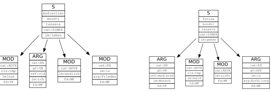
Figure 2: The complete graphs built from the implicit relation arguments “Nun will ich endlich in Frieden leben.” and “Dieser Wunsch Ahmet Zeki Okcuoglus wird so bald nicht in Erf¨ullung gehen.” – cf. ex. (4).

4.3 Graph construction

The backboneof the graph is built using nodes for a clause (S), and including children nodes for any clause adjuncts (MOD), verb arguments (ARG). In the case of relation arguments being in a (syntactic) matrix clause - subclause relationship (e.g. [arg1Peter wears his blue pullover,_{] [arg2} which he bought last year]), the graph corresponding to the matrix clause receives a special node (SUB-CL, orREL-CL

for relative clauses). This is universally the case for the explicit relations in the case ofnachdem, but may also occur in the case of unmarked relations. For example,Backgroundrelations are frequently realized by relative clauses. Non-referring noun phrases (which are tagged as ‘expletive’ or ‘inherent reflexive’ in the referential layer of T¨uBa-D/Z), receive a node labelexpletiveinstead ofARG.

In each of the adjunct/argument nodes, we includesyntactic information such as the category of the node (nominal/prepositional/adverbial phrase, e.g. cat:NXfor a noun phrase), the topological field (cf. H¨ohle, 1986, e.g. fd:MFfor a constituent occurring in the middle field) and, for clause arguments, the grammatical function (subject, accusative or dative object or predicative complement – e.g.,gf:OA

for the accusative object). Clauses nodes contain features for tense and mood based on the main and auxiliary/modal verb(s) of that clause (e.g.,mood=i,tense=sfor an indicative/past clause).

In the realm ofsemantic information, we use the heuristics of Versley (2011) to identifysemantic classes of adverbials, in particular temporal, causal or concessive adverbials, conjunctive focus adverbs, and commentary adverbs. As the backbone of our graph structure abstracts from syntactic categories and only distinguishes adjuncts and arguments, it is possible to learn generalizations over different realiza-tions of the same type of adjunct: for example, temporal adjuncts may be realized as a noun phrase (next Monday), a prepositional phrase (in the last week), an adverb (later), or a clause (when Peter was ill).

From the graph representations of relation arguments that are created in this step, frequent subgraphs are extracted. The subgraphs must occur at least five times in either the Arg1 or Arg2 graph, have at most seven nodes, of which at least two must be backbone nodes, and at most three can be feature nodes.

For the learning task, features are created by concatenating an identifier for the subgraph (e.g.

graph1234) with a suffix specifying whether it occurs only in the main clause ( 1), only in the sub-clause ( 2), or in both sub-clauses ( 12). Detecting subgraphs that occur in both sub-clauses allows the system to take into account parallelism in terms of syntactic and/or semantic properties of parts of each clause.

Both the shallow features and the subgraph features are subject tosupervised feature selection: In each fold of the 10-fold crossvalidation, the training portion is used to score each feature and only include the most informatives one in each fold. For this, an association measure between the examples from that training portion and, for each relation label, the examples in the training portion that the label occurs in, is determined. The best score over all the labels is kept, and is used to filter out features that score less than the top-N features of that group. Supervised feature selection has been used by Lin et al. (2009), using pointwise mutual information (PMI) on candidate productions and word pairs, and in the work of Arora et al. (2010) using Pearson’sχ2statistic on candidate subgraphs. We tried PMI,χ2 and the Dice coefficient 2_||_AA_||∩_BB_|| as association measures, and empirically found that the Dice coefficient worked best in the case of implicit discourse relations.

5

Evaluation Results

For both the 294 explicitnachdemrelations and the 803 implicit discourse relations, we use a 10-fold cross-validation scheme where, successively, one tenth of the data is automatically labeled by a model from the remaining nine tenth of the data. Multiple relation labels are predicted by using binary clas-sifiers (one-vs-all reduction) and using confidence values to choose one or several labels among those that have the most confident positive classification. In the case of multiple positive classifications (e.g., ifReporting,TemporalandExpansionall receive a positive classification), relations are only considered for the ‘second’ label if the most-confident label and the potential second label have been seen together in the training data (e.g. ContingencyandTemporalcan occur together, butReportingwill not be extended by a second relation labels). In a second step, the coarse grained relation label (or labels) is extended up to the finest taxonomy level (e.g., an initial coarse-grainedContingencylabel is extended to Contin-gency.Causal.Explanation). In our experiments, we use SVMperf, an SVM implementation that is able to train classifiers optimized for performance on positive instances (Joachims, 2005).

Tables 3 and 4 provide evaluation figures for different subsets of the presented features, using ag-gregate measures over relations both at the coarsest level (for implicit discourse relations, the five cate-goriesContingency,Expansion,Temporal,Comparison,Reporting), and the finest level (which contains twenty-one relations in the case of implicit relations).

For each level of granularity, we can measure the quality of the classifier’s predictions in terms of an average over relation tokens, giving partial credit for partially matching labelings (e.g., a system prediction of Narration or Narration+Comparison, instead of gold-standard Narration+Result). This measure, the dice score, assigns partial credit for a relation token when system and/or gold standard contain multiple labels and both label sets overlap, calculated as _|2_G|G_|+∩_|S_S|_| – an exact match would be scored as 1.0, whereas guessing a sub- or superset (e.g. onlyResultinstead ofResult+Narration) would give a contribution of 0.66 for that example, and overlapping predictions (Result+Comparisoninstead ofResult+Narration) would get a partial credit of 0.5. As an average over relation types, we can also calculate an average of the F-score over all relations, yielding themacro-averaged F-score(MAFS).

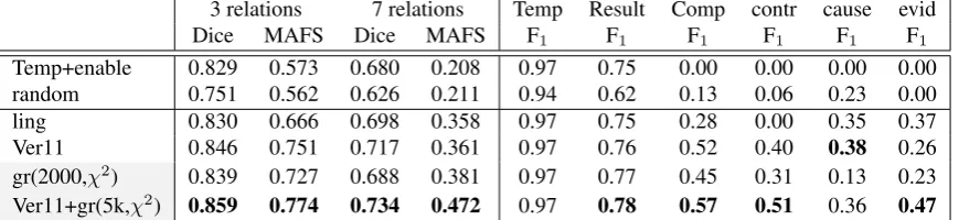
3 relations 7 relations Temp Result Comp contr cause evid Dice MAFS Dice MAFS F1 F1 F1 F1 F1 F1

Temp+enable 0.829 0.573 0.680 0.208 0.97 0.75 0.00 0.00 0.00 0.00 random 0.751 0.562 0.626 0.211 0.94 0.62 0.13 0.06 0.23 0.00 ling 0.830 0.666 0.698 0.358 0.97 0.75 0.28 0.00 0.35 0.37 Ver11 0.846 0.751 0.717 0.361 0.97 0.76 0.52 0.40 0.38 0.26 gr(2000,χ2) 0.839 0.727 0.688 0.381 0.97 0.77 0.45 0.31 0.13 0.23 Ver11+gr(5k,χ2_{) 0.859 0.774 0.734 0.472 0.97 0.78 0.57 0.51 0.36 0.47}

Table 3: Results for disambiguation of nachdem. Rows include the specialized linguistic features of Versley (2011), as ling, a system additionally using word pairs and CFG (with unsupervised feature selection), asVer11, and finally versions including the graph representation (grandVer11+gr). Shaded rows indicate variants using the graph representation.

Disambiguating nachdem For the disambiguation of the ambiguous temporal connective nachdem, we use a set of linguistic and shallow features to reproduce the results of Versley (2011), similar to that described in section 3, but with very few exceptions.6 _{Looking at the aggregate measures, we see that the} graph-based features in isolation already perform quite well, surpassing a version with linguistic features, but no word pairs or CFG productions. Adding subgraph features with appropriate feature selection to the complete system (including linguistic and shallow features) yields a further improvement over a relatively strong baseline.

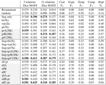
Implicit relations Table 4 presents both aggregate measures (Dice, macro-averaged F-measure) as well as scores for the most important coarse-grained relations. We provide results for the full graph (grA), a version with all features except information status (grB), and finally a minimal version that excludes all semantic features and lemmas (grC).

In general, both the linguistic features and the graph features perform much better than the shallow features (with the best single source of information being the complete graph), and also that a combina-tion of linguistic and all shallow features (all–gr) suffers from

In the second section of the table, the influence of different information sources is detailed. We see that, despite the skewed distribution of relations, all information sources outperform the most-frequent-sense baseline by themselves. By providing a higher precision on Expansionrelations, and generally better performance on Reportingrelations, the graph-based representation performs better than any of the other information sources, and is the only information source to provide enough information for the identification ofComparisonrelations. The third group of rows, showing combinations of the linguistic features with the shallow information sources and with the graph representation, shows that, while the addition of specialized features to the shallow ones yields a general improvement, the graph-based repre-sentation still works best; forTemporalrelations, we see that the noise brought in by the shallow features hinders their identification more than in the case of the graph-based representation.

The last part of table 4 provides evaluation results for a system using the complete set of information sources (all), for systems leaving out one of the shallow information sources (all–bi,all–wp,all–pr), and a system using only linguistic and shallow features but no graph information (all–gr). We see that, in general, the identification of rare relations such asTemporal,Comparison, andReportingis helped by the graph representation (the full system obtains the best MAFS scores of 0.438 and 0.208, for coarse- and fine-grained relations, respectively, against 0.388 and 0.145 for the system without graph information). System variants with graph information also obtain higher coarse-grained dice scores (0.564–0.571) than the version without graph information (0.551 forall–gr). In the same vein, we see that the parsimonious

grC graph gives the best combination result (allC–pr, including linguistic, word pair, unigram/bigram, and graph features) despite the more informativegrAgiving the best results in isolation.

6

5 relations 21 relations Cont Expn Temp Comp Rept Dice MAFS Dice MAFS F1 F1 F1 F1 F1

Restatement 0.474 0.129 0.161 0.014 0.00 0.00 0.65 0.00 0.00 random 0.338 0.233 0.096 0.056 0.06 0.27 0.50 0.21 0.14 ling only 0.540 0.396 0.274 0.127 0.40 0.68 0.32 0.00 0.58 bi(5k) 0.516 0.301 0.260 0.098 0.40 0.65 0.00 0.00 0.45 wp(2k) 0.494 0.307 0.198 0.084 0.42 0.65 0.02 0.05 0.40 pr(5k) 0.478 0.154 0.192 0.034 0.12 0.65 0.00 0.00 0.00 grA(20k) 0.559 0.381 0.269 0.163 0.39 0.69 0.24 0.00 0.59 grB(20k) 0.549 0.387 0.274 0.187 0.36 0.69 0.22 0.09 0.57 grC(20k) 0.544 0.382 0.268 0.164 0.36 0.68 0.23 0.09 0.55 ling+bi(5k) 0.545 0.399 0.300 0.141 0.39 0.69 0.33 0.00 0.59 ling+wp(2k) 0.552 0.408 0.277 0.144 0.42 0.68 0.33 0.00 0.61 ling+pr(5k) 0.546 0.399 0.297 0.142 0.40 0.68 0.33 0.00 0.58 ling+grA(20k) 0.574 0.389 0.285 0.161 0.37 0.70 0.28 0.00 0.59 ling+grB(20k) 0.579 0.394 0.294 0.173 0.36 0.71 0.30 0.00 0.60 ling+grC(20k) 0.580 0.411 0.307 0.179 0.37 0.70 0.35 0.03 0.60 all-gr 0.538 0.343 0.273 0.116 0.42 0.68 0.10 0.00 0.52 allA 0.572 0.408 0.306 0.178 0.43 0.70 0.29 0.00 0.62 allB 0.573 0.411 0.301 0.171 0.40 0.70 0.32 0.00 0.63 allC 0.579 0.422 0.309 0.177 0.38 0.70 0.35 0.04 0.65 allA-pr 0.576 0.407 0.300 0.174 0.41 0.70 0.32 0.00 0.61 allB-pr 0.581 0.410 0.298 0.171 0.40 0.70 0.32 0.00 0.62 allC-pr 0.581 0.425 0.310 0.185 0.36 0.70 0.36 0.07 0.64

Table 4: Implicit discourse relations: specialized linguistic features (ling), word/lemma/pos bigrams (bi), word pairs (wp), CFG productions (pr), and different methods for constructing graphs (grA,grB

andgrC). Shaded rows indicate variants using the graph representation.

6

Conclusion

In this article, we presented a novel way to identify discourse relations using feature-node graphs to represent rich linguistic information. We evaluated our approach on two datasets: one dataset containing implicit discourse relations and one containing explicit discourse relations with the ambiguous temporal connectivenachdem. We showed in both cases that using the graph-based representation, with appropri-ate heuristics for supervised feature selection, yields an improvement even over a strong stappropri-ate-of-the-art system using linguistic and shallow features.

Besides applying the techniques on other corpora, issues for future work would include the use of unlabeled data to improve the generalization capability of the classifier, or the use of reranking techniques to combine local decisions into a global labeling.

Acknowledgements The author is grateful to the Deutsche Forschungsgemeinschaft (DFG) for fund-ing as part of SFB 833, and to Corina Dima, Erhard Hinrichs, Emily Jamison and Verena Henrich, as well as the three anonymous reviewers, for suggestions and constructive comments on earlier versions of this paper.

References

Arora, S., E. Mayfield, C. Penstein-Ros´e, and E. Nyberg (2010). Sentiment classification using automat-ically extracted subgraph features. InNAACL 2010.

Gastel, A., S. Schulze, Y. Versley, and E. Hinrichs (2011). Annotation of implicit discourse relations in the T¨uBa-D/Z treebank. InGSCL 2011.

Henrich, V. and E. Hinrichs (2010). GernEdiT - the GermaNet editing tool. InProceedings of the Seventh Conference on International Language Resources and Evaluation (LREC 2010), pp. 2228–2235. H¨ohle, T. (1986). Der Begriff “Mittelfeld”, Anmerkungen ¨uber die Theorie der topologischen Felder. In

Akten des Siebten Internationalen Germanistenkongresses 1985, pp. 329–340.

Joachims, T. (2005). A support vector method for multivariate performance measures. In Proceedings of the International Conference on Machine Learning (ICML).

Klenner, M., S. Petrakis, and A. Fahrni (2009). Robust compositional polarity classification. InRecent Advances in Natural Language Processing (RANLP 2009).

Kudo, T., E. Maeda, and Y. Matsumoto (2004). An application of boosting to graph classification. In

NIPS 2004.

Lin, Z., M.-Y. Kan, and H. T. Ng (2009). Recognizing implicit discourse relations in the Penn Discourse Treebank. InEMNLP 2009.

Marcu, D. (2000). The rhetorical parsing of unrestricted texts: A surface-based approach.Computational Linguistics 26, 3.

Miltsakaki, E., N. Dinesh, R. Prasad, A. Joshi, and B. Webber (2005). Experiments on sense annotations and sense disambiguation of discourse connectives. InTLT 2005.

Moschitti, A. and S. Quarteroni (2011). Linguistic kernels for answer re-ranking in question answering systems.Information Processing and Management 47, 825–842.

Park, J. and C. Cardie (2012). Improving implicit discourse relation recognition through feature set optimization. InSIGDIAL 2012, pp. 108–112.

Pasch, R., U. Brauße, E. Breindl, and U. H. Waßner (2003). Handbuch der deutschen Konnektoren. Berlin / New York: Walter de Gruyter.

Pitler, E., A. Louis, and A. Nenkova (2009). Automatic sense prediction for implicit discourse relations in text. InACL-IJCNLP 2009.

Pitler, E. and A. Nenkova (2009). Using syntax to disambiguate explicit discourse connectives in text. InACL 2009 short papers.

Prasad, R., N. Dinesh, A. Lee, E. Miltsakaki, L. Robaldo, A. Joshi, and B. Webber (2008). The Penn Discourse Treebank 2.0. InProceedings of LREC 2008.

Remus, R., U. Quasthoff, and G. Heyer (2010). SentiWS — a publicly available German-language resource for sentiment analysis. InProceedings of LREC 2010.

Simon, S., E. Hinrichs, S. Schulze, and Y. Versley (2011). Handbuch zur Annotation expliziter und impliziter Diskursrelationen im Korpus der T¨ubinger Baumbank des Deutschen (T¨uBa-D/Z) Teil I: Diskurskonnektoren. Technical report, Seminar f¨ur Sprachwissenschaft, Universit¨at T¨ubingen.

Sporleder, C. and A. Lascarides (2008). Using automatically labelled examples to classify rhetorical relations: An assessment.Natural Language Engineering 14(3), 369–416.

Versley, Y. (2006). A constraint-based approach to noun phrase coreference resolution in German news-paper text. InKonferenz zur Verarbeitung Nat¨urlicher Sprache (KONVENS 2006).

Versley, Y. (2011). Multilabel tagging of discourse relations in ambiguous temporal connectives. In

Proceedings of Recent Advances in Natural Language Processing (RANLP 2011).