Proceedings of SIGDIAL 2010: the 11th Annual Meeting of the Special Interest Group on Discourse and Dialogue, pages 107–115,
Sparse Approximate Dynamic Programming for Dialog Management
Senthilkumar Chandramohan, Matthieu Geist, Olivier Pietquin SUPELEC - IMS Research Group, Metz - France.
{senthilkumar.chandramohan, matthieu.geist, olivier.pietquin}@supelec.fr
Abstract
Spoken dialogue management strategy op-timization by means of Reinforcement Learning (RL) is now part of the state of the art. Yet, there is still a clear mis-match between the complexity implied by the required naturalness of dialogue sys-tems and the inability of standard RL al-gorithms to scale up. Another issue is the sparsity of the data available for training in the dialogue domain which can not ensure convergence of most of RL algorithms. In this paper, we propose to combine a sample-efficient generalization framework for RL with a feature selection algorithm for the learning of an optimal spoken dia-logue management strategy.
1 Introduction
Optimization of dialogue management strategies by means of Reinforcement Learning (RL) (Sut-ton and Barto, 1998) is now part of the state of the art in the research area of Spoken Dialogue Systems (SDS) (Levin and Pieraccini, 1998; Singh et al., 1999; Pietquin and Dutoit, 2006; Williams and Young, 2007). It consists in casting the dia-logue management problem into the Markov Deci-sion Processes (MDP) paradigm (Bellman, 1957) and solving the associated optimization problem. Yet, there is still a clear mismatch between the complexity implied by the required naturalness of the dialogue systems and the inability of standard RL algorithms to scale up. Another issue is the sparsity of the data available for training in the dialogue domain because collecting and annotat-ing data is very time consumannotat-ing. Yet, RL algo-rithms are very data demanding and low amounts of data can not ensure convergence of most of RL algorithms. This latter problem has been ex-tensively studied in the recent years and is ad-dressed by simulating new dialogues thanks to
a statistical model of human-machine interaction (Pietquin, 2005) and user modeling (Eckert et al., 1997; Pietquin and Dutoit, 2006; Schatzmann et al., 2006). However, this results in a variability of the learned strategy depending on the user model-ing method (Schatzmann et al., 2005) and no com-mon agreement exists on the best user model.
The former problem, that is dealing with com-plex dialogue systems within the RL framework, has received much less attention. Although some works can be found in the SDS literature it is far from taking advantage of the large amount of ma-chine learning literature devoted to this problem. In (Williams and Young, 2005), the authors reduce the complexity of the problem (which is actually a Partially Observable MDP) by automatically con-densing the continuous state space in a so-called
summary space. This results in a clustering of the state space in a discrete set of states on which stan-dard RL algorithms are applied. In (Henderson et al., 2008), the authors use a linear approximation scheme and apply the SARSA(λ) algorithm (Sut-ton and Barto, 1998) in a batch setting (from data and not from interactions or simulations). This al-gorithm was actually designed for online learning and is known to converge very slowly. It there-fore requires a lot of data and especially in large state spaces. Moreover, the choice of the features used for the linear approximation is particularly simple since features are the state variables them-selves. The approximated function can therefore not be more complex than an hyper-plane in the state variables space. This drawback is shared by the approach of (Li et al., 2009) where a batch al-gorithm (Least Square Policy Iteration or LSPI) is combined to a pruning method to only keep the most meaningful features. In addition the com-plexity of LSPI isO(p3).
data sparsity problem is also widely addressed in this literature, and sample-efficiency is one main trend of research in this field. In this paper, we propose to combine a sample-efficient batch RL algorithm (namely the Fitted Value Iteration (FVI) algorithm) with a feature selection method in a novel manner and to apply this original combi-nation to the learning of an optimal spoken dia-logue strategy. Although the algorithm uses a lin-ear combination of features (or basis functions), these features are much richer in their ability of representing complex functions.
The ultimate goal of this research is to provide a way of learning optimal dialogue policies for a large set of situations from a small and fixed set of annotated data in a tractable way.
The rest of this paper is structured as follows. Section 2 gives a formal insight of MDP and briefly reminds the casting of the dialogue prob-lem into the MDP framework. Section 3.2 pro-vides a description of approximate Dynamic Pro-gramming along with LSPI and FVI algorithms. Section 4 provides an overview on how LSPI and FVI can be combined with a feature selection scheme (which is employed to learn the represen-tation of theQ-function from the dialogue corpus). Our experimental set-up, results and a comparison with state-of-the-art methods are presented in Sec-tion 5. Eventually, SecSec-tion 6 concludes.
2 Markov Decision Processes
The MDP (Puterman, 1994) framework is used to describe and solve sequential decision mak-ing problems or equivalently optimal control prob-lems in the case of stochastic dynamic systems. An MDP is formally a tuple{S, A, P, R, γ}where
S is the (finite) state space, A the (finite) action space, P ∈ P(S)S×A the family of Markovian transition probabilities1,R∈RS×A×Sthe reward
function andγthe discounting factor (0≤γ ≤1). According to this formalism, a system to be con-trolled steps from state to state (s∈S) according to transition probabilities P as a consequence of the controller’s actions (a ∈ A). After each tran-sition, the system generates an immediate reward (r) according to its reward function R. How the system is controlled is modeled with a so-called
policy π ∈ AS mapping states to actions. The quality of a policy is quantified by the so-called value function which maps each state to the
ex-1Notationf∈ABis equivalent tof:B→A
pected discounted cumulative reward given that the agent starts in this state and follows the policy
π:Vπ(s) =E[P∞
i=0γiri|s0 =s, π]. An optimal policyπ∗ maximizes this function for each state:
π∗= argmaxπVπ. Suppose that we are given the optimal value functionV∗(that is the value func-tion associated to an optimal policy), deriving the associated policy would require to know the transi-tion probabilitiesP. Yet, this is usually unknown. This is why the state-action value (orQ-) function is introduced. It adds a degree of freedom on the choice of the first action:
Qπ(s, a) =E[ ∞
X
i=0
γiri|s0 =s, a0 =a, π] (1)
The optimal policy is noted π∗ and the related
Q-functionQ∗(s, a). An action-selection strategy that is greedy according to this function (π(s) = argmaxaQ∗(s, a)) provides an optimal policy.
2.1 Dialogue as an MDP
The casting of the spoken dialogue management problem into the MDP framework (MDP-SDS) comes from the equivalence of this problem to a sequential decision making problem. Indeed, the role of the dialogue manager (or the decision maker) is to select and perform dialogue acts (ac-tions in the MDP paradigm) when it reaches a given dialogue turn (state in the MDP paradigm) while interacting with a human user. There can be several types of system dialogue acts. For example, in the case of a restaurant information system, possible acts are request(cuisine type),
provide(address),confirm(price range),close etc.
The dialogue state is usually represented effi-ciently by the Information State paradigm (Lars-son and Traum, 2000). In this paradigm, the di-alogue state contains a compact representation of the history of the dialogue in terms of system acts and its subsequent user responses (user acts). It summarizes the information exchanged between the user and the system until the considered state is reached.
reward is usually approximated by a linear com-bination of objective measures like dialogue dura-tion, number of ASR errors, task completionetc. (Walker et al., 1997).
3 Solving MDPs
3.1 Dynamic Programming
Dynamic programming (DP) (Bellman, 1957) aims at computing the optimal policy π∗ if the transition probabilities and the reward function are known.
First, the policy iteration algorithm computes the optimal policy in an iterative way. The ini-tial policy is arbitrary set toπ0. At iterationk, the policyπk−1 is evaluated, that is the associatedQ -functionQπk−1(s, a) is computed. To do so, the Markovian property of the transition probabilities is used to rewrite Equation (1) as :
Qπ(s, a) =Es0|s,a[R(s, a, s0) +γQπ(s0, π(s0))]
=TπQπ(s, a) (2)
This is the so-called Bellman evaluation equa-tion and Tπ is the Bellman evaluation opera-tor. Tπ is linear and therefore this defines a lin-ear system that can be solved by standard meth-ods or by an iterative method using the fact that Qπ is the unique fixed-point of the Bell-man evaluation operator (Tπ being a contrac-tion): Qˆπi = TπQˆπi−1, ∀Qˆπ0 limi→∞Qˆπi =
Qπ. Then the policy is improved, that is
πk is greedy respectively to Qπk−1: πk(s) = argmaxa∈AQπk−1(s, a). Evaluation and im-provement steps are iterated until convergence of
πktoπ∗(which can be demonstrated to happen in a finite number of iterations whenπk=πk−1).
The value iteration algorithm aims at estimat-ing directly the optimal state-action value function
Q∗which is the solution of the Bellman optimality equation (or equivalently the unique fixed-point of the Bellman optimality operatorT∗):
Q∗(s, a) =Es0|s,a[R(s, a, s0) +γmax
b∈A Q ∗
(s0, b)]
=T∗Q∗(s, a) (3)
The T∗ operator is not linear, therefore comput-ingQ∗via standard system-solving methods is not possible. However, it can be shown that T∗ is also a contraction (Puterman, 1994). Therefore, according to Banach fixed-point theorem,Q∗ can be estimated using the following iterative way:
ˆ
Q∗i =T∗Qˆi∗−1, ∀Qˆ∗0 lim i→∞
ˆ
Q∗i =Q∗ (4)
However, the convergence takes an infinite num-ber of iterations. Practically speaking, iterations are stopped when some criterion is met, classi-cally a small difference between two iterations:
kQˆ∗i −Qˆ∗i−1k < ξ. The estimated optimal pol-icy (which is what we are ultimately interested in) is greedy respectively to the estimated optimalQ -function:πˆ∗(s) = argmaxa∈AQˆ∗(s, a).
3.2 Approximate Dynamic Programming
DP-based approaches have two drawbacks. First, they assume the transition probabilities and the re-ward function to be known. Practically, it is rarely true and especially in the case of spoken dialogue systems. Most often, only examples of dialogues are available which are actually trajectories in the state-action space. Second, it assumes that theQ -function can be exactly represented. However, in real world dialogue management problems, state and action spaces are often too large (even contin-uous) for such an assumption to hold. Approxi-mate Dynamic Programming (ADP) aims at esti-mating the optimal policy from trajectories when the state space is too large for a tabular representa-tion. It assumes that theQ-function can be approx-imated by some parameterized functionQˆθ(s, a). In this paper, a linear approximation of the Q -function will be assumed: Qˆθ(s, a) = θTφ(s, a). whereθ ∈Rp is the parameter vector andφ(s, a) is the set of p basis functions. All functions ex-pressed in this way define a so-calledhypothesis spaceH={Qˆθ|θ∈Rp}. Any functionQcan be
projectedonto this hypothesis space by the opera-torΠdefined as
ΠQ= argmin ˆ Qθ∈H
kQ−Qˆθk2. (5)
The goal of the ADP algorithms explained in the subsequent sections is to compute the best set of parametersθgiven the basis functions.
3.2.1 Least-Squares Policy Iteration
LSTD aims at minimizing the distance between the approximated Q-function Qˆθ and the projec-tion onto the hypothesis space of its image through the Bellman evaluation operator ΠTπQˆθ: θπ = argminθ∈RpkQˆθ − ΠT
πQˆθk2. This can be
in-terpreted as trying to minimize the difference be-tween the two sides of the Bellman equation (1) (which should ideally be zero) in the hypothesis space. Because of the approximation, this differ-ence is most likely to be non-zero.
Practically, Tπ is not known, but a set of
N transitions{(sj, aj, rj, s0j)1≤j≤N}is available. LSTD therefore solves the following optimiza-tion problem: θπ = argminθ
PN
j=1CjN(θ)where
CjN(θ) = (rj+γQˆθπ(s 0
j, π(s0j))−γQˆθ(sj, aj))2. Notice thatθπ appears in both sides of the equa-tion, which renders this problem difficult to solve. However, thanks to the linear parametrization, it admits an analytical solution, which defines the LSTD algorithm:
θπ = ( N
X
j=1
φj∆φπj) −1
N
X
j=1
φjrj (6)
with φj = φ(sj, aj) and ∆φπj = φ(sj, aj) −
γφ(s0j, π(s0j)).
LSPI is initialized with a policy π0. Then, at iterationk, theQ-function of policyπk−1 is esti-mated using LSTD, andπkis greedy respectively to this estimated state-action value function. Itera-tions are stopped when some stopping criterion is met (e.g., small differences between consecutive policies or associatedQ-functions).
3.2.2 Least-Squares Fitted Value Iteration
The Fitted Value Iteration (FVI) class of algo-rithms (Bellman and Dreyfus, 1959; Gordon, 1995; Ernst et al., 2005) generalizes value iter-ation to model-free and large state space prob-lems. The T∗ operator (eq. (3)) being a con-traction, a straightforward idea would be to apply it iteratively to the approximation similarly to eq. (4): Qˆθk = T
∗Qˆ
θk−1. However, T ∗Qˆ
θ does not necessarily lie in H, it should thus be projected again onto the hypothesis spaceH. By consider-ing the same projection operatorΠas before, this leads to finding the parameter vectorθsatisfying:
ˆ
Q∗θ = ΠT∗Qˆ∗θ. The fitted-Q algorithm (a spe-cial case of FVI) assumes that the composedΠT∗
operator is a contraction and therefore admits an unique fixed point, which is searched for through the classic iterative scheme: Qˆθk = ΠT
∗Qˆ θk−1.
However, the model (transition probabilities and the reward function) is usually not known, there-fore a sampled Bellman optimality operator Tˆ∗
is considered instead. For a transition sample (sj, aj, rj, s0j), it is defined as: Tˆ∗Q(sj, aj) =
rj +γmaxa∈AQ(s0j, a). This defines the general fitted-Qalgorithm (θ0 being chosen by the user):
ˆ
Qθk = Π ˆT ∗Qˆ
θk−1. Fitted-Qcan then be special-ized by choosing howTˆ∗Qˆθk−1 is projected onto the hypothesis space, that is the supervised learn-ing algorithm that solves the projection problem of eq. (5). The least squares algorithm is chosen here.
The parametrization being linear, and a train-ing base {(sj, aj, rj, s0j)1≤j≤N} being available, the least-squares fitted-Q(LSFQ for short) is de-rived as follows (we noteφ(sj, aj) =φj):
θk= argmin θ∈Rp
N X
j=1
( ˆT∗Qˆθk−1(sj, aj)−Qˆθ(sj, aj))
2
(7)
= ( N X
j=1
φjφTj)
−1 N X
j=1
φj(rj+γmax a∈A(θ
T k−1φ(s
0
j, a)))
Equation (7) defines an iteration of the proposed linear least-squares-based fitted-Qalgorithm. An initial parameter vectorθ0 should be chosen, and iterations are stopped when some criterion is met (maximum number of iterations or small differ-ence between two consecutive parameter vector estimates). Assuming that there are M itera-tions, the optimal policy is estimated as ˆπ∗(s) = argmaxa∈AQˆθM(s, a).
4 Learning a sparse parametrization
LSPI and LSFQ (FVI) assume that the basis func-tions are chosen beforehand. However, this is dif-ficult and problem-dependent. Thus, we propose to combine these algorithms with a scheme which
learnsthe representation from dialogue corpora. Let’s place ourselves in a general context. We want to learn a parametric representation for an approximated function fθ(z) = θTφ(z) from samples {z1, . . . , zN}. A classical choice is to choose a kernel-based representation (Scholkopf and Smola, 2001). Formally, a kernel K(z,z˜i) is a continuous, positive and semi-definite func-tion (e.g., Gaussian or polynomial kernels) cen-tered onz˜i. The feature vectorφ(z) is therefore of the form: φ(z) = K(z,z˜1) . . . K(z,z˜p)
K, how to choose the numberpof basis functions and the associated kernel centers(˜z1, . . . ,z˜p)?
An important result about kernels is the Mer-cer theorem, which states that for each kernel
K there exists a mapping ϕ : z ∈ Z → ϕ(z) ∈ F such that ∀z1, z2 ∈ Z, K(z1, z2) =
hϕ(z1), ϕ(z2)i (in short, K defines a dot prod-uct in F). The space F is called the feature space, and it can be of infinite dimension (e.g., Gaussian kernel), therefore ϕ cannot always be explicitly built. Given this result and from the bilinearity of the dot product, fθ can be rewrit-ten as follows: fθ(z) =
Pp
i=1θiK(z,z˜i) =
hϕ(z),Pp
i=1θiϕ(˜zi)i. Therefore, a kernel-based parametrization corresponds to a linear approx-imation in the feature space, the weight vector being Pp
i=1θiϕ(˜zi). This is called the kernel
trick. Consequently, kernel centers (˜z1, . . . ,z˜p) should be chosen such that(ϕ(˜z1), . . . , ϕ(˜zp))are linearly independent in order to avoid using re-dundant basis functions. Moreover, kernel cen-ters should be chosen among the training samples. To sum up, learning such a parametrization re-duces to finding a dictionaryD = (˜z1, . . . ,z˜p) ∈
{z1, . . . , zN}such that(ϕ(˜z1), . . . , ϕ(˜zp))are lin-early independent and such that they span the same subspace as (ϕ(z1), . . . , ϕ(zN)). Engel et al. (2004) provides a dictionary method to solve this problem, briefly sketched here.
The training base is sequentially processed, and the dictionary is initiated with the first sample:
D1 = {z1}. At iteration k, a dictionary Dk−1 computed from{z1, . . . , zk−1}is available and the
kth sample zk is considered. Ifϕ(zk) is linearly independent of ϕ(Dk−1), then it is added to the dictionary: Dk = Dk−1 ∪ {zk}. Otherwise, the dictionary remains unchanged: Dk =Dk−1. Lin-ear dependency can be checked by solving the following optimization problem (pk−1 being the size of Dk−1): δ = argminw∈Rpk−1 kϕ(zk) −
Ppk−1
i=1 wiϕ(˜zi)k2. Thanks to the kernel trick (that is the fact thathϕ(zk), ϕ(˜zi)i=K(zk,z˜i)) and to the bilinearity of the dot product, this optimization problem can be solved analytically and without computing explicitly ϕ. Formally, linear depen-dency is satisfied ifδ = 0. However, an approxi-mate linear dependency is allowed, andϕ(zk)will be considered as linearly dependent ofϕ(Dk−1)if
δ < ν, whereν is the so-calledsparsification fac-tor. This allows controlling the trade-off between quality of the representation and its sparsity. See
Engel et al. (2004) for details as well as an efficient implementation of this dictionary approach.
4.1 Resulting algorithms
We propose to combine LSPI and LSFQ with the sparsification approach exposed in the previous section: a kernel is chosen, the dictionary is com-puted and then LSPI or LSFQ is applied using the learnt basis functions. For LSPI, this scheme has been proposed before by Xu et al. (2007) (with the difference that they generate new trajectories at each iteration whereas we use the same for all iterations). The proposed sparse LSFQ algorithm is a novel contribution of this paper.
We start with the sparse LSFQ algorithm. In or-der to train the dictionary, the inputs are needed (state-action couples in this case), but not the out-puts (reward are not used). For LSFQ, the input space remains the same over iterations, therefore the dictionary can be computed in a preprocessing step from{(sj, aj)1≤j≤N}. Notice that the matrix (PN
j=1φjφTj)−1remains also the same over itera-tions, therefore it can be computed in a preprocess-ing step too. The proposed sparse LSFQ algorithm is summarized in appendix Algorithm 1.
For the sparse LSPI algorithm, things are different. This time, the inputs depend on the iteration. More precisely, at iteration k, the input is composed of state-action couples (sj, aj) but also of transiting state-action cou-ples (s0j, πk−1(s0j)). Therefore the dictionary has to be computed at each iteration from
{(sj, aj)1≤j≤N,(sj0, πk−1(sj0))1≤j≤N}. This de-fines the parametrization which is considered for the Q-function evaluation. The rest of the algo-rithm is as for the classic LSPI and it is summa-rized in appendix Algorithm 2.
Notice that sparse LSFQ has a lower computa-tional complexity than the sparse LSPI. For sparse LSFQ, dictionary and the matrix P−1 are puted in a preprocessing step, therefore the com-plexity per iteration is in O(p2), with p being the number of basis functions computed using the dictionary method. For LSPI, the inverse matrix depends on the iteration, as well as the dictio-nary, therefore the computational complexity is in
5 Experimental set-up and results
5.1 Dialogue task and RL parameters
The experimental setup is a form-filling dialogue system in the tourist information domain similar to the one studied in (Lemon et al., 2006). The sys-tem aims to give information about restaurants in the city based on specific user preferences. Three slots are considered: (i)location,(ii)cuisine and (iii) price-range of the restaurant. The dialogue state has three continuous components ranging from 0 to 1, each representing the average of filling and confirmation confidence of the corresponding slots. The MDP SDS has 13 actions: Ask-slot (3 actions), Explicit-confirm (3 actions), Implicit-confirm and Ask-slot value (6 actions) and Close-dialogue (1 action). The γ parameter was set to 0.95 in order to encourage delayed rewards and also to induce an implicit penalty for the length of the dialogue episode. The reward function R is presented as follows: every correct slot filling is awarded 25, every incorrect slot filling is awarded -75 and every empty slot filling is awarded -300. The reward is awarded at the end of the dialogue.
5.2 Dialogue corpora for policy optimization
So as to perform sparse LSFQ or sparse LSPI, a di-alogue corpus which represents the problem space is needed. As for any batch learning method, the samples used for learning should be chosen (if they can be chosen) to span across the problem space. In this experiment, a user simulation tech-nique was used to generate the data corpora. This way, the sensibility of the method to the size of the training data-set could be analyzed (available human-dialogue corpora are limited in size). The user simulator was plugged to theDIPPER(Lemon
et al., 2006) dialogue management system to gen-erate dialogue samples. To gengen-erate data, the dia-logue manager strategy was jointly based on a sim-ple hand-coded policy (which aims only to fill all the slots before closing the dialogue episode irre-spective of slot confidence scorei.e.,) and random action selection.
Randomly selected system acts are used with probabilityand hand-coded policy selected sys-tem acts are used with probability (1-). During our data generation process thevalue was set to 0.9. Rather than using a fully random policy we used an -greedy policy to ensure that the prob-lem space is well sampled and in the same time at least few episodes have successful completion of
task compared to a totally random policy. We ran 56,485 episodes between the policy learner and an unigram user simulation, using the -greedy policy (of which 65% are successful task com-pletion episodes) and collected 393,896 dialogue turns (state transitions). The maximum episode length is set as 100 dialogue turns. The dialogue turns (samples) are then divided into eight differ-ent training sets each with5.104samples.
5.3 Linear representation ofQ-function
Two different linear representations of the Q -function were used. First, a set of basis -functions computed using the dictionary method outlined in Section 4 is used. A Gaussian kernel is used for the dictionary computation (σ = 0.25). The num-ber of elements present in the dictionary varied based on the number of samples used for computa-tion and the sparsificacomputa-tion factor. It was observed during the experiments that including a constant term to the Q-function representation (value set to 1) in addition to features selected by the dic-tionary method avoided weight divergence. Our second representation ofQ-function used a set of hand-picked features presented as a set of Gaus-sian functions, centered in µi and with the same standard deviation σi = σ). Our RBF network had 3 Gaussians for each dimension in the state vector and considering that we have 13 actions, in total we used 351 (i.e, 33 ×13) features for ap-proximating theQ-function. This allows consider-ing that each state variable contributes to the value function differently according to its value contrar-ily to similar work (Li et al., 2009; Henderson et al., 2008) that considers linear contribution of each state variable. Gaussians were centered atµi= 0.0, 0.5, 1.0 in every dimension with a standard devi-ationσi = σ =0.25. Our stopping criteria was based on comparison between L1 norm of suc-ceeding weights and a thresholdξwhich was set to 10−2 i.e,convergence if P
i |θin−θn −1 i |1
< ξ, wherenis the iteration number. For sparse LSPI since the dictionary is computed during each iter-ation, stopping criteria based onξ is not feasible thus the learning was stopped after 30 iterations.
5.4 Evaluation of learned policy
0 10 20 30 40 50 60 70
5000 10000 20000 30000 40000 50000
Average discounted sum of rewards
Number of samples used for training Hand crafted
[image:7.595.90.269.77.214.2]FittedQ LSPI Sparse FittedQ (Nu=0.7) Sparse FittedQ (Nu=0.8)
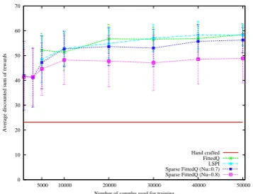
Figure 1: FittedQ policy evaluation statistics
from1.103to50.103 samples (no convergence of weights was observed with fewer samples than 1.103). The training is repeated for each of the 8 training data sets. Dictionary computed using dif-ferent number of training samples and withν=0.7 and 0.8 had a maximum of 367 and 306 elements respectively (with lower values of ν the number of features is higher than the hand-selected ver-sion). The policies learned were then tested us-ing a unigram user simulation and theDIPPER di-alogue management framework. Figures 1 and 2 show the average discounted sum of rewards of policies tested over 8×25 dialogue episodes.
5.5 Analysis of evaluation results
Our experimental results show that the dialogue policies learned using sparse SLFQ and LSPI with the two different Q-function representations per-form significantly better than the hand-coded pol-icy. Most importantly it can be observed from Figure 1 and 2 that the performance of sparse LSFQ and sparse LSPI (which uses the dictionary method for feature selection) are nearly as good as LSFQ and LSPI (which employs more numer-ous hand-selected basis functions). This shows the effectiveness of using the dictionary method for learning the representation of theQ-function from the dialogue corpora. For this specific problem the set of hand selected features seem to perform better than sparse LSPI and sparse LSFQ, but this may not be always the case. For complex dialogue management problems feature selection methods such as the one studied here will be handy since the option of manually selecting a good set of fea-tures will cease to exist.
Secondly it can be concluded that, similar to LSFQ and LSPI, the sparse LSFQ and sparse LSPI based dialogue management are also sample
0 10 20 30 40 50 60 70
5000 10000 20000 30000 40000 50000
Average discounted sum of rewards
Number of samples used for training Hand crafted
LSPI Sparse-LSPI (Nu=0.7) Sparse-LSPI (Nu=0.8)
Figure 2: LSPI policy evaluation statistics
cient and needs only few thousand samples (recall that a sample is a dialogue turn and not a dialogue episode) to learn fairly good policies, thus exhibit-ing a possibility to learn a good policy directly from very limited amount of dialogue examples. We believe this is a significant improvement when compared to the corpora requirement for dialogue management using other RL algorithms such as SARSA. However, sparse LSPI seems to result in poorer performance compared to sparse LSFQ.
One key advantage of using the dictionary method is that only mandatory basis functions are selected to be part of the dictionary. This results in fewer feature weights ensuring faster conver-gence during training. From Figure 1 it can also be observed that the performance of both LSFQ and LSPI (using hand selected features) are nearly identical. From a computational complexity point of view, LSFQ and LSPI roughly need the same number of iterations before the stopping criterion is met. However, reminding that the proposed LSFQ complexity is O(p)2 per iteration whereas LSPI complexity isO(p3)per iteration, LSFQ is computationally less intensive.
6 Discussion and Conclusion
[image:7.595.323.503.78.215.2]state-of-the-art algorithms (such as (Li et al., 2009; Hen-derson et al., 2008)). Yet the number of features is also increased. Using a sparsification algorithm, this number is reduced while policy performances are kept. In the future, more compact representa-tion of the state-acrepresenta-tion value funcrepresenta-tion will be in-vestigated such as neural networks.
Acknowledgments
The work presented here is part of an ongoing re-search for CLASSiC project (Grant No. 216594, www.classic-project.org) funded by the European Commission’s 7thFramework Programme (FP7).
References
Richard Bellman and Stuart Dreyfus. 1959. Functional approximation and dynamic programming. Math-ematical Tables and Other Aids to Computation, 13:247–251.
Richard Bellman. 1957. Dynamic Programming. Dover Publications, sixth edition.
Steven J. Bradtke and Andrew G. Barto. 1996. Lin-ear Least-Squares algorithms for temporal differ-ence learning. Machine Learning, 22(1-3):33–57.
Wieland Eckert, Esther Levin, and Roberto Pieraccini. 1997. User Modeling for Spoken Dialogue System Evaluation. InASRU’97, pages 80–87.
Yaakov Engel, Shie Mannor, and Ron Meir. 2004. The Kernel Recursive Least Squares Algorithm. IEEE Transactions on Signal Processing, 52:2275–2285.
Damien Ernst, Pierre Geurts, and Louis Wehenkel. 2005. Tree-Based Batch Mode Reinforcement Learning. Journal of Machine Learning Research, 6:503–556.
Geoffrey Gordon. 1995. Stable Function Approxima-tion in Dynamic Programming. InICML’95.
James Henderson, Oliver Lemon, and Kallirroi Georgila. 2008. Hybrid reinforcement/supervised learning of dialogue policies from fixed data sets. Computational Linguistics, vol. 34(4), pp 487-511.
Michail G. Lagoudakis and Ronald Parr. 2003. Least-squares policy iteration. Journal of Machine Learn-ing Research, 4:1107–1149.
Staffan Larsson and David R. Traum. 2000. Informa-tion state and dialogue management in the TRINDI dialogue move engine toolkit. Natural Language Engineering, vol. 6, pp 323–340.
Oliver Lemon, Kallirroi Georgila, James Henderson, and Matthew Stuttle. 2006. An ISU dialogue sys-tem exhibiting reinforcement learning of dialogue policies: generic slot-filling in the TALK in-car sys-tem. InEACL’06, Morristown, NJ, USA.
Esther Levin and Roberto Pieraccini. 1998. Us-ing markov decision process for learnUs-ing dialogue strategies. InICASSP’98.
Lihong Li, Suhrid Balakrishnan, and Jason Williams. 2009. Reinforcement Learning for Dialog Man-agement using Least-Squares Policy Iteration and Fast Feature Selection. InInterSpeech’09, Brighton (UK).
Olivier Pietquin and Thierry Dutoit. 2006. A prob-abilistic framework for dialog simulation and opti-mal strategy learning. IEEE Transactions on Audio, Speech & Language Processing, 14(2): 589-599.
Olivier Pietquin. 2005. A probabilistic descrip-tion of man-machine spoken communicadescrip-tion. In ICME’05, pages 410–413, Amsterdam (The Nether-lands), July.
Martin L. Puterman. 1994. Markov Decision Pro-cesses: Discrete Stochastic Dynamic Programming. Wiley-Interscience, April.
Jost Schatzmann, Matthew N. Stuttle, Karl Weilham-mer, and Steve Young. 2005. Effects of the user model on simulation-based learning of dialogue strategies. InASRU’05, December.
Jost Schatzmann, Karl Weilhammer, Matt Stuttle, and Steve Young. 2006. A survey of statistical user sim-ulation techniques for reinforcement-learning of dia-logue management strategies. Knowledge Engineer-ing Review, vol. 21(2), pp. 97–126.
Bernhard Scholkopf and Alexander J. Smola. 2001. Learning with Kernels: Support Vector Machines,
Regularization, Optimization, and Beyond. MIT
Press, Cambridge, MA, USA.
Satinder Singh, Michael Kearns, Diane Litman, and Marilyn Walker. 1999. Reinforcement learning for spoken dialogue systems. InNIPS’99. Springer.
Richard S. Sutton and Andrew G. Barto. 1998. Re-inforcement Learning: An Introduction (Adaptive
Computation and Machine Learning). The MIT
Press, 3rd edition, March.
Marilyn A. Walker, Diane J. Litman, Candace A. Kamm, and Alicia Abella. 1997. PARADISE: A framework for evaluating spoken dialogue agents.
InACL’97, pages 271–280, Madrid (Spain).
Jason Williams and Steve Young. 2005. Scaling up pomdps for dialogue management: the summary pomdp method. InASRU’05.
Jason D. Williams and Steve Young. 2007. Partially observable markov decision processes for spoken di-alog systems. Computer Speech and Language, vol. 21(2), pp. 393–422.
Appendix
This appendix provides pseudo code for the algo-rithms described in the paper.
Algorithm 1:Sparse LSFQ.
Initialization;
Initialize vectorθ0, choose a kernelKand a sparsification factorν;
Compute the dictionary;
D={(˜sj,a˜j)1≤j≤p}from{(sj, aj)1≤j≤N};
Define the parametrization;
Qθ(s, a) =θTφ(s, a)withφ(s, a) =
(K((s, a),(˜s1,˜a1)), . . . , K((s, a),(˜sp,a˜p)))T;
ComputeP−1;
P−1 = (PN
j=1φjφTj)−1;
fork= 1,2, . . . , M do Computeθk, see Eq. (7);
end
ˆ
π∗M(s) = argmaxa∈AQˆθM(s, a);
Algorithm 2:Sparse LSPI.
Initialization;
Initialize policyπ0, choose a kernelKand a sparsification factorν;
fork= 1,2, . . . do
Compute the dictionary;
D={(˜sj,a˜j)1≤j≤pk}from
{(sj, aj)1≤j≤N,(sj0, πk−1(sj0))1≤j≤N};
Define the parametrization;
Qθ(s, a) =θTφ(s, a)withφ(s, a) =
(K((s, a),(˜s1,a˜1)), . . . , K((s, a),(˜spk,a˜pk))) T;
Computeθk−1, see Eq. (6);
Computeπk;
πk(s) = argmaxa∈AQˆθk−1(s, a);