in Genetic Algorithms
Martin Serpell
[email protected]Department of Computer Science, University of the West of England, Bristol, BS161QY, United Kingdom
James E. Smith
[email protected]Department of Computer Science, University of the West of England, Bristol, BS161QY, United Kingdom
Abstract
The choice of mutation rate is a vital factor in the success of any genetic algorithm (GA), and for permutation representations this is compounded by the availability of several alternative mutation operators. It is now well understood that there is no one “optimal choice”; rather, the situation changes per problem instance and during evolution. This paper examines whether this choice can be left to the processes of evolution via self-adaptation, thus removing this nontrivial task from the GA user and reducing the risk of poor performance arising from (inadvertent) inappropriate decisions. Self-adaptation has been proven successful for mutation step sizes in the continuous domain, and for the probability of applying bitwise mutation to binary encodings; here we examine whether this can translate to the choice and parameterisation of mutation operators for permutation encodings.
We examine one method for adapting the choice of operator during runtime, and several different methods for adapting the rate at which the chosen operator is applied. In order to evaluate these algorithms, we have used a range of benchmark TSP prob-lems. Of course this paper is not intended to present a state of the art in TSP solvers; rather, we use this well known problem as typical of many that require a permutation encoding, where our results indicate that self-adaptation can prove beneficial. The re-sults show that GAs using appropriate methods to self-adapt their mutation operator and mutation rate find solutions of comparable or lower cost than algorithms with “static” operators, even when the latter have been extensively pretuned. Although the adaptive GAs tend to need longer to run, we show that is a price well worth paying as the time spent finding the optimal mutation operator and rate for the nonadaptive versions can be considerable. Finally, we evaluate the sensitivity of the self-adaptive methods to changes in the implementation, and to the choice of other genetic operators and population models. The results show that the methods presented are robust, in the sense that the performance benefits can be obtained in a wide range of host algorithms.
Keywords
Genetic algorithms, self-adaptation, mutation, permutation encodings.
1
Introduction
parameters has been proven successful in the continuous domain (Beyer, 2001; Schwefel, 1981) and for binary combinatorial problems (B¨ack, 1992; Glickman and Sycara, 2000; Preuss and Bartz-Beielstein, 2007; Smith and Fogarty, 1996). Removing the need for the GA user to find optimal settings for the mutation operator and/or rate saves them a considerable amount of time. It can also reduce the risk of poor performance arising from inappropriate settings when extensive operator tuning is not possible or practical, and so can improve performance over a wider range of problem instances.
Here we look at combinatorial problems with a permutation representation, where there are many possible mutation operators to choose from, each with an associated parameter. In order to exemplify this class of problems, we have taken as our benchmark well-known examples of the travelling salesman problem (TSP). Of course this paper is not intended to present a state of the art in TSP solvers; rather, we use this as typical of many that require a permutation encoding. In this paper, we investigate the self-adaptation of the mutation operator, the self-self-adaptation of the mutation rate, and the self-adaptation of the mutation operator and rate combined.
The rest of this paper proceeds as follows. Section 2 provides background on self-adaptation and on different mechanisms that have been used to achieve it. Section 3 describes our experimental setup, that is, the choice of problems, algorithmic frame-work, performance measures, and algorithms used for comparison. Section 4 describes experiments to select the best fixed mutation operator and mutation rate for our test problems; the results were then to be used as a benchmark to test self-adaptation. Sec-tion 5 describes experiments evaluating various possible mechanisms for self-adapting the mutation probability, and their robustness to changes in implementation details. Section 6 describes experiments using self-adaptation to evolve the choice of mutation operator to be applied to any particular offspring. Section 7 evaluates the effects of self-adapting both the choice of mutation operator and its probability of application. Sec-tion 8 evaluates whether or not self-adaptaSec-tion is effected by the particular GA set-up by examining other population models and choices of operator for selection and crossover. Finally, in Section 9 we draw some conclusions and suggest areas for future work.
2
Background on Self-Adaptation
Genetic algorithms (GAs) are search methods based on evolution in nature. In GAs, a solution to the search problem is encoded in a chromosome. As in nature, these chromosomes undergo recombination (crossover) and mutation to produce offspring. These offspring then replace the less fit members of the population. In this way, the GA moves toward better solutions. GAs are typically used for NP-hard problems where finding the optimal solution would take far too long to calculate, they will typically find a good solution within a reasonable time. In order to get good results using a GA, one needs good parameters such as the selection strategy, the crossover rate, the mutation rate, the mutation operator, and the replacement strategy. It is not uncommon for a large amount of time to be spent tuning these parameters in order to optimise the GA performance (Eiben et al., 2007; Meyer-Nieberg and Beyer, 2007). Often the parameters selected will only be optimal for a particular problem type or problem instance (Eiben and Smith, 2003).
had relatively less success, and there has been natural interest in the application of evo-lutionary algorithms to search this space. In particular, the use of self-adaptation, where the operator’s parameters are encoded within the individuals and subjected to evolution was established in the continuous domain within evolution strategies (Schwefel, 1981). B¨ack’s work in self-adapting the mutation rate to use for binary encodings within gener-ational GAs (B¨ack, 1992) proved the concept, and established the need for appropriate selection pressure. Smith and Fogarty (1996) examined the encoding and conditions necessary to translate this to a steady-state GA. In order to achieve the necessary selec-tion pressure, they employed a cloning mechanism. From the single offspring resulting from crossover, they derived a set of clones. The mutation rate of each clone was then modified with a certain probability before being applied. The fittest resulting solution was then returned to the population. The results showed that the number of clones that led to the shortest tour length was five, and that this tallied with previous work
in evolution strategies (where the ratio ofμtoλis typically in the range of 5–7) and
B¨ack’s implementation of truncation selection. They found that adding a self-adaptive mutation rate improved the performance of the GA and removed a nontrivial parameter from the GA. They also examined a variety of different ways of encoding the mutation parameter. In subsequent work, Stone and Smith (2002) showed that for combinatorial problems, the use of a continuous variable to encode for the mutation rate, subject to log-normal adaptation, was outperformed by a simpler scheme. In their method, the value of the gene encoding for the mutation rate had a discrete set of alleles, that is, the mutation rate came from a fixed set, and when subject to mutation was randomly reset with a small probability. This has been examined experimentally and theoretically in Smith (2001, 2003). In particular, it was shown that the way that the encoded muta-tion rate is perturbed is important—allowing the operator to work on-itself (per B¨ack, 1992)—will lead to premature convergence to suboptimal attractors. Similar results have been found in the continuous domain experimentally (e.g., Glickman and Sycara, 1999) and theoretically (Rudolph, 2001). Stephens et al. (1998) have shown in general that adding self-adaptive genes to encodings can create evolutionary advantages.
Extending beyond adapting the rate at which an operator is applied, B¨ack et al. (2000) explored self-adaptation applied to the population size, the mutation rate, and the crossover rate on a set of five test functions. They found that self-adapting all three parameters or the population size alone performed better than the equivalent standard GA. They were disappointed with the performance of self-adapting the mutation rate alone and the crossover rate alone. They concluded that one reason for the poor results of the GA with a self-adapting mutation rate alone was their chosen algorithm, and that the one used by Smith and Fogarty (1996) has been shown to perform better. This work was followed by Eiben, Schut, and de Wilde (2006), who used self-adaptation of population size and tournament size based on aggregated data from the population; they used a self-adaptive mutation rate GA as one of their benchmarks.
Others have explored evolving the whole GA to solve the TSP problem (Oltean, 2005). Although there has been work on self-adapting the choice and mechanisms of the crossover operator (Schaffer and Morishima, 1987; Spears and Anand, 1991; Smith and Fogarty, 1995, 1996), and of local search strategy (Hart et al., 2004; Krasno-gor and Gustafson, 2004; Smith, 2002, 2007b), there has to date been little attention
paid to thechoiceof mutation operator. This is perhaps because work in this area has
is changed, the whole landscape changes, which is quite different from continuous or bitwise binary operators where you have a fully connected weighted graph. An inves-tigation as to how different operators affect the fitness landscape can be seen (Julstrom, 1997; Thierens, 2005; Reeves, 1999; Schiavinotto and Stutzle, 2007).
3
Experimental Setup
A steady-state GA was used for all experiments. The parent population was set to 100, the mating population was set to 2, and there was 1 offspring. Selection was via binary tournament, the crossover probability was 0.7, and the crossover type was DPX (Friesleben and Merz, 1996; Merz and Freisleben, 1997). Replacement was via binary tournament between the offspring and the oldest parent. Each experiment was run 20 times for statistical analysis. In these experiments, the mutation rate was the probability that each gene in the chromosome will mutate and not the probability that a single mutation will occur in the chromosome. The steady-state GAs were allowed to run for up to 5,000,000 calls to the fitness function or until there was no improvement for 200,000 iterations. The results were recorded and analysed. All experiments were carried out on 27 problem instances from TSPLIB (Reinelt, 1991), and the problem instances ranged in size from 48 nodes to 657 nodes.
The mutation operators for permutation representations must ensure that the chro-mosome post mutation is a permutation of the chrochro-mosome prior to mutation. The mutation operators considered are as follows.
SWAP Swap the allele value in the locus currently being considered with that
from another randomly chosen location.
INSERT Move the allele value from the locus currently being considered to that
of another randomly chosen location.
SCRAMBLE Scramble the allele values between the locus currently being considered
and that of another randomly chosen location.
INVERSION Reverse the sequence of the allele values between the locus currently
being considered and that of another randomly chosen location.
ASSORTED Carry out a SWAP, INSERT, SCRAMBLE, or INVERSION each time a
mutation operation is required. Each operator is selected in sequence.
A detailed description of these mutation operators can be found in Eiben and Smith (2003).
There are many other types of mutation operator, such as the TRANSLOCATION mutation operator, that we have not included in this paper. We chose a limited number of operators with which to investigate self-adaptation for simplicity. However during our research it has become apparent that, as each mutation operator provides its own unique way to escape a local minima, using a larger set of mutation operators would be interesting. This may form the basis of future research.
In order to compare the results on individual TSP instances, we used one-way ANOVA testing to see if there was a significant difference between the cost of the solu-tions found using methods. Where this was indicated with more than 95% confidence, post-hoc analysis with Tamhane’s T2 test was used to determine whether pairwise differences were statistically significant. Where enough runs of the GAs for a given problem instance had terminated due to stability, we used one-way ANOVA to see whether there was a significant difference between the numbers of calls to the fitness function for the nonadaptive GA as opposed to the self-adaptive GAs. This is of sec-ondary importance when compared to which GA provides the cheapest cost for the travelling salesman, but would be used to recommend which GA to use should two or more GAs provide the cheapest solution.
In order to draw more general conclusions, a full ANOVA with the algorithm and instance as independent factors was carried out, again with post-hoc testing between algorithms. Tamhane’s T2 test is used for post-hoc analysis as it does not assume that the sets of results being compared have equal variances. However, there still remains the issue of whether the runs from different TSP instances can be normalised in a consistent manner, particularly when in some cases getting close to the optimum presents a hard bound which makes the assumption of a Gaussian distribution invalid. Thus for greater confidence, in some cases we also report results from using the nonparametric Kruskal-Wallis test. This is based on the rankings of results attained by different methods rather than their absolute values, and so is more conservative.
4
Selecting the Best Fixed Mutation Operator and Rate
An initial set of experiments was carried out to determine which mutation operator and mutation rate produce the shortest tour length within the context of our “standard” steady-state GA. The results obtained using the mutation operator and mutation rate that produced the shortest tour length were then used as base data for comparison in the further experiments.
4.1 Experimental Setup
A steady-state GA was applied 20 times for each of the five mutation operators and 13 different mutation rates (0.001, 0.005, 0.01, 0.015, 0.02, 0.025, 0.03, 0.035, 0.04, 0.045, 0.05, 0.055, and 1/length) on each of the problem instances.
4.2 Results
Using the general model statistical analysis of the best solution found per run with each of the fixed mutation rates showed that using a mutation rate of 0.005 performed
significantly better (>95% confidence) than the others.
rate 0.005, however neither of these mutation rates sat in the centre of each sweet spot, the function defining this mutation rate was not found.
A comparison was made of the performance of the four mutation operators (SWAP, INSERT, SCRAMBLE, and INVERSION), ignoring ASSORTED. This showed that for each problem instance INVERSION outperformed the other three mutation operators; see Table 5 discussed later. We then used ANOVA/Tamhane to analyse the results for all five mutation operators, factoring out the effect of instance.
• Considering all mutation rates INVERSION was significantly better (>95%
con-fidence) than both SWAP and SCRAMBLE.
• Considering a mutation rate of 0.005 both INVERSION and ASSORTED
per-formed significantly better (>95% confidence) than SWAP, INSERT, and
SCRAMBLE.
• Considering a mutation rate of 1/length showed that SWAP, INSERT,
INVERSION, and ASSORTED performed significantly better (>95% confidence)
than SCRAMBLE. It also showed that ASSORTED outperformed SWAP, INSERT, and INVERSION but not significantly.
It is likely that had more runs been made, this difference would have become sta-tistically significant. This result—that even on these well-understood problems there is a benefit to using more than one mutation operator—supports our hypothesis that it will be beneficial to adapt the operator choice. This is because changing the mu-tation operator changes the neighbourhood seen during mumu-tation, and so facilitates escape from points that are locally optimal under one mutation operator. This effect has been exploited elsewhere, for example, in variable neighbourhood search (Hansen and Mladenovi`c, 1998), Hyper-Heuristics (Cowling et al., 2001), and so-called multi-meme algorithms (e.g., Krasnogor et al., 2002; Ong et al., 2006; Smith, 2007a).
Using the Bonferroni test, the results were more clear cut. The ASSORTED mutation operator significantly outperformed all the others at the 95% confidence level.
The results from the algorithm with the ASSORTED mutation operator and a mu-tation rate of 1/length of the tour was used as the base data for future comparisons.
5
Self-Adapting the Choice of the Mutation Rate
Next we investigated self-adaptation of the mutation rate. In order to code for this, a gene was added to each chromosome to be used during mutation, which has different meanings according to the various mechanisms examined. The factors considered were the choice of algorithm that could be used, the lower and upper bounds of any sets of mutation rates, and the number of discrete mutation rates that should lie between the lower and upper bounds. Where we are comparing more than two things, we use the general model. When we compare two things, we also show analysis by instance. Thus the following experiments were run.
• Sensitivity to changing the method for self-adapting the mutation rate.
• Sliding-window or random selection of new values when using the discrete method.
• Sensitivity to changing the number of mutation rates when using the discrete
• Sensitivity to changing the length based lower and upper bounds for mutation range.
• Sensitivity to changing the number of length based mutation rates.
• Sensitivity to changing the values of the perturbation probability.
5.1 Sensitivity to Changing the Method for Self-Adapting the Mutation Rate
Three different algorithms for self-adapting the mutation rate are compared as follows:
1. Log normal
2. Uniform random
3. Discrete mutation rates
For the log normal and uniform random algorithms, the “mutation” gene is a
continuous variable in the range [0.0005,0.1], which directly encodes the
probabil-ity of each gene having mutation applied. For the discrete algorithm, this gene takes
the integer values in the range [0, n−1] which indexes a table ofn actual mutation
rates. This use of sets of discrete mutation rates has been shown to be successful (e.g., Smith, 2001; Stone and Smith, 2002; Smith, 2003). The possible mutation rates are shown in Table 7, discussed later. In each case the “mutation” genes were initialised randomly.
The ASSORTED mutation operator was used. During crossover the mutation rate was taken as the mean value of that in the two parents (mapped to the nearest value in the discrete case). After crossover, five clones were produced from the single offspring. The mutation rate gene was copied from the offspring to the five clones. Mutation was then applied to the five clones—first to the encoded mutation rate, then to the problem encoding with the (possibly new) probability.
For the uniform random and discrete mutation rates algorithms, the mutation rate was changed 10% of the time to a new value chosen uniformly at random from the appropriate available range, the other 90% of the time it remained unchanged. The discrete algorithm used 10 possible values. The new log normal mutation rate (R) was calculated using the following formula.
R =R·exp(-1/
√
d)·N(0,1) (1)
The constantd was first the number of nodes in the problem instance. This produced
very poor results, and after some experimentation the value was changed to 7, which performed only marginally better. Although self-adaptive mutation in the continuous domain has been reported to be relatively insensitive to this value, it has been shown elsewhere that for combinatorial problems the value can be significant (Stone and Smith, 2002).
Analysis of the results using both ANOVA/Tamhane and the Kruskal-Wallis test showed that with more than 95% confidence the discrete mutation rates algorithm per-formed significantly better than uniform random algorithm, which in turn perper-formed better than the log normal algorithm when compared over the 27 problem instances.
mutation rates algorithm. This was because the mutation rates had evolved to such low levels that within the time allowed by the convergence termination criterion (200,000 evaluations), mutation had a very low probability of causing the multiple changes needed to find a better solution and escape from a local optima. We reason that the difficulty lies in the way that the mutation rate can move to a higher value. For most problems, for much of the range of the mutation rate, a gene taking that value will on average cause less than one mutation. Thus the implicit self-adaptation fitness landscape will be neutral in these regions. The uniform random method will place the gene back in this region approximately half of the time, so the chances of escape become lower. Considering the mechanism used in log-normal adaptation, half of the time this will reduce the encoded mutation rate. If we consider any two different mutation rates, then because the mechanism is multiplicative, the chance of generating the step needed to move from the higher to the lower, is greater than that of generating a step from the lower to the higher, with a probability that increases with their distance. Thus, once the “fitness-neutral” region of the mutation-rate space is entered, there is downward pressure on mutation rates.
Similar results have been found for binary encoded problems and the case inves-tigated (Stone and Smith, 2002). These effects have been observed in the continuous domain: experimentally using self-adaptive log-normal adaptation by Glickman and Sycara (Glickman and Sycara, 2000) and theoretically using the 1:5 rule with multiplica-tive adaptation by Rudoloph (2001). Nevertheless, for many problems the log normal approach works extremely well in real-valued evolution strategies. Our hypothesis is
that the different nature of the mutation operators—in effect, the differentmeaningof the
rate that is evolved—means that this problem of premature convergence of mutation rates can be much worse in combinatorial problems.
In contrast, the discrete method is able to move to very different mutation rates, and the chance of moving (albeit temporarily) to a high value is greater and in fact becomes more so as the encoded rate decreases. Thus, although the ability to keep low mutation rates to fine-tune a solution is a little lower, so are the chances of premature convergence. Thus, the discrete mutation rates algorithm achieved significantly better results, although at the expense of more calls to the fitness function.
5.2 Sliding-Window or Random Selection of Discrete Mutation Rates
when Self-Adapting the Mutation Rate
In order to test this hypothesis further, two different algorithms were employed with the discrete mechanism. The first employed a sliding-window mechanism. The value of the mutation rate gene had a 0.9 chance of remaining the same, a 0.05 chance of increasing by 1, and a 0.05 chance of decreasing by 1. With this sliding-window mechanism, the mutation rate could only change to an adjacent mutation rate in the table of actual mutation rates. The second algorithm simply replaces the value in the mutation rate
gene, with a chance of 0.1, with a random integer value between 0 andn−1, wheren
is the number of discrete rates used.
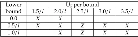
Table 1: Lower and upper bounds of the mutation rates (wherelis the number of nodes in the problem instance). X indicates the combinations examined.
Lower Upper bound
bound 1.5/ l 2.0/ l 2.5/ l 3.0/ l 3.5/ l
0.0 X X
0.5/ l X X X X X
1.0/ l X X X X
and the sliding-window algorithm can be explained as the cost involved in learning the best mutation rate. The random selection algorithm performs better than the sliding-window algorithm as it has more freedom in the changes it makes to its mutation rate. Compared to the log normal approach, we have removed the problem of the asymmetry of probabilities of moving between two values, which improved performance, but the sliding-window algorithm is still constrained to move only to adjacent mutation rates.
5.3 Sensitivity to Changing the Number of Mutation Rates
when Using the Discrete Method
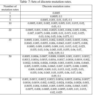
A steady-state GA was executed 20 times using seven different sets of predefined mutation rates. The sets were of sizes 1, 2, 5, 10, 22, 35, and 50. The mutation rates were not evenly distributed, but were biased toward the lower mutation rates. All mutation rates were between 0.0005 and 0.1. The actual mutation rates compared are shown in Table 7, discussed later.
Analysis using the general model both the Tamhane’s T2 test and the Kruskal-Wallis test, of the distances found for each tour, showed that the smaller sets of mutation rates performed better. The Tamhane’s T2 and Bonferroni tests both indicated that the set with five discrete mutation rates produced the shortest tour lengths, followed closely by the set with two discrete mutation rates. These tests also showed that the set with
50 discrete mutation rates performed significantly worse than the other sets (>95%
confidence).
5.4 Sensitivity to Changing the Length Based Lower and Upper Bounds
for Mutation Range
Eleven different lower and upper bounds for the mutation rates were compared, as shown in Table 1. In each experiment, 34 mutation rates were evenly distributed between the lower and upper bounds.
Analysis using the ANOVA/Tamhane showed that the mutation rates with the range from 0.5/length to 2.5/length performed better, but not significantly so at the 95% confidence level. The Kruskal-Wallis ranking also found 0.5/length to 2.5/length to be the best, followed by 0.5/length to 3.5/length, 0.5/length to 3.0/length, 1.0/length to 2.0/length, 0.5/length to 2.0/length, 0.5/length to 1.5/length, 1.0/length to 2.5/length, 1.0/length to 3.0/length, 0.0 to 1.5/length, 0.0 to 2.0/length, and 1.0/length to 3.0/length.
5.5 Sensitivity to Changing the Number of Length Based Mutation Rates
34, 40, and 50. The set with one mutation rate had a mutation rate of 1/length. All other mutation rates were evenly distributed between 0.5/length and 2.0/length.
Analysis using the ANOVA/Tamhane showed that the set containing only two mutation rates performed slightly better, but not significantly so. This is interest-ing as it agrees with the work done by Cobb and Grefenstette (1993). The dynamic switch between a low and high mutation rate (hyper-mutation) is also used in solving multi-objective problems (Abbass, 2002; Castillo and Trujillo, 2005). The set containing 20 mutation rates performed second best. The single mutation rate was significantly worse than the sets with multiple mutation rates at the 95% confidence level. Analy-sis using the Kruskal-Wallis test, which removes any bias toward the larger problem instances, showed that the set containing 20 mutation rates performed slightly better, but not significantly so. These results indicate that the number of mutation rates is not the important factor. The important factor is that there are both high and low mutation rates as this provides the opportunity for the GA to select a higher mutation rate when it is stuck in a local minima, which in turn may dislodge the GA from the local minima.
5.6 Sensitivity to Changing the Values of the Perturbation Probability
Four different probabilities were applied to changing the mutation rate. These were 0.01,
0.05, 0.1, and 0.25. The value 0.1 is the value used in all other experiments in this paper.
Analysis using the ANOVA/Tamhane showed that for the four chosen probabilities for changing the mutation rate, there was no significant difference at the 95% confidence level in the performance of the algorithm. Indeed, the algorithm has shown itself to be extremely robust to the choice of this probability of change. This is because the cloning algorithm acts as a local search within parameter space, reducing the effect of the meta-mutation rate on the effectiveness of self-adaptation.
5.7 Conclusions
These experiments showed that an algorithm that used a set of discrete mutation rates
significantly (>95% confidence) outperformed ones that used log normal and uniformly
random mutation rates. We presented a hypothesis of two contributing factors, which was supported by results showing that random selection of a new discrete mutation rate was better than the use of a sliding window. These experiments also showed that the selection of an appropriate set of discrete mutation rates was important. We found that although the best lower and upper bounds of the mutation rate were 0.5/length to 2.5/length, the algorithm would perform effectively with other lower and upper bounds of the mutation rate. The best selection of the size of the mutation rate set was found to be 20, although this was the least significant factor, again showing the robustness of this algorithm. The important factor was that there was a spread of mutation rates that would give a low mutation rate (0 or 1 bits per chromosome) up to a high mutation rate (2 or 3 bits per chromosome). Even changing the probability of mutating the mutation rate had no significant effect on this algorithm. Overall, these results showed that the discrete method is robust to a range of changes in its specification.
6
Self-Adapting the Choice of Mutation Operator
section, we examine whether it is worthwhile to self-adapt the choice of which operator to use at different stages of the search process. We then go on to look at the sensitivity to changing the rate at which the choice of mutation operator is mutated.
6.1 Self-Adapting the Choice of Operator
The algorithm used was exactly as for the discrete method with four values, except that in this case the mutation gene encoded for one of the four possible operators, and the mutation rate was as per the base data (1/length). Thus the only difference between this adaptive operator algorithm and the fixed (but cycling) operator algorithm that supplied the base data, was the means of choosing the mutation operator; so here we compared the difference between an algorithm that changed but did not learn against one that did.
When the results were compared, using a pairedt-test (results conformed to a
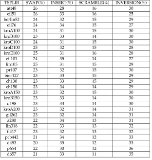
nor-mal distribution), from the 27 problem instances, 25 showed no significant difference in performance between the algorithms. The results for the other two problem instances (d657 and p654) showed that the adaptive operator algorithm performed best both times. This is an interesting result as when we compare the performance of the fixed mutation operators the INVERSION operator outperformed the ASSORTED operator for the two problem instances d657 and p654, as shown in Table 5, discussed later. This implies that the self-adaptation of the mutation operator has also found that INVER-SION is the best mutation operator to use for the problem instances d657 and p654. A comparison of the operator usage for each problem instance does indeed show that the self-adaptive GA uses the INVERSION operator more frequently for the problem instances d657 and p654 than any of the other problem instances, as shown in Table 2.
Table 2: The percentage usage of the mutation operators for each of the problem in-stances (each averaged over 20 runs) when the mutation operator is self-adapted and the mutation rate is set to 1/length.
TSPLIB SWAP(%) INSERT(%) SCRAMBLE(%) INVERSION(%)
att48 26 28 16 30
eil51 26 33 16 25
berlin52 24 32 15 29
eil76 24 34 15 27
kroA100 24 31 15 30
kroB100 23 33 14 30
kroC100 24 31 15 30
kroD100 25 32 15 28
kroE100 25 31 16 28
eil101 24 35 14 27
lin105 25 31 15 29
pr107 23 32 15 30
bier127 23 33 15 29
ch130 23 33 15 29
ch150 23 34 14 29
kroA150 23 32 15 30
kroB150 23 33 14 30
d198 23 33 14 30
kroA200 23 32 14 31
gil262 23 32 14 31
a280 22 34 13 31
lin318 22 33 13 32
fl417 23 32 13 32
pcb442 21 34 12 33
d493 20 35 12 33
p654 22 30 12 36
d657 21 33 11 35
first half of the GA search. During this time, the tour length was rapidly improved. The SWAP operator appeared later in the GA search after a short period dominated by the SCRAMBLE operator. As the GA search is initialised with random permuta-tions (i.e., scrambled data), it is possible that SWAP is the best operator for improving scrambled data. The INSERT operator is the main operator during the last 60% of the GA search, followed by INVERSION. Because these operators break fewer links, they make finer improvements to the tour length. The SCRAMBLE operator became domi-nant toward the end of the GA search for a short period of time. This is probably because the SCRAMBLE operator can rearrange small portions of the chromosome in a way that the other mutation operators could not, and this was needed to get out of local minima.
6.2 Sensitivity to Changing the Rate at which the Choice of Mutation
Operator is Mutated
Four different probabilities were applied to changing the mutation operator. These were
0.01, 0.05, 0.1, and 0.25. The value 0.1 is the value used in all other experiments in this
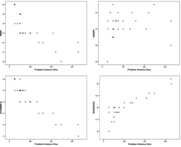
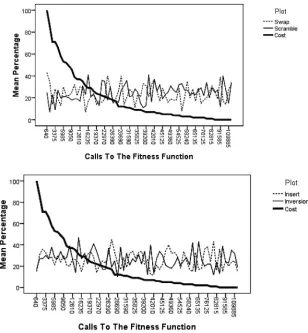
Figure 1: Mutation operator usage by problem instance size when self-adaptation is used to select the mutation operator and the mutation rate is fixed.
Analysis using the ANOVA/Tamhane showed that for the four chosen probabilities for changing the mutation operator, there was no significant difference at the 95% confidence level in the performance of the algorithm. Indeed, the algorithm has shown itself to be extremely robust to the choice of this probability of change.
6.3 Conclusions
These experiments have shown that self-adapting the choice of mutation operator per-forms at least as well as cycling through each of the four mutation operators (SWAP, INSERT, SCRAMBLE, and INVERSION). These experiments have shown that the choice of operator adapts to the given problem instance and will also change over time. The probability of changing the mutation operator has little effect on the performance of
this algorithm, no significant effect being detected when the probabilities 0.01, 0.05, 0.1,
and 0.25 were examined. This leads us to conclude that this is a robust algorithm.
7
Self-Adapting the Choice of Mutation Operator and Rate
Simultaneously
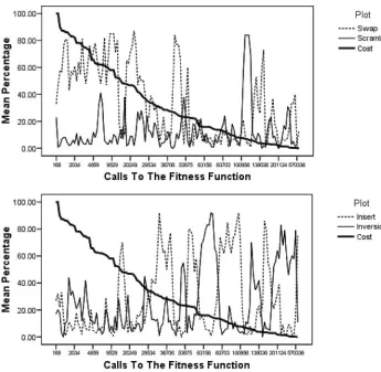
Figure 2: Mutation operator usage over time for problem instance att48, where only the mutation operator is self-adapted. The top graph shows the usage of the SWAP and SCRAMBLE operators. The bottom graph shows the usage of the INSERT and INVERSION operators. The graphs are split this way for purposes of clarity.
rate, then two of the parameters normally required to be set up by the user of the GA have been removed.
7.1 Experimental Setup
To each chromosome, a gene was added to code for the mutation operator and a gene to code for the mutation rate; see Section 3. The adaptive rate adaptive operator algorithm was run 20 times for each of the same 27 problem instances from TSPLIB (Reinelt, 1991). The results were compared against the nonadaptive base data which used the ASSORTED operator and a mutation rate of 1/length.
7.2 Results
Normalizing the results and factoring out the effect of the problem instance revealed that the tour lengths obtained with the self-adaptive GA are significantly shorter than
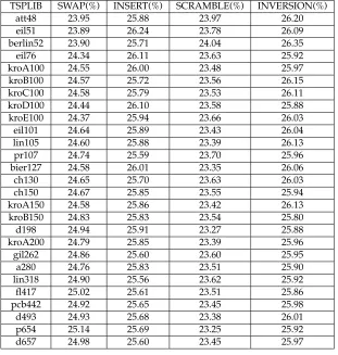
Table 3: The percentage usage of the mutation operators for each of the problem in-stances (each averaged over 20 runs) when both the mutation operator and rate are self-adapted.
TSPLIB SWAP(%) INSERT(%) SCRAMBLE(%) INVERSION(%)
att48 23.95 25.88 23.97 26.20
eil51 23.89 26.24 23.78 26.09
berlin52 23.90 25.71 24.04 26.35
eil76 24.34 26.11 23.63 25.92
kroA100 24.55 26.00 23.48 25.97
kroB100 24.57 25.72 23.56 26.15
kroC100 24.58 25.79 23.53 26.11
kroD100 24.44 26.10 23.58 25.88
kroE100 24.37 25.94 23.66 26.03
eil101 24.64 25.89 23.43 26.04
lin105 24.60 25.88 23.39 26.13
pr107 24.74 25.59 23.70 25.96
bier127 24.58 26.01 23.35 26.06
ch130 24.65 25.70 23.63 26.03
ch150 24.67 25.85 23.55 25.94
kroA150 24.58 25.86 23.42 26.13
kroB150 24.83 25.83 23.54 25.80
d198 24.94 25.91 23.27 25.88
kroA200 24.79 25.85 23.39 25.96
gil262 24.86 25.60 23.60 25.95
a280 24.76 25.83 23.51 25.90
lin318 24.90 25.56 23.62 25.92
fl417 25.02 25.61 23.51 25.86
pcb442 24.92 25.65 23.45 25.98
d493 24.93 25.68 23.38 26.01
p654 25.14 25.69 23.25 25.92
d657 24.98 25.60 23.45 25.97
The usage of mutation operators is given in Table 3 for each of the problem instances. This shows that self-adaptation of the mutation operator plays a lesser role when the mutation rate is being self-adapted. Effectively, the self-adaptation of the mutation rate all but shuts down the self-adaptation of the mutation operator. The percentage usage of the operators remained extremely constant throughout the experiment. However, the mutation of the operator still plays an important part in finding the shortest path. If we look at Table 5, discussed later, we can see that self-adapting the choice of mutation operator alone found the best solution in four of the 27 problem instances. For seven other problem instances, self-adapting the choice of mutation operator alone performed better than self-adapting the choice mutation rate alone, but combining both types of self-adaptation performed even better, showing that there is a synergy to be exploited. During the experiment, for problem instance a280, the mutation rate fluctuated between 0.0025 and 0.0058. This is equivalent to an average of 0.7 to 1.624 bit mutations per clone per iteration.
Figure 3: Mutation operator usage over time for problem instance att48, where both the mutation operator and mutation rate are self-adapted.
Table 4: Comparison of the results obtained using a self-adaptive GA with the known optimal results. The published optimal solution comes from the TSPLIB website. The calculated optimal solution is produced using our costing function (which is imple-mented with lower precision than that of TSPLIB and also treats all TSPLIB data as being in EUC 2D format) on the TSPLIB published tour, where tours have been published.
Published Calculated Self-adaptive GA Percentage
TSPLIB Optimal Optimal Shortest Longest Mean SD Difference
att48 10,628 33,523 33,723 34,830 34,262 304.74 0.591
eil51 426 429 429 447 439 5.05 0.001
berlin52 7,542 7,544 7,544 8,244 7,871 206.62 0.001
eil76 538 557 583 571 570 8.72 4.661
kroA100 21,282 21,285 21,480 23,506 22,423 530.54 0.911
kroB100 22,141 22,381 24,720 23,342 623.79 1.082
kroC100 20,749 20,750 20,852 23,055 21,975 628.83 0.491
kroD100 21,294 21,294 21,564 23,397 22,560 551.78 1.261
kroE100 22,068 22,357 24,356 23,083 552.93 1.302
eil101 629 624 657 686 671 8.43 5.281
lin105 14,379 14,382 14,460 15,770 15,137 368.99 0.541
pr107 44,303 44,911 49,419 46,756 1,303.84 1.372
bier127 118,282 122,709 130,695 125,073 2,067.61 3.742
ch130 6,110 6,110 6,292 6,768 6,507 147.94 2.971
ch150 6,528 6,532 6,803 7,247 7,025 131.04 4.141
kroA150 26,524 27,338 29,159 28,286 526.14 3.062
kroB150 26,130 27,076 28,723 28,060 445.88 3.622
d198 15,780 16,137 16,750 16,409 183.37 2.262
kroA200 29,368 30,719 32,790 31,682 609.00 4.602
gil262 2,378 2,504 2,694 2,591 54.92 5.292
a280 2,579 2,586 2,772 2,961 2,859 51.81 7.191
lin318 42,029 44,394 46,471 45,681 589.15 5.622
fl417 11,861 12,050 13,796 12,816 418.10 1.592
pcb442 50,778 50,783 55,303 59,106 56,864 825.72 8.901
d493 35,002 37,695 39,487 38,312 557.84 7.692
p654 34,643 38,482 43,244 40,668 1,421.73 11.082
d657 48,912 57,967 60,982 59,023 1,005.78 18.512 1The percentage difference is the percentage difference between the self-adaptive GAs shortest tour and the distance of the tour calculated using our cost function.
2The percentage difference is the percentage difference between the self-adaptive GAs shortest tour and the distance published on the TSPLIB website.
Our results show that self-adapting the mutation rate is computationally cheaper than adapting the mutation operator; however, the best result is achieved by self-adapting both.
7.3 Full Comparison of Results
of the self-adaptive GA on the larger problem instances was most likely due to the limitation placed on the number of calls to the fitness function.
Table 5 contains a comparison of the results obtained using nonadaptive GAs that used the five different mutation operators, SWAP, INSERT, SCRAMBLE, INVERSION, and ASSORTED against three self-adaptive GAs, one that only adapted the mutation operator, one that only adapted the mutation rate, and one that adapted both the mutation rate and mutation operator.
In each case, the best results were found using a self-adaptive algorithm. Out of the 27 problem instances, six (berlin52, d198, d657, eil76, kroA200, and kroB100) had the shortest tour lengths found when using the self-adaptive GA that adapted the mutation operator only and eight problem instances (att48, ch130, ch150, eil76, kroB150, kroC100, p654, and pcb442) had the shortest tour lengths found when using the self-adaptive GA that adapted the mutation rate only. The remaining 14 problem instances (a280, bier127, d493, eil51, eil101, fl417, gil262, kroA100, kroA150, kroD100, kroE100, lin105, lin318, and pr107) had the shortest tour lengths found when using the self-adaptive GA that adapted both the mutation rate and mutation operator. Please note that the problem instance eil76 was solved equally well by two of the self-adaptive GAs. In all cases the self-adaptive GAs were still searching for better solutions when they were terminated due to the number of fitness calls reaching a predefined limit (5,000,000).
Comparing the difference in the mean tour lengths between the best performing nonadaptive GA (mutation rate of 1/length and mutation operator is ASSORTED) and the best performing self-adaptive GA (self-adapts both the mutation rate and mutation operator) for each of the 27 problem instances showed that in each case the self-adaptive GA produced a shorter mean tour. On average, the best self-adaptive GA produced a tour length 1.8% shorter than the best nonadaptive GA.
7.4 Comparison Against a State of the Art TSP Solver
As previously stated, this paper is not intended to present the state of the art in TSP solvers. Its purpose is to examine the effect of self-adaptation of the mutation rate and mutation operator on problems with a permutation representation. We did, however, compare its performance against a state of the art TSP solver. Against the Concorde TSP Solver (Applegate et al., 1996) our self-adapting GAs took much longer to find a solution. For example, to find a solution for the problem instance KroA100, one of our GAs took 15 s compared to 1 s for the Concorde TSP Solver and required 1,000,000 calls to the fitness function.
8
Examining Different GA Setups
In order to examine whether the improved results obtained were an artifact of the par-ticular GA environment used, different GA setups were compared using self-adapting steady-state GAs and nonadapting steady-state GAs. Experiments were run that com-pared the two types of GA with the following different GA parameters.
• Different crossover operators (DPX and PMX)
• Different replacement strategies (replacing the oldest and replacing the oldest by
Table 6: Different pool size configurations.
Configuration Parent pool Mating pool Offspring pool
1 100 2 1
2 100 10 5
3 100 20 10
4 100 50 25
5 100 100 100
6 200 200 200
Table 7: Sets of discrete mutation rates.
Number of Discrete mutation rates
mutation rates
1 0.0005
2 0.0005, 0.1
5 0.0005, 0.001, 0.01, 0.05, 0.1
10 0.0005, 0.001, 0.002, 0.003, 0.005, 0.01, 0.015, 0.02, 0.05, 0.1
22 0.0005, 0.001, 0.002, 0.0025, 0.003, 0.004, 0.005, 0.006, 0.007, 0.0075, 0.008, 0.009, 0.01, 0.015, 0.02, 0.025,
0.03, 0.04, 0.05, 0.06, 0.075, 0.1
35 0.0005, 0.001, 0.0015, 0.002, 0.0025, 0.003, 0.0035, 0.004, 0.0045, 0.005, 0.0055, 0.006, 0.0065, 0.007, 0.0075, 0.008,
0.0085, 0.009, 0.0095, 0.009, 0.01, 0.015, 0.02, 0.025, 0.035, 0.03, 0.04, 0.045, 0.05, 0.055, 0.06, 0.07,
0.08, 0.09, 0.1
50 0.0005, 0.0006, 0.0007, 0.0008, 0.0009, 0.001, 0.0011, 0.0012, 0.0013, 0.0014, 0.0015, 0.0016, 0.0017, 0.0018, 0.0019, 0.002, 0.0022, 0.0024, 0.0026, 0.0028, 0.003, 0.0035, 0.004, 0.0045,
0.005, 0.0055, 0.006, 0.0065, 0.007, 0.0075, 0.008, 0.0085, 0.009, 0.0095, 0.009, 0.01, 0.015, 0.02, 0.025, 0.03,
0.035, 0.04, 0.045, 0.05, 0.055, 0.06, 0.07, 0.08, 0.09, 0.1
34 0.001, 0.0011, 0.0012, 0.0013, 0.0014, 0.0015, 0.0016, 0.0017, 0.0018, 0.0019, 0.002, 0.0022, 0.0024, 0.0026, 0.0028, 0.003,
0.0035, 0.004, 0.0045, 0.005, 0.0055, 0.006, 0.0065, 0.007, 0.0075, 0.008, 0.0085, 0.009, 0.0095, 0.009, 0.01, 0.015,
0.02, 0.025
• Different pool sizes (see Table 6)
• Different selection strategies (tournament, fitness proportionate, and truncation)
8.1 Results
Analysis using ANOVA/Tamhane showed that changing the GA setup made no dif-ference to the comparative performance of the self-adaptive GAs and the nonadapting GAs. As before, the mean tour distances tended to be shorter when self-adapting GAs were used; however, this difference was not statistically significant at the 95% confi-dence level.
[image:20.504.99.410.187.506.2]9
Conclusions and Suggested Areas for Future Work
All self-adaptive GAs provided comparable, or better results to the best choice of the nonadaptive GA. In Section 7.2, we showed that comparing the mean tour lengths in a similar way to Oltean (2005) showed that the best self-adaptive GA found solutions that were a little over 1.8% shorter than that of the best nonadaptive GA. The results of the full ANOVA, where we can factor out the effects of the instance in order to draw more general conclusions, show that the results obtained with GAs that self-adapted the mu-tation operator as well as the mumu-tation rate are shorter than for those that self-adapt the mutation rate or operator type only, but not significantly so, at the 95% confidence level. The algorithms that self-adapted their mutation rates required two to three times as many calls to the fitness function, depending on the problem size, compared to those using fixed rates found by prior experimental tuning. This overhead can be explained as the time required to find their optimal mutation rate. It was seen that the mutation rate can more than double when required.
When compared against the GA using the mutation rate set to 1/length and the fixed mutation operators (SWAP, INSERT, SCRAMBLE, and INVERSION), the GA that self-adapted the choice of mutation operator always produced a shorter tour length. In the case of the mutation operators (SWAP, INSERT, and SCRAMBLE) this was significant at the 95% confidence level. The benefit of self-adapting the choice of mutation operator was less clear when compared against the GA using the mutation rate set to 1/length and the fixed mutation operator (ASSORTED), but this was probably due to the fact that our nonadaptive GA cycles through the four mutation operators. This has given it a better chance of escaping any local minima than a similar GA using a single mutation operator. This was shown in Section 4 and in Table 5. This was particularly apparent when the mutation rate as well as the mutation operator was self-adapted.
The results imply that self-adaptation of the mutation rate takes precedence over the self-adaptation of the mutation operator. Since it is possible to compose any of the more complex operators by combinations of INVERT, it may simply be easier to search the landscape by adapting the mutation rate to find a way out of any local minima than by adapting the mutation operator.
Finally we noted that self-adaptation of the mutation rate and mutation operator brought about benefits irrespective of the settings of the other, nonmutation, GA param-eters. We have used the TSP as a means to investigate self-adaptation of the mutation rate and mutation operator, but we believe that our conclusions apply equally to all per-mutation problems, although further research may be carried out to prove this. We did not consider self-adaptive mutation strategies where there was no crossover operator. We believe that this may make an interesting future study. Likewise the self-adaptation of permutation crossover operators has not been considered in this paper, but this too would be interesting future research.
While carrying out the experiments in this paper, it was noted that the choice of mutation operator used changed as the GA hunted for a solution. It would be interesting to see how the choice of mutation operator and rate changed with the features in the landscape of the search space.
References
Applegate, D. L., Bixby, R. E., Chv´atal, V., and Cook, W. (1996). Concorde TSP solver: http:// www.tsp.gatech.edu/concorde.html.
B¨ack, T. (1992). Self adaptation in genetic algorithms. In F. Varela and P. Bourgine (Eds.),Toward a Practice of Autonomous Systems: Proceedings of the 1st European Conference on Artificial Life, pp. 263–271.
B¨ack, T., Eiben, A. E., and van der Vaart, N. A. L. (2000). An empirical study on GAs without parameters. In M. Schoenauer, K. Deb, G. Rudolph, X. Yao, E. Lutton, J. J. Merelo, and H.-P. Schwefel (Eds.),Proceedings of the 6th Conference on Parallel Problem Solving from Nature, Vol. 1917 of LNCS, pp. 315–324.
Beyer, H.-G. (2001).The theory of evolution strategies. Berlin: Springer.
Castillo, O., and Trujillo, L. (2005). Multiple objective optimization genetic algorithms for path planning in autonomous mobile robots. International Journal of Computers, Systems and Signals, 6(1), 48–63.
Cobb, H., and Grefenstette, J. (1993). Genetic algorithms for tracking changing environments. In S. Forrest (Ed.), Proceedings of the 5th International Conference on Genetic Algorithms, pp. 523–530.
Cowling, P., Kendall, G., and Soubeiga, E. (2001). A hyperheuristic approach to scheduling a sales summit.Lecture Notes in Computer Science, 2079:176–195.
Eiben, A., Michalewicz, Z., Schoenauer, M., and Smith, J. (2007). Parameter control in evolution-ary algorithms. In F. G. Lobo, C. F. Lima, and Z. Michalewicz (Eds.), Parameter Setting in Evolutionary Algorithms, Vol. 54 ofStudies in Computational Intelligence(pp. 19–46). Berlin: Springer Verlag.
Eiben, A. E., Schut, M. C., and de Wilde, A. R. (2006). Is self-adaptation of selection pressure and population size possible? A case study. In T. P. Runarsson et al. (Eds.)Proceedings of the 9th Annual Conference on Parallel Problem Solving from Nature, Vol. 4193 of LNCS, pp. 900–909.
Eiben, A., and Smith, J. (2003).Introduction to evolutionary computation. Berlin: Springer.
Friesleben, B., and Merz, P. (1996). A genetic local search algorithm for solving the symmetric and assymetric travelling salesman problem. InICEC-96, pp. 616–621.
Glickman, M., and Sycara, K. (1999). Comparing mechanisms for evolving evolvability. In A. Wu (Ed.),Proceedings of the 1999 Genetic and Evolutionary Computation Conference Workshop Program.
Glickman, M., and Sycara, K. (2000). Reasons for premature convergence of self-adaptating mutation rates. In2000 Congress on Evolutionary Computation (CEC’2000), pp. 62–69.
Hansen, P., and Mladenovi`c, N. (1998). An introduction to variable neighborhood search. In S. Voß, S. Martello, I. Osman, and C. Roucairol (Eds.), Meta-Heuristics: Advances and Trends in Local Search Paradigms for Optimization. Proceedings of MIC 97 Conference. Dordrecht, The Netherlands: Kluwer Academic Publishers.
Hart, W., Krasnogor, N., and Smith, J. (2004). Editorial introduction, special issue on memetic algorithms.Evolutionary Computation, 12(3):v–vi.
Julstrom, B. (1997). Adaptive operator probabilities in a genetic algorithm that applies three operators. InProceedings of the 1997 ACM Symposium on Applied Computing, pp. 233–238.
Krasnogor, N., and Gustafson, S. (2004). A study on the use of “self-generation” in memetic algorithms.Natural Computing, 3(1):53–76.
Merz, P., and Freisleben, B. (1997). Genetic local search for the TSP: New results. In IEEE Conference on Evolutionary Computation, pp. 159–164.
Meyer-Nieberg, S., and Beyer, H.-G. (2007). Self adaptation in evolutionary algorithms. In F. G. Lobo, C. F. Lima, and Z. Michalewicz (Eds.),Parameter Setting in Evolutionary Algorithms, pp. 47–76. Berlin: Springer.
Oltean, M. (2005). Evolving evolutionary algorithms using linear genetic programming.
Evolutionary Computation, 13(3):387–410.
Ong, Y., Lim, M., Zhu, N., and Wong, K. (2006). Classification of adaptive memetic algorithms: A comparative study.IEEE Transactions on Systems, Man and Cybernetics Part B, 36(1):141–152.
Preuss, M., and Bartz-Beielstein, T. (2007). Sequential parameter optimisation applied to self-adaptation for binary-coded evolutionary algorithms. In F. G. Lobo, C. F. Lima, and Z. Michalewicz (Eds.), Parameter Setting in Evolutionary Algorithms, pages 91–120. Berlin: Springer.
Reeves, C. (1999). Landscapes, operators and heuristic search. Annals of Operations Research, 86:473–490.
Reinelt, G. (1991). Tsplib: http://www.iwr.uni-heidelberg.de/groups/comopt/software/ tsplib95/.
Rudolph, G. (2001). Self-adaptive mutations may lead to premature convergence. IEEE Transactions on Evolutionary Computation, 5:410–414.
Schaffer, J., and Morishima, A. (1987). An adaptive crossover distribution mechanism for genetic algorithms. In J. Grefenstette (Ed.),Proceedings of the 2nd International Conference on Genetic Algorithms and Their Applications, pp. 36–40.
Schiavinotto, T., and Stutzle, T. (2007). A review of metrics on permutations for search landscape analysis.Computers and Operations Research, 34(10):3143–3153.
Schwefel, H.-P. (1981).Numerical optimization of computer models. New York: Wiley.
Smith, J. (2001). Modelling GAs with self-adaptive mutation rates. In L. Spector, E. Goodman, A. Wu, W. Langdon, H.-M. Voigt, M. Gen, S. Sen, M. Dorigo, S. Pezeshk, M. Garzon, and E. Burke (Eds.), Proceedings of the Genetic and Evolutionary Computation Conference (GECCO-2001), pp. 599–606.
Smith, J. (2002). On appropriate adaptation levels for the learning of gene linkage.Journal of Genetic Programming and Evolvable Machines, 3(2):129–155.
Smith, J. (2003). Parameter perturbation mechanisms in binary coded GAs with self-adaptive mutation. In K. De Jong, R. Poli, and J. Rowe (Eds.),Foundations of Genetic Algorithms 7, pages 329–346. Morgan Kauffman.
Smith, J. (2007a). Co-evolving memetic algorithms: A review and progress report. IEEE Transactions in Systems, Man and Cybernetics, Part B, 37(1):6–17.
Smith, J. (2007b). On replacement strategies in steady state evolutionary algorithms.Evolutionary Computation, 15(1):29–59.
Smith, J., and Fogarty, T. (1995). An adaptive poly-parental recombination strategy. In T. Fogarty (Ed.),Evolutionary Computing 2(pp. 48–61). Berlin: Springer.
Spears, W., and Anand, V. (1991). A study of crossover operators in genetic programming. In Pro-ceedings of the 6th International Symposium on Methodologies for Intelligent Systems, pp. 409–418.
Stephens, C. R., Garcia Olmedo, I., Moro Vargas, J., and Waelbroeck, H. (1998). Artificial Life, 4:183–201.
Stone, C., and Smith, J. (2002). Strategy parameter variety in self-adaption. In W. Langdon, E. Cant ´u-Paz, K. Mathias, R. Roy, D. Davis, R. Poli, K. Balakrishnan, V. Honavar, G. Rudolph, J. Wegener, L. Bull, M. Potter, A. Schultz, J. Miller, E. Burke, and N. Jonoska (Eds.),Proceedings of the Genetic and Evolutionary Computation Conference (GECCO-2002), pp. 586–593.
Thierens, D. (2005). An adaptive pursuit strategy for allocating operator probabilities. In