Modelling Sequential Text with an Adaptive Topic Model

Modelling Sequential Text with an Adaptive Topic Model

Lan Du∗

Department of Computing Macquarie University

Sydney, Australia [email protected]

Wray Buntine∗ Canberra Research Lab National ICT Australia

Canberra, Australia [email protected]

Huidong Jin∗

CSIRO Mathematics, Informatics and Statistics,

Canberra, Australia [email protected]

Abstract

Topic models are increasingly being used for text analysis tasks, often times replacing ear-lier semantic techniques such as latent seman-tic analysis. In this paper, we develop a novel adaptive topic model with the ability to adapt topics from both the previous segment and the parent document. For this proposed model, a Gibbs sampler is developed for doing poste-rior inference. Experimental results show that with topic adaptation, our model significantly improves over existing approaches in terms of perplexity, and is able to uncover clear se-quential structure on, for example, Herman Melville’s book “Moby Dick”.

1 Introduction

Natural language text usually consists of topically structured and coherent components, such as groups of sentences that form paragraphs and groups of paragraphs that form sections. Topical coherence in documents facilitates readers’ comprehension, and reflects the author’s intended structure. Capturing this structural topical dependency should lead to im-proved topic modelling. It also seems reasonable to propose that text analysis tasks that involve the structure of a document, for instance, summarisation and segmentation, should also be improved by topic models that better model that structure.

Recently, topic models are increasingly being used for text analysis tasks such as

summarisa-∗

This work was partially done when Du was at College of Engineering & Computer Science, the Australian National Uni-versity when working together with Buntine and Jin there.

tion (Arora and Ravindran, 2008) and segmenta-tion (Misra et al., 2011; Eisenstein and Barzilay, 2008), often times replacing earlier semantic tech-niques such as latent semantic analysis (Deerwester et al., 1990). Topic models can be improved by bet-ter modelling the semantic aspects of text, for in-stance integrating collocations into the model (John-son, 2010; Hardisty et al., 2010) or encouraging top-ics to be more semantically coherent (Newman et al., 2011) based on lexical coherence models (New-man et al., 2010), modelling the structural aspects of documents, for instance modelling a document as a set of segments (Du et al., 2010; Wang et al., 2011; Chen et al., 2009), or improving the under-lying statistical methods (Teh et al., 2006; Wallach et al., 2009). Topic models, like statistical parsing methods, are using more sophisticated latent vari-able methods in order to model different aspects of these problems.

In this paper, we are interested in developing a new topic model which can take into account the structural topic dependency by following the higher level document subject structure, but we hope to re-tain the general flavour of topic models, where com-ponents (e.g., sentences) can be a mixture of topics. Thus we need to depart from the earlier HMM style models, see, e.g., (Blei and Moreno, 2001; Gruber et al., 2007). Inspired by the idea that documents usually exhibits internal structure (e.g., (Wang et al., 2011)), in which semantically related units are clus-tered together to form semantically structural seg-ments, we treat documents as sequences of segments (e.g., sentences, paragraphs, sections, or chapters). In this way, we can model the topic correlation

~ µ

~

ν1 ~ν2 ~ν3 ~ν4

~ µ

~ν1 ~ν2 ~ν3 ~ν4

~ µ

~

ν1 ~ν2 ~ν3 ~ν4

(H) (S)

(M)

~ µ

~ν1 ~ν2 ~ν3 ~ν4

(B)

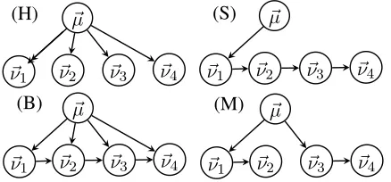
Figure 1: Different structural relationships for topics of sections in a 4-part document, hierarchical (H), sequen-tial (S), both (B) or mixed (M).

tween the segments in a “bag of segments” fashion,

i.e., beyond the “bag of words” assumption, and re-veal how topics evolve among segments.

Indeed, we were impressed by the improvement in perplexity obtained by thesegmented topic model

(STM) (Du et al., 2010), so we considered the prob-lem of whether one can add sequence information into a structured topic model as well. Figure 1 illus-trates the type of structural information being con-sidered, where the vectors are some representation of the content. STM is represented by the hierar-chical model. A strictly sequential model would seem unrealistic for some documents, for instance books. A topic model using the strictly sequential model was developed (Du et al., 2012) but it report-edly performs halfway between STM and LDA. In this paper, we develop an adaptive topic model to go beyond a strictly sequential model while allow some hierarchical influence. There are two possible hybrids, one called “mixed” has distinct breaks in the sequence, while the other called “both” overlays both sequence and hierarchy and there could be rel-ative strengths associated with the arrows. We em-ploy the “both” hybrid but use the relative strengths to adaptively allow it to approximate the “mixed” hybrid.

Research in Machine Learning and Natural Lan-guage Processing has attempted to model various topical dependencies. Some work considers struc-ture within the sentence level by mixing hidden Markov models (HMMs) and topics on a word by word basis: the aspect HMM (Blei and Moreno, 2001) and the HMM-LDA model (Griffiths et al., 2005) that models both short-range syntactic depen-dencies and longer semantic dependepen-dencies. These

models operate at a finer level than we are consider-ing at a segment (like paragraph or section) level. To make a tool like the HMM work at higher levels, one needs to make stronger assumptions, for instance as-signing each sentence a single topic and then topic specific word models can be used: the hidden topic Markov model (Gruber et al., 2007) that models the transitional topic structure; a global model based on the generalised Mallows model (Chen et al., 2009), and a HMM based content model (Barzilay and Lee, 2004). Researchers have also considered time-series of topics: various kinds of dynamic topic models, following early work of (Blei and Lafferty, 2006), represent a collection as a sequence of sub-collections in epochs. Here, one is modelling the collections over broad epochs, not the structure of a single document that our model considers.

This paper is organised as follows. We first present background theory in Section 2. Then the new model is presented in Section 3, followed by Gibbs sampling theory and algorithm in Sections 4 and 5 respectively. Experiments are reported in Sec-tion 6 with a conclusion in SecSec-tion 7.

2 Background

The basic topic model is first presented in Sec-tion 2.1, as a point of departure. In seeking to de-velop a general sequential topic model, we hope to go beyond a strictly sequential model and allow some hierarchical influence. This, however, presents two challenges: modelling and statistical inference. Hierarchical inference (and thus sequential infer-ence) over probability vectors can be handled us-ing the theory of hierarchical Poisson-Dirichlet pro-cesses (PDPs). This is presented in Section 2.2.

2.1 The LDA model

The benchmark model for topic modelling is latent Dirichlet allocation (LDA) (Blei et al., 2003), a la-tent variable model of documents. Documents are indexed byi, and words w~ are observed data. The latent variables are ~µi (the topic distribution for a

document) and~z(thetopic assignmentsfor observed words), and the model parameter ofφ~k’s (word

Ta-ble 1. The generative model is as follows:

~

φk∼DirichletW(~γ) ∀k

~

µi∼DirichletK(α~) ∀i

zi,l∼DiscreteK(~µi) ∀i, l

wi,l∼DiscreteK

~ φzi,l

∀i, l .

DirichletK(·)is aK-dimensional Dirichlet

distribu-tion. The hyper-parameter~γ is a Dirichlet prior on

word distributions(i.e., a Dirichlet smoothing on the multinomial parameterφ~k(Blei et al., 2003)) and the

Dirichlet priorα~ on topic distributions.

2.2 Hierarchical PDPs

A discrete probability vector ~µof finite dimension

K is sampled from some distribution Fτ(~µ0) with

a parameter set, say τ, and is also dependent on a parent probability vector~µ0 also of finite

dimen-sion K. Then a sample of size N is taken ac-cording to the probability vector ~µ, represented as

~

z ∈ {1, ..., K}N_{. This data is collected into counts}

~

n= (n1, ..., nK)wherenk is the number of data in

~

z with valuekandP

knk = N. This situation is

represented as follows:

~

µ ∼ Fτ(~µ0); z~i ∼ DiscreteK(~µ) fori= 1, ..., N .

Commonly in topic modelling, the Dirichlet distri-bution is used for discrete probability vectors. In this case Fτ(~µ0) ≡ DirichletK(b~µ0), τ ≡ (K, b)

where b is the concentration parameter. Bayesian analysis yields a marginalised likelihood, after inte-grating out~µ, of

p ~zτ, ~µ₀,Dirichlet

= Beta(~n+b~µ0)

Beta(b~µ0)

, (1)

where Beta(·)is the vector valued function normal-ising the Dirichlet distribution. A problem here is thatp(~z|b, ~µ0)is an intractable function of~µ0.

Dirichlet processes and Poisson-Dirichlet pro-cesses alleviate this problem by using an auxiliary variable trick (Robert and Casella, 2004). That is, we introduce an auxiliary variableover which we also sample but do not need to record. The auxiliary variable is thetable count1which is atkfor eachnk

1

Based on the Chinese Restaurant analogy (Teh et al., 2006), each table has a dish, a data value, while data, the customer, is assigned to tables, and multiple tables can serve the same dish.

and it represents the number of “tables” over which thenk“customers” are spread out. Thus the

follow-ing constraints hold:

0≤tk≤nk and tk= 0iffnk= 0. (2)

When the distribution over probability vectors fol-lows a Poisson-Dirichlet process which has two pa-rametersτ ≡ (a, b) and the parent distribution~µ0,

then Fτ(~µ0) ≡ PDP(a, b, ~µ0). Here a is the dis-count parameter,btheconcentration parameterand

~

µ0the base measure. In this case Bayesian analysis

yields an augmented marginalised likelihood (Bun-tine and Hutter, 2012), after integrating out~µ, of

p ~z, ~tτ, ~µ₀,PDP

= (b|a)T (b)N

Y

k

Snk tk,a(µ0,k)

tk ₍₃₎

whereT = P

ktk, (x|y)N = QN−1

n=0(x+ny)

de-notes the Pochhammer symbol,(x)N = (x|1)N, and

S_M,aN is a generalized Stirling number that is readily tabulated (Buntine and Hutter, 2012).

There are two fundamental things to notice about Equation (3). Positively, the term in ~µ0 takes the

form of a multinomial likelihood, so we can prop-agate it up and perform inference on ~µ0

unen-cumbered by the functional mess of Equation (1). Thus Poisson-Dirichlet processes allow one to do Bayesian reasoning on hierarchies of probability vectors (Teh, 2006; Teh et al., 2006). Negatively, however, one needs to sample the auxiliary vari-ables~tleading to some problems: The range oftk,

{0, ..., nk}, is broad. Also, contributions from

in-dividual datazi have been lost so the mixing of the

MCMC can sometimes be slow. We confirmed these problems on our first implementation of the Adap-tive Topic Model presented next in Section 3.

A further improvement on PDP sampling is achieved in (Chen et al., 2011), where another aux-iliary variable is introduced, a so-called table in-dicator, that for each datum zi indicates whether

it is the “head of its table” (recall the nk data are

spread over tk tables, each table has one and only

one “head”). Let ri = 1if zi is the “head of its

table,” and zero otherwise. According to this “ta-ble” logic, the number of tables fornk must be the

number of data zi that are also head of table, so

tk = PNi=11zi=k1ri=1. Moreover, given this

automatically satisfied. Finally, withtk tables then

there must be exactlytk heads of table, and we are

indifferent about which data are heads of table, thus

p ~z, ~rτ, ~µ₀,PDP

=p ~z, ~tτ, ~µ₀,PDP Y

k

nk

tk

−1

.

(4) When using this marginalised likelihood in a Gibbs sampler, thezithemselves are usually latent so also

sampled, and we develop a blocked Gibbs sampler for(zi, ri). Since~ronly appears indirectly through

the table counts~t, one does not need to store the~r, instead just resamples anriwhen needed according

to the proportiontw/nwwherezi =w.

3 The proposed Adaptive Topic Model In this section an adaptive topic model (AdaTM) is developed, a fully structured topic model, by using a PDP to simultaneously model the hierarchical and the sequential topic structures. Documents are as-sumed to be broken into a sequence of segments. Topic distributions are used to mimic the subjects of documents and subtopics of their segments. The no-tations and terminologies used in the following sec-tions are given in Table 1.

In AdaTM, the two topic structures are captured by drawing topic distributions from the PDPs with two base distributions as follows. The document topic distribution~µi and thejth segment topic

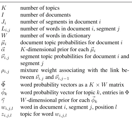
dis-Table 1: List of notation for AdaTM

K number of topics

I number of documents

Ji number of segments in documenti Li,j number of words in documenti, segmentj W number of words in dictionary

~

µi document topic probabilities for documenti ~

α K-dimensional prior for each~µi ~

νi,j segment topic probabilities for documentiand

segmentj

ρi,j mixture weight associating with the link be-tween~νi.jand~νi,j−1

~

Φ word probability vectors as aK×W matrix

~

φk word probability vector for topick, entries inΦ

~γ W-dimensional prior for eachφk~

wi,j,l word in documenti, segmentj, positionl zi,j,l topic for wordwi,j,l

w

L

z

I

K α

μ

ν

γ φ

1 ν2

1 w

L

z

2 。。。

νJ

w

L

z

J 。。。 λ

Figure 2: The adaptive topic model:~µ is the document topic distribution,~ν1, ~ν2, . . . , ~νJ are the segment topic distributions, and~ρis a set of the mixture weights.

tribution ~νi,j are linearly combined to give a base

distribution for the (j + 1)th segment’s topic dis-tribution ~νi,j+1. The topic distribution of the first

segment, i.e., ~νi,1, is drawn directly with the base

distribution ~µi. Call this generative process topic

adaptation. The graphical representation of AdaTM is shown in Figure 2, and clearly shows the combi-nation of sequence and hierarchy for the topic prob-abilities. Note the linear combination at each node

~νi,jis weighted with latent proportionsρi,j.

The resultant model for AdaTM is:

~

φk∼DirichletW(~γ) ∀k

~

µi∼DirichletK(~α) ∀i

ρi,j ∼Beta(λS, λT) ∀i, j

~

νi,j ∼PDP(ρi,j~νi,j−1+ (1−ρi,j)~µi, a, b)

zi,j,l∼DiscreteK(~νi,j) ∀i, j, l

wi,j,l∼DiscreteK

~ φzi,j,l

∀i, j, l .

For notational convenience, let~νi,0 = ~µi. Assume

the dimensionality of the Dirichlet distribution (i.e., the number of topics) is known and fixed, and word probabilities are parameterised with aK×W matrix

~

Φ = (φ~1, ..., ~φK).

4 Gibbs Sampling Formulation

computa-Table 2: List of statistics for AdaTM

Mi,k,w the total number of words in documentiwith

dictionary indexwand being assigned to topic

k

Mk,w totalMi,k,wfor documenti,i.e.,P

iMi,k,w ~

Mk vector ofW valuesMk,w

ni,j,k topic count in documentisegmentjfor topick Ni,j topic total in document i segment j, i.e.,

PK

k=1ni,j,k

ti,j,k table count in the CPR for documentiand para-graph j, for topic k that is inherited back to paragraphj−1and~µi,j−1.

si,j,k table count in the CPR for documentiand

para-graphj, for topickthat is inherited back to the document and~µi.

Ti,j total table count in the CRP for documentiand

segmentj, equal toPK

k=1ti,j,k.

Si,j total table count in the CRP for documentiand segmentj, equal toPK

k=1si,j,k.

~ti,j table count vector ofti,j,k’s for segmentj.

~

si,j table count vector ofsi,j,k’s for segmentj.

tion of marginal probabilities. Therefore, we have to use approximate inference techniques. This section proposes a blocked Gibbs sampling algorithm based on methods from Chen et al. (2011). Table 2 lists all statistics needed in the algorithm. Note for easier understanding, terminologies of the Chinese Restau-rant Process (Teh et al., 2006) will be used,i.e., cus-tomers, dishes and restaurants, correspond to words, topics and segments respectively.

The first major complication, over the use of the hierarchical PDP and Equation (3) and the table in-dicator trick of Equation (4), is handling the lin-ear combination of ρi,j~νi,j−1 + (1−ρi,j)~µi used

in the PDPs. We manage this as follows: First, Equation (3) shows that a contribution of the form

(µ0,k)tkresults. In our case, this becomes

Y

k

(ρi,jνi,j−1,k+ (1−ρi,j)µi,k)t

0

i,j,k

where t0_i,j,k is the corresponding introduced auxil-iary variable the table count which is involved with constraints onni,j,k+ti,j+1,k, from Equation (2). To

deal with this power of a sum, we break the counts

t0_i,j,k into two parts, those that contribute to~νi,j−1

and those that contribute to~µi. We call these parts

ti,j,kandsi,j,krespectively. The product can then be

expanded andρi,jintegrated out. This yields:

Beta(Si,j+λS, Ti,j+λT) Y

k

ν_i,jti,j,k_−1,kµs_i,ki,j,k .

The powersν_i,jti,j,k_−1,k andµs_i,ki,j,k can then be pushed up to the next nodes in the PDP/Dirichlet hierarchy. Note the standard constraints and table indicators are also needed here.

The precise form of the table indicators needs to be considered as well since there is a hierarchy for them, and this is the second major complication in the model. As discussed in Chen et al. (2011), table indicators are not required to be recorded, instead, randomly sampled in Gibbs cycles. The table indi-cators when known can be used to reconstruct the table counts ti,j,k and si,j,k, and are reconstructed

by sampling from them. For now, denote the table indicators asui,j,lfor wordwi,j,l.

To complete a formulation suitable for Gibbs sampling, we first compute the marginal distribu-tion of the observadistribu-tionsw~1:I,1:J (words), the topic

assignments~z1:I,1:Jand the table indicators~u1:I,1:J.

The Dirichlet integral is used to integrate out the document topic distributions ~µ1:I and the

topic-by-words matrix Φ~, and the joint posterior dis-tribution computed for a PDP is used to recur-sively marginalise out the segment topic distribu-tions~ν1:I,1:J. With these variables marginalised out,

we derive the following marginal distribution

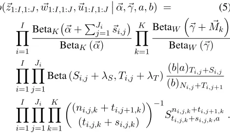
p(~z1:I,1:J, ~w1:I,1:J, ~u1:I,1:J

α, ~~ γ, a, b) = (5)

I Y

i=1

BetaK ~α+PJ_j=1i ~si,j

BetaK(~α)

K Y

k=1

BetaW

~γ+M~k

BetaW(~γ)

I Y

i=1 Ji Y

j=1

Beta(Si,j+λS, Ti,j+λT)

(b|a)Ti,j+Si,j (b)Ni,j+Ti,j+1

I Y

i=1 Ji Y

j=1 K Y

k=1

(ni,j,k+ti,j+1,k) (ti,j,k+si,j,k)

−1

S_tn_i,j,ki,j,k₊+_st_i,j,ki,j+1_,a,k .

And the following constraints apply:

ti,j,k+si,j,k≤ni,j,k+ti,j+1,k, (6)

ti,j,k+si,j,k = 0iffni,j,k+ti,j+1,k = 0. (7)

set ti,Ji+1,k = 0 (there is no Ji + 1segment) and

ti,1,k = 0(the first segment only uses~µi).

Now let us consider again the table indicators

ui,j,lfor wordwi,j,l. If this word is in topickat

doc-umentiand segmentj, then it contributes a count to

ni,j,k. It also indicates if it contributes a new table,

or a count to t0_i,j,k for the PDP at this node. How-ever, as we discussed above, this then contributes to either ti,j,k orsi,j,k. If it contributes to ti,j,k, then

it recurses up to contribute a data count to the PDP for documentisegmentj−1. Thus it also needs a table indicator at that node. Consequently, the table indicatorui,j,l for wordwi,j,l must specify whether

it contributes a table to all PDP nodes reachable by it in the graph.

We define ui,j,l specifically as ui,j,l = (u1, u2)

such that u1 ∈ [−1,0,1]andu2 ∈ [1,· · · , j],

where u2 indicates segment denoted by node νj

up to which wi,j,l contributes a table. Given u2,

u1 =−1denoteswi,j,l contributes a table count to

si,u2,k andti,j0,k foru2 < j

0 _{≤ j;u}

1 = 0denotes

wi,j,ldoes not contribute a table to nodeu2, but

con-tributes a table count toti,j0_,k foru₂ < j0 ≤j; and

u1 = 1 denotes wi,j,l contributes a table count to

eachti,j0_,kforu₂≤j0 ≤j.

Now, we are ready to compute the conditional probabilities for jointly sampling topics and table in-dicators from the model posterior of Equation (5).

5 Gibbs Sampling Algorithm

The Gibbs sampler iterates over words, doing a blocked sample of(zi,j,l, ui,j,l). The first task is to

reconstructui,j,lsince it is not stored. Since the

pos-terior of Equation (5) does not explicitly mention the ui,j,l’s, they occur indirectly through the table

counts, and we can randomly reconstruct them by sampling them uniformly from the space of possi-bilities. Following this, we then remove the values

(zi,j,l, ui,j,l) from the full set of statistics. Finally,

we block sample new values for (zi,j,l, ui,j,l) and

add them to the statistics. The new ui,j,l is

subse-quently forgotten and thezi,j,l recorded.

Reconstructing table indicatorui,j,l: We start at

the node indexedi, j. Ifsi,j,k+ti,j,k = 1andni,j,k+

ti,j+1,k > 1 then no tables can be removed since

there is only one table but several customers at the table. Thusui,j,l = (u1, u2) = (0, j)and there is no

sampling. Otherwise, by symmetry arguments, we sampleu1via

p(u1=−1,0,1|u2 =j, zi,j,l=k) ∝

(si,j,k, ti,j,k, ni,j,k+ti,j+1,k−si,j,k−ti,j,k),

since there areni,j,k+ti,j+1,kdata distributed across

the three possibilities. If after samplingu1 = −1,

the data contributes a table count up to ~µi and so

ui,j,l = (u1, u2) = (−1, j). Ifu1 = 0, theui,j,l =

(u1, u2) = (0, j). Otherwise, the data contributes a

table count up to the parent PDP for~νi,j−1 and we

recurse, repeating the sampling process at the parent node. Note, however, that the table indicator(0, j0)

forj0 < jis equivalent to the table indicator(1, j0+ 1)as far as statistics is concerned.

Block sampling(zi,j,l, ui,j,l): The full set of

pos-sibilities are, for each possible topiczi,j,l =k:

• no tables are created, soui,j,l= (0, j),

• tables are created contributing a table count all the way up to nodej0 (≤ j)but stop at j0 and do not subsequently contribute a count to~µi, so

ui,j,l = (1, j0),

• tables are created contributing a table count all the way up to nodej0 ≤ j but stop at j0 and also subsequently contribute a count to~µi, so

ui,j,l = (−1, j0).

These three possibilities lead to detailed but fairly straight forward changes to the posterior of Equa-tion (5). Thus a full blocked sampler for(zi,j,l, ui,j,l)

can be constructed.

Estimates: learnt values of~µi,~νi,j,φ~kare needed

for evaluation, perplexity calculations, etc. These are estimated by taking averages after the Gibbs sampler has burnt in, using the standard posterior means for Dirichlets and Poisson-Dirichlets.

6 Experiments

Table 3: Datasets

#docs #segs #words vocab Pat-A 500 51,748 2,146,464 16,573 Pat-B 397 9,123 417,631 7,663 Pat-G06 500 11,938 655,694 6,844 Pat-H 500 11,662 562,439 10,114 Pat-F 140 3,181 166,091 4,674 Prince-C 1 26 10,588 3,292 Prince-P 1 192 10.588 3,292 Moby Dick 1 135 88,802 16,223

6.1 Datasets

For general testing, five patent datasets are ran-domly selected from U.S. patents granted in 2009 and 2010. Patents in Pat-A are selected from in-ternational patent class (IPC) “A”, which is about “HUMAN NECESSITIES”; those in Pat-B are se-lected from class “B60” about “VEHICLES IN GENERAL”; those in Pat-H are selected from class “H” about “ELECTRICITY”; those in Pat-F are selected from class “Pat-F” about “MECHAN-ICAL ENGINEERING; LIGHTING; HEATING; WEAPONS; BLASTING”; and those in Pat-G are selected from class “G06” about “COMPUTING; CALCULATING; COUNTING”. All the patents in these five datasets are split into paragraphs that are taken as segments, and the sequence of paragraphs in each patent is reserved in order to maintain the original layout. All the stop words, the top 10 com-mon words, the uncomcom-mon words (i.e., words in less than five patents) and numbers have been removed.

Two books used for more detailed investigation are “The Prince” by Niccol`o Machiavelli and “Moby Dick” by Herman Melville. They are split into chap-ters and/or paragraphs which are treated as seg-ments, and only stop-words are removed. Table 3 shows in detail the statistics of these datasets after preprocessing.

6.2 Design

Perplexity, a standard measure of dictionary-based compressibility, is used for comparison. When re-porting test perplexities, the held-out perplexity measure (Rosen-Zvi et al., 2004) is used to evaluate the generalisation capability to the unseen data. This is known to be unbiased. To compute the held-out perplexity, 20% of patents in each data set was

ran-1025 50 100 150 200 250 300

800 900 1000 1100 1200 1300

b

Perplexity

Pat−B

Pat−F

Pat−G

Pat−H

(a) fixa= 0

0.1 0.2 0.3 0.4 0.5 0.6 0.7 0.8 0.90.90.9

800 950 1100 1250

a

Perplexity

Pat−B

Pat−G

Pat−H

Pat−F

(b) fixb= 10

Figure 3: Analysis of parameters of Poisson-Dirichlet process. (a) shows how perplexity changes with b; (b) shows how it changes witha.

0 50 100 150 200 600

700 800 900 1000 1100 1200

Lamda_S

Perplexity

Pat−B Pat−F Pat−G Pat−H Pat−A

(a) fixλT = 1

0 50 100 150 200

600 700 800 900 1000 1100 1200

Lamda_T

Perplexity

Pat−A Pat−B Pat−F Pat−H Pat−G

(b) fixλS= 1

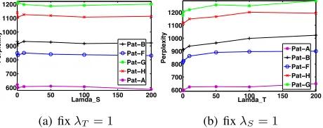
Figure 4: Analysis of the two parameters for Beta distri-bution. (a) how perplexity changes withλS; (b) how it changes withλT.

domly held out from training to be used for testing. For this, 1000 Gibbs cycles were done for burn-in followed by 500 cycles with a lag for 100 for pa-rameter estimation.

We implemented all the four models, e.g., LDA, STM, SeqTM and AdaTM in C, and ran them on a desktop with Intel Core i5 CPU (2.8GHz×4), even though our code is not multi-threaded. Perplexity calculations, data input and handling,etc., were the same for all algorithms. We note that the current AdaTM implementation is an order of magnitude slower than regular LDA per major Gibbs cycle.

6.3 Hyper-parameters in AdaTM

Experiments on the impact of the hyper-parameters on the patent data sets were as follows: First, fixing

K = 50, the Beta parametersλT = 1andλS = 1,

optimise symmetricα, and do two variationsfix-a: a = 0.0, tryingb = 1,5,10,25, ...,300, and fix-b: b = 10, tryinga = 0.1,0.2, ...,0.9. Second, fix-λT

(fix-λS): fix a = 0.2 and λT(λS) = 1, optimise

bandα, changeλS(λT) = 0.1,1,10,50,100,200.

510 25 50 100 150 630

930 1230 1530 1830 2130 2430

Number of Topics

Perplexity

LDA_D LDA_P SeqLDA STM AdaTM

(a) Pat-A

0 510 25 50 100 150 910

1060 1210 1360 1510 1660 1810

Number of Topics

Perplexity

LDA_D LDA_P SeqLDA STM AdaTM

(b) Pat-H

510 25 50 100 150

700 850 1000 1150 1300 1450 1600

Number of Topics

Perplexity

LDA_D LDA_P SeqLDA STM AdaTM

(c) Pat-B

0 510 25 50 100 150

670 820 970 1120 1270 1420

Number of Topics

Perplexity

LDA_D LDA_P SeqLDA STM AdaTM

(d) Pat-F

0 510 25 50 100 150

910 1110 1310 1510 1710 1910

Number of Topics

Perplexity

LDA_D LDA_P SeqLDA STM AdaTM

(e) Pat-G

510 25 50 100 150

−100 15 40 65 90 115 140 160

Number of Topics

Perplexity Difference

Pat−A Pat−B Pat−F Pat−G Pat−H

(f) Shuffle

Figure 5: Perplexity comparisons.

perplexity. In contrast, Figure 3(a) shows different

bvalues significantly change perplexity. Therefore, we sought to optimiseb. The experiment of fixing

λS = 1and changingλT shows a smallλT is

pre-ferred.

6.4 Perplexity Comparison

Perplexity comparisons were done with the default settings a = 0.2, α = 0.1, γ = 0.01, λS = 1,

λT = 1 and b optimised automatically using the

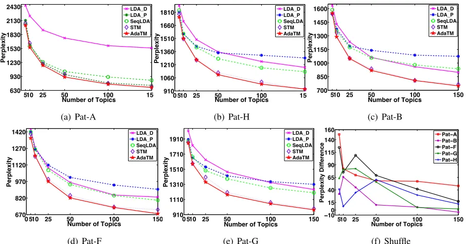
scheme from (Du et al., 2012). Figure 5 shows the results on these five patent datasets for differ-ent numbers of topics. LDA D is LDA run on whole patents, and LDA P is LDA run on the paragraphs within patents. Table 4 gives the p-values of a one-tail paired t-test for AdaTM versus the others, where lower p-value indicates AdaTM has statistically sig-nificant lower perplexity. From this we can see that AdaTM is statistically significantly better than Se-qLDA and LDA, and somewhat better than STM.

In addition, we ran another set of experiments by randomly shuffling the order of paragraphs in each patent several times before running AdaTM. Then, we calculate the difference between perplex-ities with and without random shuffle. Figure 5(f) shows the plot of differences in each data sets. The positive difference means randomly shuffling the or-der of paragraphs indeed increases the perplexity.

It can further prove that there does exist sequential topic structure in patents, which confirms the finding in (Du et al., 2012).

6.5 Topic Evolution Comparisons

All the comparison experiments reported in this sec-tion are run with 20 topics, the upper limit for easy visualisation, and without optimising any parame-ters. The Dirichlet Priors are fixed as αk = 0.1

andγw = 0.01. For AdaTM, SeqLDA, and STM,

a= 0.0andb= 100for “The Prince” andb= 200

for “Moby Dick”. These settings have proven ro-bust in experiments. To align the topics so visual-isations match, the sequential models are initialised using an LDA model built at the chapter level. More-over, all the models are run at both the chapter and the paragraph level. With the common initialisation, both paragraph level and chapter level models can

Table 4: P-values for one-tail paired t-test on the five patent datasets.

AdaTM

(a) Evolution of paragraph topics for LDA

(b) Topic alignment of LDA versus AdaTM top-ics for chapters

Figure 6: Analysis on “The Prince”.

be aligned.

To visualise topic evolution, we use a plot with one colour per topic displayed over the sequence. Figure 6(a) shows this for LDA run on paragraphs of “The Prince”. The proportion of 20 topics is the Y-axis, spread across the unit interval. The para-graphs run along the X-axis, so the topic evolution is clearly displayed. One can see there is no se-quential structure in this derived by the LDA model, and similar plots result from “Moby Dick” for LDA. Figure 6(b) shows the alignment of topics between the initialising model (LDA+chapters) and AdaTM run on chapters. Each point in the matrix gives the Hellinger distance between the corresponding top-ics, color coded. The plots for the other models, chapters or paragraphs, are similar so plots like Fig-ure 6(a) for the other models can be meaningfully compared.

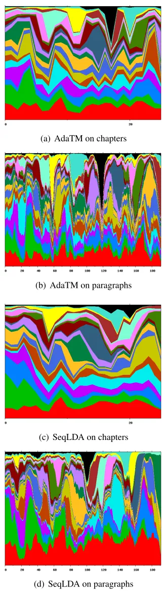
Figure 7 then shows the corresponding evolution plots for AdaTM and SeqLDA on chapters and para-graphs. The contrast of these with LDA is stark. The large improvement in perplexity for AdaTM (see Section 6.4) along with no change in lexi-cal coherence (see Section 6.2) means that the

se-(a) AdaTM on chapters

(b) AdaTM on paragraphs

(c) SeqLDA on chapters

(d) SeqLDA on paragraphs

Figure 7: Topic Evolution on “The Prince”.

(a) LDA on chapters

(b) STM on Chapters

(c) AdaTM on Chapters

Figure 8: Topic Evolution on “Moby Dick”.

figures has significantly worse test perplexity, so its sequential affect is too strong and harming results. Also, note that some topics have different time se-quence profiles between AdaTM and SeqLDA. In-deed, inspection of the top words for each show these topics differ somewhat. So while the LDA to AdaTM/SeqLDA topic correspondences are quite good due to the use of LDA initialisation, the cor-respondences between AdaTM and SeqLDA have degraded. We see that AdaTM has nearly as good sequential characteristics as SeqLDA. Furthermore, segment topic distributionνi,j of SeqLDA are

grad-ually deviating from the document topic distribution

µi, which is not the case for AdaTM.

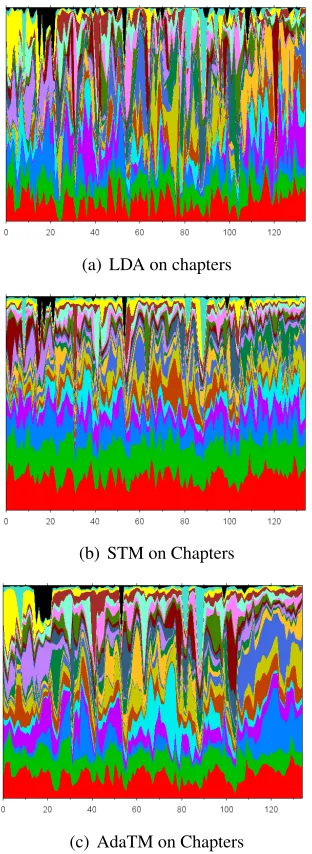
Results for “Moby Dick” on chapters are com-parable. Figure 8 shows similar topic evolution plots for LDA, STM and AdaTM. In contrast, the AdaTM topic evolutions are much clearer for the less frequent topics, as shown in Figure 8(c). Var-ious parts of this are readily interpreted from the storyline. Here we briefly discuss topics by their colour: black: Captain Peleg and the business of signing on; yellow: inns, housing, bed; mauve:

Queequeg; azure: (around chapters 60-80) details of whalesaqua: (peaks at 8, 82, 88) pulpit, schools and mythology of whaling.

We see that AdaTM can be used to understand the topics with regards to the sequential structure of a book. In contrast, the sequential nature for LDA and STM is lost in the noise. It can be very interesting to apply the proposed topic models to some text anal-ysis tasks, such as topic segmentation, summarisa-tion, and semantic title evaluasummarisa-tion, which are subject to our future work.

7 Conclusion

A model for adaptive sequential topic modelling has been developed to improve over a simple exchange-able segments model STM (Du et al., 2010) and a naive sequential model SeqLDA (Du et al., 2012) in terms of perplexity and its confirmed ability to un-cover sequential structure in the topics. One could extract meaningful topics from a book like Herman Melville’s “Moby Dick” and concurrently gain their sequential profile. The current Gibbs sampler is slower than regular LDA, so future work is to speed up the algorithm.

Acknowledgments

References

R. Arora and B. Ravindran. 2008. Latent Dirichlet allo-cation and singular value decomposition based multi-document summarization. In ICDM ’08: Proc. of 2008 Eighth IEEE Inter. Conf. on Data Mining, pages 713–718.

R. Barzilay and L. Lee. 2004. Catching the drift: Prob-abilistic content models, with applications to genera-tion and summarizagenera-tion. InHLT-NAACL 2004: Main Proceedings, pages 113–120. Association for Compu-tational Linguistics.

D.M. Blei and J.D. Lafferty. 2006. Dynamic topic mod-els. InICML ’06: Proc. of 23rd international confer-ence on Machine learning, pages 113–120.

D.M. Blei and P.J. Moreno. 2001. Topic segmenta-tion with an aspect hidden Markov model. In Proc. of 24th annual international ACM SIGIR conference on Research and development in information retrieval, pages 343–348.

D.M. Blei, A.Y. Ng, and M.I. Jordan. 2003. Latent Dirichlet allocation. Journal of Machine Learning Re-search, 3:993–1022.

W. Buntine and M. Hutter. 2012. A Bayesian view of the Poisson-Dirichlet process. Technical Report arXiv:1007.0296v2,ArXiv, Cornell, February. H. Chen, S.R.K. Branavan, R. Barzilay, and D.R. Karger.

2009. Global models of document structure using la-tent permutations. In Proceedings of Human Lan-guage Technologies: The 2009 Annual Conf. of the North American Chapter of the Association for Com-putational Linguistics, pages 371–379, Stroudsburg, PA, USA. Association for Computational Linguistics. C. Chen, L. Du, and W. Buntine. 2011. Sampling for the

Poisson-Dirichlet process. InEuropean Conf. on Ma-chine Learning and Principles and Practice of Knowl-edge Discovery in Database, pages 296–311.

S.C. Deerwester, S.T. Dumais, T.K. Landauer, G.W. Fur-nas, and R.A. Harshman. 1990. Indexing by latent semantic analysis. Journal of the American Society of Information Science, 41(6):391–407.

L. Du, W. Buntine, and H. Jin. 2010. A segmented topic model based on the two-parameter Poisson-Dirichlet process.Machine Learning, 81:5–19.

L. Du, W. Buntine, H. Jin, and C. Chen. 2012. Sequential latent dirichlet allocation.Knowledge and Information Systems, 31(3):475–503.

J. Eisenstein and R. Barzilay. 2008. Bayesian unsuper-vised topic segmentation. InProc. of Conf. on Empir-ical Methods in Natural Language Processing, pages 334–343. Association for Computational Linguistics. T.L. Griffiths, M. Steyvers, D.M. Blei, and J.B.

Tenen-baum. 2005. Integrating topics and syntax. In Ad-vances in Neural Information Processing Systems 17, pages 537–544.

A. Gruber, Y. Weiss, and M. Rosen-Zvi. 2007. Hidden topic markov models. Journal of Machine Learning Research - Proceedings Track, 2:163–170.

E.A. Hardisty, J. Boyd-Graber, and P. Resnik. 2010. Modeling perspective using adaptor grammars. In

Proc. of the 2010 Conf. on Empirical Methods in Nat-ural Language Processing, pages 284–292, Strouds-burg, PA, USA. Association for Computational Lin-guistics.

M. Johnson. 2010. PCFGs, topic models, adaptor gram-mars and learning topical collocations and the struc-ture of proper names. InProc. of 48th Annual Meeting of the ACL, pages 1148–1157, Uppsala, Sweden, July. Association for Computational Linguistics.

H. Misra, F. Yvon, O. Capp, and J. Jose. 2011. Text seg-mentation: A topic modeling perspective. Information Processing & Management, 47(4):528–544.

D. Newman, J.H. Lau, K. Grieser, and T. Baldwin. 2010. Automatic evaluation of topic coherence. In North American Chapter of the Association for Computa-tional Linguistics - Human Language Technologies, pages 100–108.

D. Newman, E.V. Bonilla, and W. Buntine. 2011. Im-proving topic coherence with regularized topic mod-els. In J. Shawe-Taylor, R.S. Zemel, P. Bartlett, F.C.N. Pereira, and K.Q. Weinberger, editors, Ad-vances in Neural Information Processing Systems 24, pages 496–504.

C.P. Robert and G. Casella. 2004. Monte Carlo statisti-cal methods. Springer. second edition.

M. Rosen-Zvi, T. Griffiths, M. Steyvers, and P. Smyth. 2004. The author-topic model for authors and docu-ments. InProc. of 20th conference on Uncertainty in Artificial Intelligence, pages 487–494.

Y. W. Teh, M. I. Jordan, M. J. Beal, and D. M. Blei. 2006. Hierarchical Dirichlet processes. Journal of the Amer-ican Statistical Association, 101:1566–1581.

Y. W. Teh. 2006. A hierarchical Bayesian language model based on Pitman-Yor processes. In Proc. of 21st Inter. Conf. on Computational Linguistics and the 44th annual meeting of the Association for Computa-tional Linguistics, pages 985–992.

H. Wallach, D. Mimno, and A. McCallum. 2009. Re-thinking LDA: Why priors matter. In Advances in Neural Information Processing Systems 19.