Abstract—Since real manufacturing is dynamic and tends to
suffer a wide range of uncertainties, research on production scheduling with uncertainty has received much more attention recently. Although various approaches have been investigated on the scheduling problem with uncertainty, this problem is still difficult to be solved optimally by any single approach, because of its inherent difficulties. This paper considers makespan optimization of a flexible flow shop (FFS) scheduling problem with stochastic processing times. It proposes a novel decomposition-based algorithm (DBA) to decompose an FFS into several clusters which can be solved more easily by different approaches. A neighbouring K-means clustering algorithm is developed to firstly group the machines of an FFS into an appropriate number of clusters, based on weighted cluster validity indices. A back propagation network (BPN) is then adopted to assign either the shortest processing time (SPT) or the genetic algorithm (GA) to generate a sub-schedule for each cluster. If two neighbouring clusters are allocated with the same approach, they are subsequently merged. After machine grouping and approach assignment, an overall schedule is generated by integrating the sub-schedules of the clusters. Computation results reveal that the proposed approach is superior to SPT and GA alone for FFS scheduling with stochastic processing times.
Keywords—back propagation network, decomposition,
flexible flow shop, neighbouring K-means clustering algorithm, stochastic processing times.
I. INTRODUCTION
Ever since the flexible flow shop (FFS) scheduling problem was identified in 1970’s [1], it has attracted considerable attention during the past decades [2]. An FFS consists of a series of production stages, each of which has several functionally identical machines operating in parallel. All the jobs released to an FFS have to visit all the stages in the same order. Research efforts on FFS scheduling problems generally consider a static environment with no unexpected events that would influence the job processing when the schedule is executed.
Real manufacturing, however, is dynamic and tends to suffer a wide range of uncertainties, such as stochastic processing times, machine breakdown, rush orders, job cancellations, and change of due date. This paper is primarily concerned with the scheduling problem of flexible flow shop with stochastic processing times. The flexible flow shop (FFS) scheduling problem [3] has been proven NP-hard in
Manuscript received June 17, 2009.
K. Wang is with the Department of Industrial and Manufacturing Systems Engineering, The University of Hong Kong, Hong Kong, China (phone: 852-6874-0287; e-mail: [email protected]).
S. H. Choi is with the Department of Industrial and Manufacturing Systems Engineering, The University of Hong Kong, Hong Kong, China (e-mail: [email protected]).
nature which is difficult to solve [4, 5]. Consideration of stochastic processing times aggravates its complexity.
As a research issue, production scheduling with uncertainty has indeed drawn considerable attention in recent years. The completely reactive approach, the robust approach, and the predictive-reactive approach are three fundamental ways [6, 7] to tackle this issue.
The completely reactive approach changes decisions during execution when necessary. The dispatching rule is a typical reactive one, in which jobs are selected by sorting them according to predefined criteria. It is easy to understand, and can find a reasonably good solution in a relatively short time. However, it uses only local information to generate a schedule which may not be globally optimal in nature. Hunsucker and Shah [8] compared the performance of dispatching rules in a constrained multiprocessor flow shop, and concluded that the Shortest Processing Time (SPT) algorithm was superior for the makespan criterion.
The robust scheduling approach takes into account possible uncertainties to construct solutions. Uncertainties, known as a priori, can be modelled by some random variables [9]. If such uncertainties are difficult to quantify, a range of scenarios will be considered and a solution is developed to optimize the performance under different scenarios [10]. In this case, the approach is viewed as a form of under-capacity scheduling to maintain robustness under different scenarios.
The predictive-reactive approach is indeed a two-step process. First, a predictive schedule is generated over the time horizon considered. This schedule is then rescheduled during execution in response to unexpected disruption. This approach is by far the most studied. The most common rescheduling methods include the right-shift schedule repair, the partial schedule repair, and the completed scheduling [11]. The right-shift schedule repair postpones the remaining operations by the amount of time needed to make the schedule feasible. The partial schedule repair only reschedules the operations that are affected by the disruption. The completed scheduling regenerates a completely new schedule for all the unprocessed operations. Although the completed scheduling may construct a better solution in theory, it is rarely applied in practice due to high computation burden and increasing scheduling instability [9]. Conversely, the right-shift schedule repair yields the least scheduling instability with the lowest computation effort, while the partial schedule repair is a moderate one in this regard.
Since each of these three approaches has its own strength and weakness, some research work has focused on comparing their effectiveness. Lawrence and Sewell [12] studied the static and dynamic applications of heuristic approach to job shop scheduling problems when processing times are uncertain. Experiment results indicated that the predictive
A Decomposition-Based Algorithm for Flexible Flow
Shop Scheduling with Stochastic Processing Times
methods based on overall information were highly likely to perform better than completely reactive approaches in an environment with little uncertainty. However, the predictive methods might lead to poor result when the uncertainty in a system exceeds a certain level.
In order to handle a complex environment, it is beneficial and imperative to take advantage of mixing these three approaches to deal with uncertainty. Matsuura et al. [13] developed a predictive approach on a periodic basis, called switching. The system switched to using a dispatching rule for the remaining operations when the deviation between the realized and predictive schedule exceeded a certain level. They concluded that the proposed approach dominated the dispatching rules when the frequency of disruption was low, but it yielded worse results than the dispatching rules when the disruption reached some level. A search of available literature indicates not much research works have been attempted to address the combination of different approaches. This paper studies the problem of scheduling an FFS with stochastic processing times. The objective is to minimize the makespan. Enlightened by the work of Lawrence’s [12], a decomposition-based algorithm (DBA) is proposed. In this approach, a neighbouring K-means clustering algorithm first groups the machines of an FFS into several clusters based on their stochastic nature when processing jobs. Then the completely reactive approach or the predictive-reactive approach, determined by the process of approach assignment, is employed to generate a sub-schedule for each cluster. Finally these sub-schedules are integrated into an overall solution.
This study contributes to the development of an integrated approach that combines and takes advantage of the completely reactive approach with the predictive-reactive approach, to deal with the uncertainty. On the contrary, the techniques reported in available literature on scheduling with uncertainty were mostly based on a single approach, yielding some initial yet limited performance. The proposed DBA explores a new direction for future research in the field of scheduling with uncertainty.
The remaining part of this paper is organized as follows. Section II is devoted to problem description. Section III describes the framework of DBA, while it is explained in detail in Section IV. To evaluate the effectiveness of DBA, simulation is conducted and computation results are analyzed in Section V. Finally, conclusions are summarized and some directions of future work are discussed in Section VI.
II. PROBLEM DESCRIPTION
In the FFS discussed above, machines sharing a similar characteristic are arranged into stages in series. Jobs have to pass all the stages in the same order. In each stage, there are a number of functionally identical machines in parallel, and a job is to be processed on one of these machines. The processing time may be highly uncertain due to quality problems, equipment downtime, tool wear, and operator availability [12]. The stochastic processing time can be described by the expected processing time E[P] and the standard deviation σ. The coefficient of processing time
variation (CPTV), defined asCPTV =σ E P
( )
, can be usedas an indicator to processing time uncertainty; it equals 0 when processing times are deterministic, and increases as the
uncertainty increases.
In order to simplify the typical FFS scheduling problem in consideration of stochastic processing times, the following assumptions are made: (1) Preemption is not allowed for job processing; (2) Each machine can process at most one operation at a time; (3) All jobs are released at the same time for the first stage; (4) There is no travel time between machines; (5) There is no setup time for job processing; (6) Infinite buffers exist for machines; (7) For the same job, the expected processing time at any parallel machine at a stage is identical; (8) The actual processing time of a job on a machine is uncertain; and (9) As parallel machines at a stage are functionally identical, they lead to the same CPTV when processing any jobs, but the CPTV may be different for other stages.
The scheduling objective under consideration is to determine the processing sequence of operations on each machine such that the makespan, which is equivalent to the completion time of the last job to leave the FFS, is minimized without violating any of the assumptions above. This FFS scheduling problem can also be described as follows.
min{max[Ct j] } (1)
Subject to the following constraints: 1
1 1 1
1
, 0
m
j j ij
i
C P if U
=
=
∑
> (2)(
)
1 1
2 1 2 1 2 2
2
1 1 1 1 1
1 1 1
, 0
m n m
j ij j j j ij
i j i
C B C P if U
= = =
=
∑ ∑
× +∑
= (3)( )-1
1 , 1 & k 0
m
kj k j kj kij
i
C C P if k U
=
= + >
∑
> (4)(
)
( )2 1 2 1 2 2
2
2 -1 1 1
1
max{ , } ,
1 & 0 k
k
m n
kj kij j kj k j kj
i j
m
kij i
C B C C P
if k U
= =
=
= × +
> =
∑ ∑
∑
(5)
0
k ij
S T ≥ (6)
(
)
1 2 1, 2
ki j ki j kj k
P =P =P, i i ∈M (7)
(k 1)i j1 ki j2 ki j2
ST + −ST ≥P (8)
1 2 2 2 1 1
[(STkij −STkij )≥Pkij] or [(STkij −STkij)≥Pkij] (9) Where
k: stage index, 1 ≤ k ≤ t
mk: number of parallel machines at stage k
Mk: set of parallel machines at stage k
i, i1, i2: machine index, 1 ≤ i, i1, i2≤ mk
j, j1, j2: job index, 1 ≤ j, j1, j2 ≤ n
Ckj: completion time of Job j at stage k
1 2 kij j
B : a Boolean variable, 1 if Job j2 is scheduled
immediately after Job j1 on machine i at stage
k, and 0 otherwise
Ukij: a Boolean variable, 1 if Job j is the first job on
machine i at stage k, and 0 otherwise
Pkj: stochastic processing time of Job j at stage k
Pkij: stochastic processing time of Job j on
machine i at stage k
For the first stage, (2) and (3) give the completion time of the first job and that of each subsequent job on the machines, respectively. Similarly for all other stages, (4) and (5) determine the completion time of the first job and that of each subsequent job on the machines, respectively. While (6) ensures non-negative start time of job processing, (7) stipulates that each of the parallel machines at a stage takes equal time to process the same job. Lastly, (8) requires the processing sequence of each stage to satisfy the processing time, and (9) guarantees that each machine can process only one job at a time.
III. THE FRAMEWORK OF THE PROPOSED
DECOMPOSITION-BASED ALGORITHM (DBA)
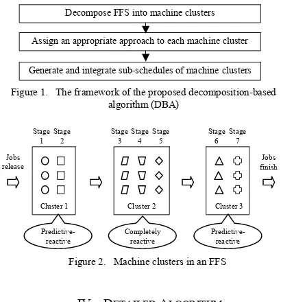
The DBA framework consists of three modules, as shown in Fig. 1. An FFS is firstly decomposed by a clustering algorithm into machine clusters, each of which contains a number of machines sharing a similar stochastic nature. As the actual processing times of jobs on a machine may be non-deterministic, the processing time uncertainty during job processing is used to describe the stochastic nature of a machine. Clustering is the classification of objects into different groups, such that the objects in each group would share some common trait. Quite a few algorithms, such as K-means, fuzzy C-means, and self-organization maps etc., have been proposed to perform the classification. Since the K-means clustering algorithm is simple and widely used, a neighbouring K-means clustering algorithm is proposed and adopted in this paper.
After decomposition of an FFS, machines in the same cluster share the similar stochastic nature of job processing and can be scheduled by the same approach. Clusters with low stochastic nature are solved by the predictive-reactive method, while those with high stochastic nature are scheduled by the completely reactive method. Due to their better performance, GA and SPT are identified as the predictive-reactive approach and the completely reactive approach, respectively. Considering the computation effort and scheduling instability, we apply right-shift scheduling repair to react to job processing delay caused by stochastic processing times.
In order to assign an appropriate approach to a machine cluster, it is critical to establish an effective model to estimate the makespan difference (MDSG) when generating the schedule by both SPT and GA. Artificial neural networks (ANNs) have been widely used in various areas due to its capability of identifying complex nonlinear relationships between input and output. The back propagation network (BPN) is a commonly used ANN structure and has been successfully applied for system modelling, prediction, and classification [14]. It is therefore adopted to determine the approach assigned to the cluster.
After approach assignment above, the sub-schedule for each of the clusters is generated by either SPT or GA, and subsequently integrated into an overall schedule. Fig. 2 shows the decomposition result of an FFS with 7 stages and 3 parallel machines at each stage. Geometric figures with the same shape represent the parallel machines. One of the two approaches, the completely reactive approach or the predictive-reactive approach, is assigned to each cluster.
IV. DETAILED ALGORITHM
A. Neighbouring K-means Clustering Algorithm
Since the CPTV represents processing time uncertainty, it is adopted to form the stochastic vector Ui to group machines
into clusters of similar stochastic natures, giving
[
]
i i
U = CPTV (10)
Where CPTVi is the CPTV of the parallel machines at stage
i. Ui represents the stochastic nature of machines at stage i. A
machine with a large CPTV indicates a high stochastic nature of job processing.
As the Euclidean distance is one of the most commonly used methods to measure the distance between a pair of data, it serves to define the machine distanceD U U
(
i, j)
, whichrepresents not the physical distance but the difference of stochastic nature between the parallel machines at stages i and j. The machine distance is calculated as follows:
(
)
(
)
22
,
i j i j i j
D U U = U −U = CPTV−CPTV (11)
ConsideringD U U
(
i, j)
, the FFS can be decomposed intomachine clusters by K-means clustering algorithm. The major problem to apply K-means clustering algorithm is the choice of cluster number. Neither a small nor a large cluster number can offer a satisfactory classification of the data objects. Recently, cluster validity indices (CVIs), indicating how well the clustering algorithm classifies the given data set, have attracted much attention as an approach to determining the optimal cluster number. Dunn [15], DB [16], Vsv [17] and DVI [18] are some typical CVIs.
However, the FFS decomposition above is different from the traditional clustering problem. Since this study aims to schedule neighbouring clusters by different approaches, a good clustering algorithm should encourage large inter-cluster distances between neighbouring clusters rather than that between non-neighbouring clusters. For this purpose, a modified DB (MDB) is proposed as follows:
1
1 n max
i j
i j
i ij ij
S S
MDB
n = ≠ W D
⎛ + ⎞
= ⎜⎜ ⎟⎟
×
⎝ ⎠
∑
(12)(
)
=1 +
ij i j
w F F (13)
Decompose FFS into machine clusters
Generate and integrate sub-schedules of machine clusters Assign an appropriate approach to each machine cluster
Cluster 1 Stage
1
Predictive- reactive
Stage 2
Cluster 2 Stage
3
Completely reactive Stage
4 Stage
5
Cluster 3 Stage
6
Predictive- reactive
Stage 7 Jobs
release
Jobs finish
[image:3.612.323.528.48.268.2]Figure 2. Machine clusters in an FFS
Where n is the number of clusters; Si denotes the average
machine distance of all objects from the cluster to their cluster centre; Dij represents the machine distance between cluster
centre i and j; Wij is the weight of Dij; Fi is the first stage of ith
cluster. A small value of MDB indicates a good clustering. In order to avoid specifying the cluster number, a neighbouring K-means clustering algorithm, incorporated with MDB, is established. Its procedure is shown in Fig. 3.
For k=2 to Kmax (Kmax = number of stages/2)
For i=1 to Imax (Imax = 10)
Apply the K-means clustering algorithm to decompose an FFS into k clusters;
Compute the MDB for ith iteration of decomposing an FFS into k clusters;
End End
Return machine clusters where the MDB is minimum over all i and all k.
B. Back Propagation Network for Approach Assignment
Under the assumptions we made on the FFS scheduling problem, jobs are released simultaneously in the first stage. However, in subsequent stages, they are allocated by the FIFO rule and may arrive non-simultaneously. Therefore, two scenarios have to be considered when establishing models to predict the MDSG. The first scenario assumes the jobs to be released simultaneously, while the other allows the jobs arrive non-simultaneously.
Accordingly, two BPNs, each corresponds to a scenario, are generated. The configurations of these BPNs are established as follows: (1) Inputs: Four parameters, namely CPTV, stage size, job size and parallel machine size. These parameters are found to affect the performance of MDSG significantly according to the experiment results in Section V; (2) Number of single hidden layers: Generally one hidden layer is capable of approximating any function with a finite number of discontinuities. Therefore, the BPN only consists of one hidden layer; (3) Number of hidden neurons: There is no concrete rule to find the optimal number. If inadequate hidden neurons are adopted, it may introduce a greater risk of modelling the complex data poorly. If too many hidden neurons are used, the network may fit the training data extremely well, but would perform poorly to new and unseen data. For these reasons, the optimum number is intentionally chosen from the interval [2, 20]. The BPNs with different number of hidden neurons are evaluated by the mean square error (MSE), and the one with the minimum MSE has the optimum number of hidden neurons; (4) Output: MDSG; (5) Number of epochs per replication: 10000; (6) Number of replications: 100. The performance of a BPN is sensitive to the initial condition of network. The network with different initial conditions will be trained and evaluated respectively. Among the results, the best one is chosen.
After training, validation, and testing, the BPNs can estimate the MDSG. If the MDSG is predicted to be positive, GA is allocated to address the scheduling problem of the cluster. Otherwise, SPT is used to generate the schedule for the cluster. However, the neighbouring K-means clustering algorithm cannot avoid the possibility that two neighbouring clusters are to be suitably solved by the same approach.
Therefore, it is reasonable to conduct a cluster merging process (CMP) to integrate neighbouring clusters if necessary, using the following steps: (1) Identify the two neighbouring clusters which are to be solved by the same approach; (2) Merge the two neighbouring clusters and determine the approach for the new cluster by BPNs; (3) Repeat steps 1 and 2 until any two neighbouring clusters are allocated with different approaches.
Integrating with CMP, the complete process of approach assignment is summarized as follows: (1) Collect the data sets for both scenarios, including CPTV, stage size, job size, parallel machine size, and the expected MDSG; (2) Train, validate and test the BPNs; (3) Estimate the MDSG for each machine cluster by BPNs; (4) Assign either SPT or GA to each machine cluster according to the positive or negative sign of its estimated MDSG, respectively; (5) Conduct CMP.
C. Cluster Scheduling
After FFS decomposition and approach assignment, sub-schedules are generated by either SPT or GA for all machine clusters and then integrated into an overall solution.
SPT performs better with low computation cost when the machines in a machine cluster with a large CPTV. It consists of the following two main steps: (1) Determine the job sequence based on the SPT rule for the first stage; (2) Allocate the finished job from the previous stage to the current stage by the FIFO rule until all the jobs are processed at each stage.
GA is used prior to the dispatching rules when scheduling a machine cluster with a small CPTV. The right-shift scheduling repair is triggered to regenerate a new schedule whenever the start time of job processing has to be postponed due to the stochastic processing times. The overall structure of our GA is briefly described as follows: (1) Coding: The job sequence is used as the chromosome for the FFS scheduling problem. For example, job sequence [2,3,5,1,4,9,8,6,7,10] is a chromosome with ten jobs in an FFS; (2) Fitness function: It is formulated as fitness = Cmax, where Cmax is the maximum
completion time of jobs; (3) Selection strategy: Roulette wheel selection is applied to reproduce the next generation; (4) Crossover and mutation operation: Order preserved crossover (OPX) and shift move mutation (SM) are adopted. The crossover rate and mutation rate are analyzed by setting different values on the same FFS scheduling problem. A crossover rate of 0.8 and a mutation rate of 0.2 are found to give good performance; (5) Termination criterion: The algorithm continues until 200 generations have been examined. This value is chosen empirically.
V. COMPUTATIONAL RESULTS AND ANALYSIS
The test-bed contains 27 problems with different stages, jobs and parallel machines, as shown in Table II. For each problem, ten instances with different expected processing times of operations are randomly generated. The actual processing time of job i on machines at stage j is stochastic and assumed to follow the gamma distribution with the expected processing time E(Pij) and standard deviation
( ij) j
E P CPTV
σ
= × , where CPTVj is the coefficient ofprocessing time variation at stage j. The simulation is iterated 50 times for each instance.
A. Establishing BPNs for MDSG Estimation
[image:5.612.70.300.166.227.2]Corresponding to the two scenarios of simultaneous and non-simultaneous job arrivals, the examples for training and testing BPNs are generated for all the problems in the test-bed. The levels of BPN input used in the experiments are shown in Table I. This results in a total of 3,600 (10×10×6×6 = 3,600) training examples.
TABLE I. BPN INPUTS AND THEIR LEVELS
Factors Levels
CPTV 10 levels (0.1, 0.2, …, 1) Stage size 10 levels (1, 2, …, 10)
Job size 20, 25, 30, 35, 40, 45 Parallel machine size 2, 3, 4, 5, 6, 7
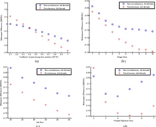
Based on the data of the examples, scatter plots are generated to visualize the relationship of four factors, including CPTV, stage size, job size and parallel machine size, on the MDSG. As shown in Fig. 4, circles and squares represent the results derived by the scenarios of simultaneous job arrivals and non-simultaneous job arrivals, respectively. Accordingly the following conclusions are drawn: (1) The MDSG decreases with the increasing of CPTV, stage size and job size. Parallel machine size affects the MDSG as well.
Therefore, it is reasonable to adopt these four factors as BPN inputs; (2) The MDSG is different for the two scenarios of simultaneous and non-simultaneous job arrivals. Hence, two BPNs are needed to estimate the MDSG.
The prediction accuracy of the two BPNs is measured by MSE. The minimal MSE with various numbers of hidden neurons in the hidden layer are compared in Fig. 5. The optimum numbers of BPNs with simultaneous and non-simultaneous job arrivals are 12 and 14, respectively. The BPNs with the optimum numbers are adopted to estimate the MDSG.
B. DBA Analysis
To evaluate the effectiveness of the proposed approach, SPT, GA, and DBA are analyzed in a stochastic environment in which CPTV is uniformly distributed in the interval [0.1, 1]. The experiment results of these three approaches with stochastic processing times (denoted by SPT_S, GA_S, and DBA_S respectively) are shown in Table II. The results of SPT and G A with deterministic processing times (denoted by SPT, and GA respectively) are also given. It can be seen that DBA_S gives the best performance in most cases, decreasing the makespan by about 3% and 8% in comparison with SPT_S and GA_S, respectively.
0.1 0.2 0.3 0.4 0.5 0.6 0.7 0.8 0.9 1
-0.4 -0.3 -0.2 -0.1 0 0.1 0.2 0.3
Coefficient of processing time variation (CPTV)
M
ak
es
pan D
if
fer
enc
e (M
D
S
G)
Non-simultaneous Job Arrivals Simultaneous Job Arrivals
1 2 3 4 5 6 7 8 9 10
-0.18 -0.16 -0.14 -0.12 -0.1 -0.08 -0.06 -0.04
Stage Size
M
a
k
e
s
p
an D
if
fe
re
nc
e (
M
DS
G
)
Non-simultaneous Job Arrivals Simultaneous Job Arrivals
(a) (b)
20 25 30 35 40 45
-0.17 -0.16 -0.15 -0.14 -0.13 -0.12 -0.11 -0.1 -0.09 -0.08 -0.07
Job Size
M
ak
es
p
an D
if
fer
e
nc
e (
M
D
S
G
)
Non-simultaneous Job Arrivals Simultaneous Job Arrivals
2 3 4 5 6 7
-0.16 -0.15 -0.14 -0.13 -0.12 -0.11 -0.1 -0.09 -0.08 -0.07
Parallel Machine Size
M
a
k
e
s
pan Di
ff
er
enc
e (
M
DS
G
)
Non-simultaneous Job Arrivals Simultaneous Job Arrivals
[image:5.612.148.455.340.591.2](c) (d)
Figure 4. Scatter plots of the MDSG with (a) coefficient of processing times (CPTV), (b) stage size, (c) job size, (d) parallel machine size.
2 4 6 8 10 12 14 16 18 20
0.6 0.8 1 1.2 1.4 1.6
1.8x 10
-3
Number of hidden neurons
Mi
n
imu
m MS
E
2 4 6 8 10 12 14 16 18 20
3 3.5 4 4.5 5 5.5 6
6.5x 10
-4
Number of hidden neurons
Mi
n
imu
m MS
E
(a) (b)
TABLE II. COMPARISON OF PERFORMANCE OF VARIOUS SCHEDULING ALGORITHMS a
Problem size (No. of jobs x no. of stages) No. of Parallel Machines in each stage SPT GA SPT_S GA_S DBA_S
20×6 2 1.170 1.000 1.318 1.384 1.257
20×6 3 1.202 1.000 1.345 1.395 1.276
20×6 4 1.220 1.000 1.396 1.557 1.350
20×10 2 1.120 1.000 1.321 1.450 1.305
20×10 3 1.165 1.000 1.296 1.409 1.277
20×10 4 1.119 1.000 1.302 1.504 1.292
20×15 2 1.144 1.000 1.290 1.413 1.255
20×15 3 1.114 1.000 1.265 1.459 1.246
20×15 4 1.083 1.000 1.170 1.295 1.158
30×6 2 1.099 1.000 1.246 1.358 1.212
30×6 3 1.165 1.000 1.309 1.415 1.246
30×6 4 1.163 1.000 1.341 1.535 1.271
30×10 2 1.135 1.000 1.320 1.459 1.298
30×10 3 1.153 1.000 1.287 1.425 1.249
30×10 4 1.121 1.000 1.279 1.504 1.280
30×15 2 1.157 1.000 1.291 1.404 1.261
30×15 3 1.159 1.000 1.284 1.475 1.255
30×15 4 1.125 1.000 1.295 1.499 1.279
40×6 2 1.134 1.000 1.242 1.265 1.199
40×6 3 1.129 1.000 1.257 1.354 1.188
40×6 4 1.139 1.000 1.296 1.514 1.291
40×10 2 1.165 1.000 1.314 1.375 1.249
40×10 3 1.158 1.000 1.326 1.508 1.256
40×10 4 1.086 1.000 1.266 1.528 1.252
40×15 2 1.147 1.000 1.297 1.402 1.255
40×15 3 1.116 1.000 1.265 1.472 1.237
40×15 4 1.118 1.000 1.276 1.538 1.272
Average 1.141 1.000 1.292 1.441 1.258
a. All the results are the ratios of the average makespan of various scheduling algorithms to that of GA.
VI. CONCLUSION
This paper proposed a decomposition-based algorithm (DBA) to makespan optimization of an FFS scheduling problem with stochastic processing times. In this approach, machines are grouped into several clusters by a neighbouring K-means clustering algorithm without predefining the number of clusters, and each cluster is scheduled by either SPT or GA.
The effectiveness of DBA was validated with experiment results. For most problems in the test-bed, DBA is superior to SPT and GA. The better performance of DBA results from the decomposition strategy – to schedule with GA in a low stochastic environment and with SPT in a high stochastic environment. This strategy ensures DBA’s good performance when addressing FFS scheduling problems in any stochastic environment.
The proposed DBA provides a promising way to address the FFS scheduling problem with stochastic processing times. Further research can be devoted to evaluating the performance of DBA by optimizing the FFS scheduling problem for tardiness related criteria, such as minimizing the mean tardiness of jobs.
REFERENCES
[1] T. S. Arthanari and K. S. Ramamurthy, "An extension of two machines sequencing problem," Opsearch, 8, pp. 10-22, 1971.
[2] H. Wang. "Flexible flow shop scheduling: optimum, heuristics and artificial intelligence solutions," Expert Systems, 22(2), 78-85, 2005. [3] R. Linn and W. Zhang, "Hybrid flow shop scheduling: a survey,"
Computers and Industrial Engineering, vol. 37, pp. 57-61, 1999. [4] M. R. Garey, Computers and intractability: a guide to the theory of
NP-completeness. New York: W. H. Freeman, 1979.
[5] J. N. D. Gupta, "Two-stage, hybrid flowshop scheduling problem," Journal of the Operational Research Society, vol. 39, pp. 359-364, 1988.
[6] H. Aytug, M. A. Lawley, K. McKay, S. Mohan, and R. Uzsoy, "Executing production schedules in the face of uncertainties: A review and some future directions," European Journal of Operational Research, vol. 161, pp. 86-110, 2005.
[7] T. Vidal, "The many ways of facing temporal uncertainty in planning and scheduling," Tatihou, France, 2004, pp. 9-12.
[8] J. L. Hunsucker and J. R. Shah, "Comparative performance analysis of priority rules in a constrained flow shop with multiple processors environment," European Journal of Operational Research, vol. 72, pp. 102-114,1994.
[9] L. Liu, H. Y. Gu, and Y. G. Xi, "Robust and stable scheduling of a single machine with random machine breakdowns," The International Journal of Advanced Manufacturing Technology, vol. 31, pp. 645-654, 2007.
[10] P. Kouvelis, R. L. Daniels, and G. Vairaktarakis, "Robust scheduling of a two-machine flow shop with uncertain processing times," IIE Transactions, vol. 32, pp. 421-432, 2000.
[11] G. E. Vieira, J. W. Herrmann, and E. Lin, "Rescheduling manufacturing systems: A framework of strategies, policies, and methods," Journal of Scheduling, vol. 6, pp. 39-62, 2003.
[12] S. R. Lawrence and E. C. Sewell, "Heuristic, optimal, static, and dynamic schedules when processing times are uncertain," Journal of Operations Management, vol. 15, pp. 71-82, 1997.
[13] H. Matsuura, H. Tsubone, and M. Kanezashi, "Sequencing, dispatching, and switching in a dynamic manufacturing environment," International Journal of Production Research, vol. 31, pp. 1671-1688, 1993. [14] D. Y. Lin and S. L. Hwang, "Use of neural networks to achieve
dynamic task allocation: a flexible manufacturing system example," International Journal of Industrial Ergonomics, 24(3), 281-298, 1999. [15] J. C. Dunn, "Fuzzy relative of iosdata process and its use in detecting
compact well-separated clusters," J Cybern, vol. 3, pp. 32-57, 1973. [16] D. L. Davies and D. W. Bouldin, "A Cluster Separation Measure,"
Pattern Analysis and Machine Intelligence, IEEE Transactions on, vol. PAMI-1, pp. 224-227, 1979.
[17] D. J. Kim, Y. W. Park, and D. J. Park, "A novel validity index for determination of the optimal number of clusters," IEICE Transactions on Information and Systems, vol. E84-D, pp. 281-285, 2001. [18] J. Shen, S. I. Chang, E. S. Lee, Y. Deng, and S. J. Brown,