Robust Design Guidelines for Model Reference
Adaptive Control
L. Yang, S.A. Neild, and D.J. Wagg
∗ [image:1.595.327.531.205.307.2]Abstract–In this paper a robust design process is in-troduced for a scalar model reference adaptive control (MRAC) algorithm. Three different types of MRAC control rules are reviewed and analysed in the fre-quency domain. A design process for MRAC is given within the range of plant settling times 0.01-100 sec-onds which is relevant for a wide range of mechanical systems. By using this design method the MRAC system stability can be made robust in the presence of a range of disturbances or plant uncertainties. An example of applying this method to hydraulic shaking table model with unmodelled oil column resonance is given at the end.
Keywords: Adaptive control, Nonlinear dynamics, Gain wind-up, Robustness, Stability, Tuning method
1
Introduction
In this paper a robust design process is introduced for a scalar MRAC algorithm, which can ensure a robust control system within a large frequency range. Our in-tention is to provide a series of control design guidelines for the scalar MRAC system so that robust design can be achieved for a range of mechanical plants. Detailed dis-cussions on MRAC are given by [1, 2, 3]. This work builds on the previous work on modifying the MRAC algorithm to improve robustness [4, 5]. The formulations of MRAC will be reviewed in section 2. Five different MRAC adap-tive gain rules will be studied in section 3. In section 4 the robust design process will be explained step by step, and finally an example by applying this design process will be given in section 5.
2
MRAC brief review
In this section a brief review of the MRAC method is given for a single input single output (SISO) system. For more detailed discussions of MRAC see [1, 2, 3].
The system studied in this paper is based on a first-order linear plant approximation given by
˙
x(t) =−ax(t) +bu(t), (1)
∗Department of Mechanical Engineering, University of
Bris-tol, Queens Building, University Walk,Bristol BS8 1TR, U.K. Email: [email protected]
K
Reference Model xm= -am*xm+bm*r
.
Adaptive Algorithm ++
Kr
+ - Ce
xm
r u=K*x+Kr*r x ye
Plant x= -a*x+b*u.
Xe
Figure 1: Schematic block diagram of the model reference adaptive control system. K and Kr are the gains from adaptive algorithm.
where x(t) is the plant state, u(t) is the control signal andaandbare the plant parameters. The control signal is generated from both the state variable and the refer-ence (or demand) signalr(t), multiplied by the adaptive control gainsKand Kr, such that
u(t) =K(t)x(t) +Kr(t)r(t), (2)
where, K(t) is the feedback adaptive gain andKr(t) the feed forward adaptive gain. The plant is controlled to follow the output from a reference model
˙
xm(t) =−amxm(t) +bmr(t), (3)
wherexmis the state of the reference model andamand
bmare the reference model parameters which are specified by the controller designer. The block diagram of MRAC is illustrated by Fig. 1.
The object of the MRAC algorithm is for xe → 0 as
t → ∞, where xe = xm−x is the error signal. The
dynamics of the system can be rewritten in terms of the error such that
˙
xe= (−a+bK)xe+b(KE−K)xm+b(KrE−Kr)r, (4)
where KE andKE
r are Erzberger gains. The Erzberger gains are defined as the linear gains which results in the plant response matching the reference model response [6]:
KE= a−am
b , K
E r =
bm
3
Different MRAC adaptive gain rules
In this section three different MRAC adaptive gain rules, MIT, Hyperstability and ρ φ modified MRAC version, i.e., will be reviewed, and all the control rules will be illustrated and explained based on their Bode plots.
3.1
MRAC by using the MIT rule
A basic method of MRAC adaptive gain is known as MIT rule [1], which is using an integral control in the adaptive gains, and designed by using Lyapunov stability theory. The formulation can be described as
K(t) =αR0tCexex(τ)dτ+K0,
Kr(t) =αR0tCexer(τ)dτ+Kr0,
(6)
whereαis adaptive control weight representing the adap-tive effort andK0andKr0are the initial gain values and
Ce can be chosen to ensure the stability of the feed for-ward block [2]. In the case of a first-order implementa-tion, Ce is a scalar and therefore may be incorporated into theαadaptive control weight.
In general the initial gain values,K0andKr0, can be set to zero such that the controller requires no knowledge of the plant parametersaandb [7] — although this gener-ally leads to slower convergence to final gain values, or the Erzberger gains estimated based on a first-order system identification of the plant. The adaptive weight,αneed to be selected in advance, and clearly have a significant influence on the rate of adaptation.
By using Laplace transform given zero initial conditions, Eq. 6 becomes,
(K(s)−K0)/P1(s) =α/s,
(Kr(s)−Kr0)/P2(s) =α/s, (7)
wheresis the Laplace transform variable and
P1(s) =CeXe(s)X(s),
P2(s) =CeXe(s)R(s). (8)
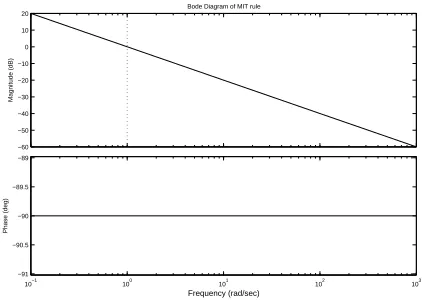
If P1 or P2 is considered as overall input signal, Eq. 8 describes the relationship between output, the adaptive gains, and input P1 andP2. As we can see the transfer function on the right hand side are identical. A point to be noted from the transfer function is that when s =α
theoutput/input= 1. In the Bode plot sincesrepresents
frequency (s =jw), at frequency of ω = αrad/sec the magnitude is 0dB. We also noticed there is a zero pole, which makes the transfer function marginally stable.
Transfer function Eq. 8 is illustrated as a Bode plot by Fig. 2. An example ofα= 1 is given in this figure. As we can see at frequency of α= 1 rad/sec the magnitude is 0dB, and the input with frequency higher than 1 rad/sec is minimised in the output signal — the adaptive control gains. This 0dB frequency can be adjusted by choosing differentαvalues.
−60 −50 −40 −30 −20 −10 0 10 20
Bode Diagram of MIT rule
Magnitude (dB)
10−1 100 101 102 103 −91
−90.5 −90 −89.5 −89
Frequency (rad/sec)
[image:2.595.322.533.73.223.2]Phase (deg)
Figure 2: Transfer function of adaptive control gain by using MIT rule (integral control), adaptive weighting
α= 1. The vertical dot line indicates at αrad/sec the magnitude is 0 dB.
3.2
MRAC by using the hyperstability rule
In most of MRAC applications, the adaptive gains defined by using Hyperstability rule are considered as a standard case. The Hyperstability rule defines the adaptive gains with a proportional plus integral formulation as
K(t) =αR0tCexex(τ)dτ+βCexex(t) +K0,
Kr(t) =αR0tCexer(τ)dτ+βCexer(t) +Kr0, (9)
where α and β are adaptive weights. In a first-order implementation Ce can be incorporated into the α and
β. The adaptive gain K(t) can be written in thes-plane by using Laplace transform as
K(s)−K0
P1(s)
=β(s+α/β)
s . (10)
The Laplace transform result ofKr(t) is identical as the right hand side of Eq. 10. To keep the description simple we only analyse the adaptive gain K. In Eq. 10 the break frequencyω=α/βrad/sec need to be noted, since a steady-state β exists in the frequency higher than this value.
Eq. 10 is illustrated by Bode plot Fig. 3. An example of α= 1,β = 0.1 is given in this figure. As we can see after the break frequency α/β = 10 rad/sec the magni-tude becomes a steady state gain of 20log10(β) =−20.
Comparing with MIT rule, the Hyperstability rule allows the designer to adjust the break frequency by usingα/β
ratio, and set theoutput/inputto a fixed magnified ratio
β in the frequency higher thanα/βrad/sec.
3.3
MRAC with
ρ φ
modification
−60 −50 −40 −30 −20 −10 0 10 20 30
40 Bode Diagram of Hyperstability rule
Magnitude (dB)
10−1 100 101 102 103 −90
−45 0
Frequency (rad/sec)
Phase (deg)
Figure 3: Transfer function of adaptive control gain by using Hyperstability rule (proportional plus integral). The vertical dot-line indicates the frequencyα/βrad/sec. The adaptive weights areα= 1, β= 0.1.
create an ‘adaptive window’ such that adaptive gain con-trol power can be focused within this frequency window. It can eliminate the adaptive control gain wind-up prob-lem caused by disturbance [8, 5] and instability probprob-lem caused by unexpected high frequency dynamics in control plant [4]. MRAC withρ φmodification can be described by equations as
Km(s) = (s+ρ2φ)(2ss+φ2)K(s) +
ρ2
s+ρ2K∗(s)
+ s2
(s+ρ2)(s+φ2)K∗(s),
Krm(s) = φ2
s
(s+ρ2)(s+φ2)Kr(s) +
ρ2
s+ρ2Kr∗(s)
+ s2
(s+ρ2)(s+φ2)Kr∗(s),
(11)
where ()mdenotes modified MRAC.ρandφare constants needed to be selected by the designer, and K∗(s) and
K∗
r(s) are steady state gains, which ideally are equal to the Erzberger Gains. K(t) andKr(t) are Hyperstability MRAC control gains described by Eq. 9.
It can be noticed from Eq. 11 that the first term on the right hand side with K(s) is the adaptive gain control part, and the second and third terms are steady-state gain control based on K∗(s). The whole structure can
be illustrated by Fig 4. An adaptive window is created betweenρ2andφ2rad/sec. The steady-state gain control is used outside the window. The ρ term cuts off the adaptive power to low frequency, and termφcuts off the adaptive power to high frequency. The same situation can be found from modified gain Krm. The following research is concerned with the adaptive gain control part. The transfer function of adaptive gain control part can be derived by substituting Eq. 10 intoKmin Eq. 11
Km(s)−K0
P1(s)
= φ
2β(s+α/β)
(s+ρ2)(s+φ2). (12)
It can be noticed from Eq. 12 that both poles−ρ2 and −φ2are negative givenρ φare non-zero. Hence the
adap-10−4 10−3 10−2 10−1 100 101 102 103 104 −40
−30 −20 −10 0 10 20
Bode Diagram of MRAC with ρ and φ modification
Frequency (rad/sec)
Magnitude (dB)
K (adaptive gain control)
K* (fixed gain control) ρ2 φ2 K* (fixed gain control)
[image:3.595.62.276.73.226.2]Adaptive window
Figure 4: The structure diagram of MRAC withρ φ mod-ification. Dash-dot line illustrates the adaptive gain trol part. Solid line illustrates the steady-state gain con-trol part. Two vertical dash line illustrate ρ2 and φ2 separately.
−60 −40 −20 0 20
Bode diagram of MRAC with ρφ modification
Magnitude (dB)
10−2 10−1 100 101 102 103 104 105 −90
−45 0 45 90
Frequency (rad/sec)
[image:3.595.323.533.74.145.2]Phase (deg)
Figure 5: Transfer function of the adaptive gain control part of MRAC by using ρ and φ modification. Vertical dash line on left and right illustrate the frequency of ρ2 and φ2 rad/sec correspondingly, and vertical dot line is the frequency of α/βrad/sec. The adaptive weights are
α= 1,β = 0.1,ρ2= 1 rad/sec andφ2= 103 rad/sec.
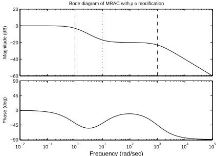
tive gain is asymptotically stable rather than marginally stable in the Hyperstability MRAC. The MRAC withρ φ
modification has three break frequenciesρ2,α/βand φ2 rad/sec. Two stead-statesα/ρ2andβ are corresponding to the frequency ranges of (0, ρ2) and (α/β, φ2). The transfer function Eq. 12 can be illustrated by Bode plot Fig. 5. Fig. 5 shows the example of ρ2 = 1,α/β = 10 andφ2= 103rad/sec. In the frequency lower thanρ2= 1 rad/sec the adaptive gain control part can be set to a steady-state ofα/ρ2= 1(0dB), and in frequency between
α/β = 10 and φ2 = 103 rad/sec the adaptive gain con-trol part can be set to the steady-stateβ = 0.1(-20dB). In frequency higher thanφ2 = 103 rad/sec the adaptive power is cut off.
Comparing with the standard MRAC strategy, the ρ φ
[image:3.595.321.532.241.393.2]4
MRAC robust design process
In this section a robust design process will be introduced by using MRAC strategy. The study here is mainly con-cerned on the plants that can be estimated by using first order transfer function, but could be combined with dis-turbance and unmodelled higher order dynamics. The design process can be taken in four steps, concerning on the plant parameter, the reference model, adaptive weights and adaptive window.
4.1
Step1:
Find out the plant break
fre-quency
a
by doing system ID within the
operation frequency
The robust MRAC design process needs to know a limited amount knowledge of the plant. This is the normal trade off between robustness andaprior knowledge.
The break frequencyaor settling timetsp, i.e.,first order plant, needs to be known or estimated. (The relationship of a = 4/tsp can be used to convert tsp to a.) Given the operation frequency range is known, aor tsp can be found out by using chirp signal to do system identifica-tion. Then the model of the first order plant can be given as X(s)/R(s) =b/(s+a).
4.2
Step2:
Decide the reference model
break frequency
am
The key parameter in the reference model is the break frequency am or settling time ts. It is possible to have reference model settling timetsslightly faster than plant settling timetsp, so that the control system can be forced to settle faster than it’s open loop response. But ifts is set too fast, the control system will become unstable [1]. The relationship betweents andtspis studied against a range of plant settling time 0.01-100 seconds, or plant break frequency 0.04-400 rad/sec. To make the results clearer in frequency domain, the ratio between tsp and
ts has been convert to the ratio of am and a, by using relationshiptsp/ts=am/a.
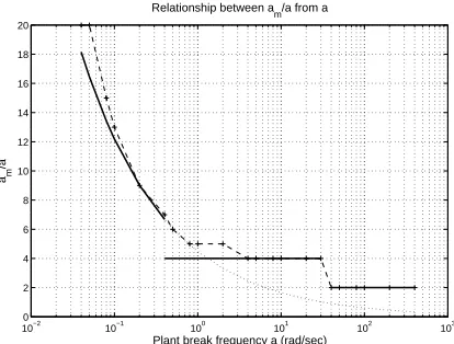
All tests in section 4 is processed using the conditions: 1) input frequency is equal to plant break frequency, 2) sam-pling time for control system is smaller than 10% plant settling time, 3) disturbance is included in the testing plant, i.e., 5% white Gaussion noise, 4) stability checked by control gains and error converge within two times plant settling time. Fig. 6 shows the relationship be-tween am/a and a. It can be noticed from Fig. 6 that as plant break frequency aincreases, am/a ratio for the stable system decrease. The recommended values in each frequency ranges are
• am/a = 4.5e−log10(a) is recommended when a ∈
(0.04 0.4)rad/sec ortsp∈(10 100)sec.
10−2
10−1
100
101
102
103
0 2 4 6 8 10 12 14 16 18 20
Plant break frequency a (rad/sec) am
/a
[image:4.595.325.532.74.231.2]Relationship between a m/a from a
Figure 6: The relationship betweenam/aand plant break frequencya. The dash-line with + marks shows the orig-inal data of am/a for stable MRAC against a rad/sec, and area below it is stable. The dot-line illustrates the exponential curve fitting. The black lines illustrate the recommended values in each frequency ranges.
• am/a= 4 is recommended whena∈(0.4 40)rad/sec
ortsp∈(0.1 10)sec.
• am/a= 2 is recommended whena∈(40 400)rad/sec
ortsp∈(0.01 0.1)sec.
The Erzberger gains can be calculated now as by Eq. 5, andK∗ andK∗
r are set to Erzberger gains.
4.3
Step3: Select adaptive weights
α,
β.
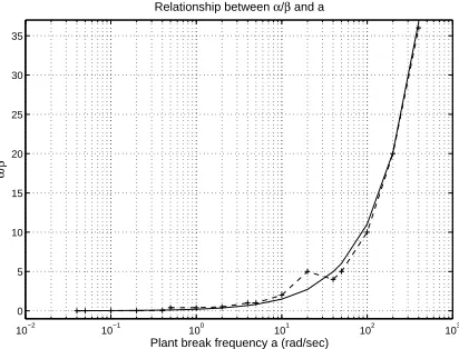
In this step we first selectα/βvalue and thenα. β value can be calculated by using α/βand α. The relationship betweenα/β andais tested in the range of plant break frequency 0.04-400 rad/sec by fixingα= 1 and checking
α/β stability value. In different frequency ranges the corresponding recommended am values are used. Fig. 7 illustrates the results. As a increases in frequency α/β
becomes large. Since α is fixed the β value decreases and the effective adaptive power decreases. It can to be noticed in Fig. 7 that the exponential equation fit well in the high frequency range of (40 400)rad/sec but not the low frequency part. Experiment results show that the following recommended values are effective to ensure the system robustness as well as small error.
• α/β=ais recommended whena∈(0.04 40)rad/sec
ortsp∈(0.1 100)sec.
• α/β = 0.2e2log10(a) is recommended when a ∈
(40 400)rad/sec ortsp∈(0.01 0.1)sec.
10−2 10−1 100 101 102 103 0
5 10 15 20 25 30 35
Plant break frequency a (rad/sec)
α
/
β
[image:5.595.68.274.75.232.2]Relationship between α/β and a
Figure 7: The relationship betweenα/βand plant break frequency a as α = 1. The dash-line with + marks shows the original data ofα/βfor stable MRAC against
a rad/sec, and area above it is stable. The solid line illustrates the exponential curve fitting with equation
α/β= 0.2e2log10(a).
into three sections, 0.04-0.4, 0.4-40 and 40-400 rad/sec, and in each section the corresponding recommended am and α/β values are used. In each section asa increases the maximal α for stable system decreases. In general as the adaptive weightαincreases control system settles fast and error decreases, but too large α will cause the system instability. One way to choose theαvalue is to use the value which gives the minimal error, as recommended here
• α= 10 is recommended when a∈(0.04 0.4)rad/sec
ortsp∈(10 100)sec.
• α = −0.15a + 10 is recommended when a ∈
(0.4 40)rad/sec ortsp∈(0.1 10)sec.
• α = −0.03a + 12 is recommended when a ∈
(40 400)rad/sec ortsp∈(0.01 0.1)sec.
Some other factors could also affect choosing the adaptive weights, the input frequencyωr, i.e. Withωrclose to the plant break frequency athe maximum adaptive weights that can be chosen for a stable system increases. But the effect was not found to be significant.
4.4
Step4: Designing the adaptive window
In this step an adaptive window will be selected, and by using this window the designer can limit the adaptive power only to the interesting frequency range, and cut off the adaptive power in both low and high frequency disturbance or unexpected dynamics, and the robustness of overall control system is ensured [4]. The principal rule of setting the adaptive window is that a, am, α/β, and input frequencyωrshould be included in the window
10−2 10−1 100 101 102 103
0 5 10 15 20 25 30 35
Plant break frequency a (rad/sec)
α
value
[image:5.595.325.533.76.231.2]Relationship between α and a
Figure 8: The relationship between α and plant break frequency a. Two vertical lines divide the whole plot into three frequency sections. In each sections different
am/a and α/βare chosen by following the previous rec-ommended values. The dash-line with + marks shows maximalαfor stable MRAC. The dot-line illustrates the
αvalues which gives minimal error. The dark-solid lines show the recommended αvalues.
defined by ρ2, φ2. The key results of this design process are summarized in table 1.
5
Experiment by using MRAC design
process
In this section an example will be given by applying the MRAC design process on a reconfigurable electrical cir-cuit, a Quansar analog plant simulator. By using it an hydraulic shaking table model is created as
G(s) = 2.108
(s+ 1.147)
229.521
(s2+ 2.895s+ 231.516), (13)
where the nominal first order plant is 2.108/(s+ 1.147), and high order dynamics part is 229.521/(s2+ 2.895s+ 231.516) which represents the oil column resonance in the hydraulic shaking table. By carrying out system identification to operation frequency range 0-10 Hz, the break frequency of the nominal plant a = 1.147 can be found. The input signal is sinusoid wave given as
r(t) = 0.3 + 1.85 sin(0.8t).
Since this plant has unmodelled high frequency dynamics and electronic noise, by using standard MRAC the con-trol system become unstable within 15 sec, Fig. 9. Using the MRAC design process, sincea∈(0.4 40)rad/sec the
following parameters can be chosen by following the de-sign process as
• am= 4a= 4,
• α/β=a= 1,
Table 1: MRAC parameter design table
Parameters Recommend values
a system ID
a∈(0.04 0.4)rad/sec
am 4.5e−log10(a)∗a
α/β a
α 10
a∈(0.4 40)rad/sec
am 4a
α/β a
α −0.15a+ 10
a∈(40 400)rad/sec
am 2a
α/β 0.2e2log10(a)∗a
α −0.03a+ 12
Steady-state gains K∗=a−am
b , Kr∗= bm
b
ρ2,φ2 ρ2 <(a,am,rw,α/β)< φ2
0 5 10 15
−10 −5 0 5
Output
0 5 10 15
−10 0 10
error
0 5 10 15
−5 0 5 10
Kr
0 5 10 15
−30 −20 −10 0
Time
K
x
m
[image:6.595.59.278.89.460.2]x
Figure 9: Plant with unmodelled high frequency dynam-ics, damping ratio 0.1, standard MRAC. Input signal r(t)=0.3+1.85sin(1t),α=β = 0.5. System is unstable.
• K∗= (a−am)/b=−0.879,K∗
r =bm/b= 1.423,
• ρ2= 0.5,φ2= 5.
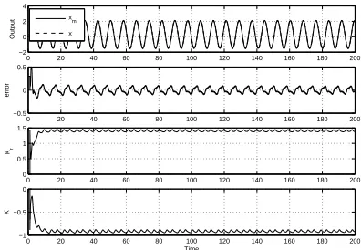
Fig. 10 shows the control result by following the design process. In this case the system is stable and robust, related examples are discussed by [4, 5].
6
Conclusions
In this paper we have introduced a robust design process for a scalar model reference adaptive control (MRAC) algorithm. Different types of MRAC control rules have been reviewed and analysed in the frequency domain by using Bode plot analysis. Then a design process for MRAC has been developed for systems with plant settling times in the range 0.01-100 seconds which is relevant to a wide range of mechanical systems. By using this design method a robust adaptive window is obtained meaning
0 20 40 60 80 100 120 140 160 180 200
−2 0 2 4
Output
0 20 40 60 80 100 120 140 160 180 200
−0.5 0 0.5
error
0 20 40 60 80 100 120 140 160 180 200
0 0.5 1 1.5
Kr
0 20 40 60 80 100 120 140 160 180 200
−1 −0.5 0
Time
K
x
m
x
Figure 10: Plant with unmodelled high frequency dynam-ics, damping ratio 0.1, controlled byρ φmodified MRAC. Input signal r(t)=0.3+1.85sin(0.8t), α = β = 9.85,
ρ2 = 0.5, φ2 = 5. System is unstable, and error and gains settle within around 10 seconds.
that the system is robust in the presence of noise or un-modelled dynamics. An example of applying this method to hydraulic shaking table model with unmodelled oil col-umn resonance is given to demonstrate the usefulness of the design process.
Acknowledgements
Lin Yang would like to acknowledge the support of the Dorothy Hodgkin Postgraduate Award scheme. David Wagg would like to acknowledge the support of EPSRC Advanced Research Fellowship.
References
[1] Karl J. Astr¨om and Bj¨orn Wittenmark. Adaptive control.
Addison-Wesley, second edition, 1995.
[2] Y. D. Landau. Adaptive control:The model reference
ap-proach. Marcel Dekker:New York, 1979.
[3] S. Sastry and M. Bodson. Adaptive control:Stability,
con-vergence and robustness. Prentice-Hall:New Jersey, 1989. [4] L. Yang, S.A. Neild, and D.J. Wagg. Modified model ref-erence adaptive control for plants with unmodelled high
frequency dynamics. InICINCO Int Conf Informatics in
Control, Automation & Robotics, pages 196 – 201, Angers, France., May 2007.
[5] L. Yang, S.A. Neild, D.J. Wagg, and D.W. Virden. Model reference adaptive control of a nonsmooth dynamical sys-tem. Nonlinear Dynamics, 46(3):323–335, 2006.
[6] H. K. Khalil. Nonlinear Systems. Macmillan:New York,
1992.
[7] D. P. Stoten and M. Di Bernardo. Application of the minimal control synthesis algorithm to the control and
synchronization of chaotic systems. International Journal
of Control, 65(6):925–938, 1996.