Proceedings of the 2011 Conference on Empirical Methods in Natural Language Processing, pages 1128–1136,
Efficient Subsampling for Training Complex Language Models
Puyang Xu
[email protected] Asela Gunawardana #
[email protected] [email protected] Khudanpur
Department of Electrical and Computer Engineering Center for Language and Speech Processing
Johns Hopkins University Baltimore, MD 21218, USA
#Microsoft Research Redmond, WA 98052, USA
Abstract
We propose an efficient way to train maximum entropy language models (MELM) and neural network language models (NNLM). The ad-vantage of the proposed method comes from a more robust and efficient subsampling tech-nique. The original multi-class language mod-eling problem is transformed into a set of bi-nary problems where each bibi-nary classifier predicts whether or not a particular word will occur. We show that the binarized model is as powerful as the standard model and allows us to aggressively subsample negative training examples without sacrificing predictive per-formance. Empirical results show that we can train MELM and NNLM at1% ∼ 5%of the
standard complexity with no loss in perfor-mance.
1 Introduction
Language models (LM) assign probabilities to se-quences of words. They are widely used in many natural language processing applications. The prob-ability of a sequence can be modeled as a product of local probabilities, as shown in (1), wherewi is the ithword, andhiis the word history precedingwi.
P(w1, w2, ..., wl) = l
Y
i=1
P(wi|hi) (1)
Therefore the task of language modeling reduces to estimating a set of conditional distributions
{P(w|h)}. The n-gram LM is a dominant way to parametrizeP(w|h), where it is assumed thatwonly depends on the previousn−1words. More complex
models have also been proposed–MELM (Rosen-feld, 1996) and NNLM (Bengio et al., 2003) are two examples.
Modeling P(w|h) can be seen as a multi-class classification problem. Given the history, we have to choose a word in the vocabulary, which can eas-ily be a few hundred thousand words in size. For complex models such as MELM and NNLM, this poses a computational challenge for learning, be-cause the resulting objective functions are expensive to normalize. In contrast,n-gram LMs do not suf-fer from this computational challenge. In the web era, language modelers have access to virtually un-limited amounts of data, while the computing power available to process this data is limited. Therefore, despite the demonstrated effectiveness of complex LMs, then-gram is still the predominant approach for most real world applications.
Subsampling is a simple solution to get around the constraint of computing resources. For the pur-pose of language modeling, it amounts to taking only part of the text corpus to train the LM. For complex models such as NNLM, it has been shown that subsampling can speed up training greatly, at the cost of some degradation in predictive perfor-mance (Schwenk, 2007), allowing for trade-off be-tween computational cost and LM quality.
the vocabulary, we train V binary classifiers, each one of which performs a one-against-all classifica-tion. TheV trained binary probabilities are then re-normalized to obtain a valid distribution over theV words. Subsampling here can be done in the nega-tiveexamples. Since the majority of training exam-ples are negative for each of the binary classifiers, we can achieve substantial computational saving by only keeping subsets of them. We will show that the binarized LM is as powerful as its multi-class coun-terpart, while being able to sustain much more ag-gressive subsampling. For certain types of LMs such as MELM, there are more benefits–the binarization leads to a set of completely independent classifiers to train, which allows easy parallelization and sig-nificantly lowers the memory requirement.
Similar one-against-all approaches are often used in the machine learning community, especially by SVM (support vector machine) practitioners to solve multi-class problems (Rifkin and Klautau, 2004; Allwein et al., 2000). The goal of this paper is to show that a similar technique can also be used for language modeling and that it enables us to sub-sample data much more efficiently. We show that the proposed approach is useful when the dominant modeling constraint is computing power as opposed to training data.
The rest of the paper is organized as follows. In section 2, we describe our binarization and subsam-pling techniques for language models with MELM and NNLM as two specific examples. Experimental results are presented in Section 3, followed by dis-cussion in Section 4.
2 Approximating Language Models with Binary Classifiers
Suppose we have an LM that can be written in the form
P(w|h) = Pexpaw(h;θ)
w0expaw0(h;θ), (2) whereaw(h;θ)is a parametrized history representa-tion for wordw.
Given a training corpus of word history pairs with empirical distribution P˜(h, w), the regularized log likelihood of the training set can be written as
L=X
h ˜ P(h)X
w ˜
P(w|h) logP(w|h)−r(θ), (3)
wherer(θ)is the regularizing function over the pa-rameters.
Assuming thatr(θ)can be written as a sum over per-word regularizers, namely r(θ) = Pwrw(θ), we can take the gradient of the log likelihood w.r.tθ to show that the regularized MLE for the LM satis-fies
X
h ˜ P(h)X
w
P(w|h)∇θaw(h;θ)
=X
h,w ˜
P(w, h)∇θaw(h;θ)−
X
w
∇θrw(θ). (4)
For each wordw, we can define a binary classifier that predicts whether the next word iswby
Pb(w|h) =
expaw(h;θ) 1 + expaw(h;θ)
. (5)
The regularized training set log likelihood for all the binary classifiers is given by
Lb =
X
w
X
h ˜ P(h)
˜
P(w|h) logPb(w|h)
+ ˜P( ¯w|h) logPb( ¯w|h)
−X
w
rw(θ), (6)
wherePb( ¯w|h) = 1−Pb(w|h)is the probability of wnot occurring. Here we assume the same structure of the regularizerr(θ).
The regularized MLE for the binary classifiers satisfies
X
h ˜ P(h)X
w
Pb(w|h)∇θaw(h;θ)
=X
h,w ˜
P(w, h)∇θaw(h;θ)−
X
w
∇θrw(θ). (7)
Notice the right hand sides of (4) and (7) are the same. Thus, takingP0(w|h) = Pb(w|h)from ML trained binary classifiers gives an LM that meets the MLE constraints for language models. Therefore, ifPwPb(w|h) = 1, ML training for the language model is equivalent to ML training of the binary classifiers and using the probabilities given by the classifiers as our LM probabilities.
these probabilities have to be normalized explicitly. Our hope is that for large enough data sets and rich enough history representationaw(h;θ), we will get
P
wPb(w|h) ≈ 1 so that renormalizing the classi-fiers to get
P0(w|h) = P Pb(w|h)
w0∈V Pb(w0|h) (8)
will not change the MLE constraint too much.
2.1 Stratified Sampling
We note that iterative estimation of the LM shown in (2) in general requires enumerating over the T training cases in the training set and computing the denominator of (2) for each case at a cost ofO(V). Thus, each iteration of training takesO(V T)in gen-eral. The complexity of estimating each of the V binary classifiers isO(T)per iteration, also giving O(V T)per iteration in total.
However, as mentioned earlier, we are able to maximally subsample negative examples for each classifier. Thus the classifier for w is trained us-ing the C(w) positive examples and a proportion α of the T −C(w) negative examples. The total number of training examples for allV classifiers is then (1−α)T +αV T. For large V, we choose α >> 1+1V so that this is approximately αV T. Thus, our complexity for estimating allV classifiers isO(αV T).
The resulting training set for each binary classi-fier is a stratified sample (Neyman, 1934), and our estimate needs to be calibrated to account for this. Since the training set subsamples negative examples by α, the resulting classifier will have a likelihood ratio
Pb(w|h) 1−Pb(w|h)
= expaw(h;θ) (9)
that is overestimated by a factor of 1
α. This can be corrected by simply adding logα to the bias (uni-gram) weight of the classifier.
2.2 Maximum Entropy LM
MELM is an effective alternative to the standardn -gram LM. It provides a flexible framework to incor-porate different knowledge sources in the form of feature constraints. Specifically, MELM takes the
form of (2), for wordwfollowing historyh, we have the following probability definition,
P(w|h) = exp
P
iθifi(h, w)
P
w0∈V exp
P
iθifi(h, w0)
. (10)
fi is the ith feature function defined over the word-history pair,θiis the feature weight associated withfi. By defining general features, we have a nat-ural framework to go beyond n-grams and capture more complex dependencies that exist in language. Previous research has shown the benefit of including various kinds of syntactic and semantic information into the LM (Khudanpur and Wu, 2000). However, despite providing a promising avenue for language modeling, MELM are computationally expensive to estimate. The bottleneck lies in the denominator of (10).
To estimate θis, gradient based methods can be used. The derivative of the likelihood function L
w.r.tθihas a simple form, namely
∂L
∂θi
=X
k
fi(wk, hk)−
X
k
X
w0∈V
P(w0|h)fi(w0, hk),
(11) wherekis the index of word-history pair in the train-ing corpus. The first term in the derivative is the ob-served feature count in the training corpus, the sec-ond term is the expected feature count according to the model. In order to obtainP(w0|h)in the second term, we need to compute the normalizer, which in-volves a very expensive summation over the entire vocabulary. As described earlier, the complexity for each iteration of training is atO(V T), where T is the size of training corpus.
separately for different parts of the training data and merged together at the end of each iteration. For models with massive parametrizations, this merge step can be expensive due to communication costs.
Obviously, a different way to expedite MELM training is to simply train on less data. We propose a way to do this without incurring a significant loss of modeling power, by reframing the problem in terms of binary classification. As mentioned above, we buildV binary classifiers of the form in (5) to model the distribution over theV words. The binary clas-sifiers use the same features as the MELM of (10), and are given by:
Pb(w|h) =
expPiθifi(h, w) 1 + expPiθifi(h, w)
. (12)
We assume the features are partitioned over the vo-cabulary, so that each feature fi has an associated w such thatfi(h, w0) = 0 for allw0 6= w. There-fore, the corresponding θi affects only the binary classifier for w. This gives an important advan-tage in terms of parallelization–we have a set of bi-nary classifiers with no feature sharing, and can be trained separately on different machines. The par-allelized computations are completely independent and do not require the tedious communication be-tween machines. Memory-wise, since the compu-tations are independent, each word trainer only have to store features that are associated with the word, so the memory requirement for each individual worker is significantly reduced.
2.3 Neural Network LM
[image:4.612.314.541.68.226.2]Neural Network Language Models (NNLM) have gained a lot of interest since their introduction (Ben-gio et al., 2003). While in standard language mod-eling, words are treated as discrete symbols, NNLM map them into a continuous space and learn their representations automatically. It is often believed that NNLM can generalize better to sequences that are not seen in the training data. However, despite having been shown to outperform standardn-gram LM (Schwenk, 2007), NNLM are computationally expensive to train.
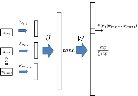
Figure 1 shows the standard feed-forward NNLM architecture. Starting from the left part of the figure, each word of then−1words history is mapped to a
Figure 1: Feed-forward NNLM
continuous vector and concatenated. Through a non-linear hidden layer, the neural network constructs a multinomial distribution at the output layer. Denot-ing the concatenatedd-dimensional word represen-tationsr, we have the following probability defini-tion:
P(wi=k|wi−1, ..., wi−n+1) =
eak P
meam
, (13)
ak=bk+ h
X
l=1
Wkltanh(cl+
(nX−1)d
j=1
Uljrj), (14)
wherehdenotes the hidden layer size, b andcare the bias vectors for the output nodes and hidden nodes respectively. Note that NNLM also has the form of (2).
Stochastic gradient descent is often used to max-imize the training data likelihood under such a model. The gradient can be computed using the back-propagation method. To analyze the complex-ity, computing ann-gram conditional probability re-quires approximately
O((n−1)dh+h+V h+V) (15)
V = 10000, the majority of the complexity per iter-ation comes from the termhV. For large scale tasks, it may be impractical to train an NNLM.
A lot of previous research has focused on speeding up NNLM training. It usually aims at removing the computational dependency on V. Schwenk (2007) used a short list of frequent words such that a large number of out-of-list words are taken care of by a back-off LM. To reduce the gradient computation introduced by the normal-izer, Bengio and Senecal (2008) proposed a dif-ferent kind of importance sampling technique. A recent work (Mikolov et al., 2011) applied Good-man’s class MELM trick (2001) to NNLM, in or-der to avoid the gigantic normalization. A similar technique has been introduced even earlier which took the idea of factorizing output layer to the ex-treme (Morin, 2005) by replacing theV-way predic-tion by a tree-style hierarchical predicpredic-tion. The au-thors show a theoretical complexity reduction from O(V) to(logV), but the technique requires a care-ful clustering which may not be easily attainable in practice.
Subsampling has also been proposed to acceler-ate NNLM training (Schwenk, 2007). The idea is to select random subsets of the training data in each epoch of stochastic gradient descent. After some epochs, it is very likely that all of the training exam-ples have been seen by the model. We will show that our binary classifier representation leads to a more robust and promising subsampling strategy.
As with MELM, we notice that the parameters of (14) can be interpreted as also defining a set of V per-word binary classifiers
Pb(wi =k|wi−1, ..., wi−n+1) = e
ak
1 +eak, (16)
but with a common hidden layer representation. As in MELM, we will train the classifiers, and renor-malize them to obtain an NNLM over theV words.
In order to train the classifiers, we need to com-pute all V output nodes and propagate the errors back. Since the hidden layer is shared, the classifiers are not independent, and the computations can not be easily parallelized to multiple machines. How-ever, subsampling can be done differently for each classifier. Each training instance serves as a positive example for one classifier and as a negative
exam-ple for only a fractionα of the others. The rest of the nodes are not computed and do not produce er-ror signal for the hidden representation. We calibrate the classifiers after subsampled training as described above for MELM.
It is straightforward to show that the dominating termV hin the complexity is reduced to αV h. We want to point out that compared with MELM, sub-sampling the negatives here does not always reduce the complexity proportionally. In cases where the vocabulary is very small, as shown in (15), com-puting the hidden layer can no longer be ignored. Nonetheless, real world applications such as speech recognition, usually involves a vocabulary of consid-erable size, therefore, subsampling in the binary set-ting can still achieve substantial speedup for NNLM.
3 Experimental Results 3.1 MELM
We evaluate the proposed technique on two datasets of different sizes. Our first dataset is obtained from Penn Treebank. Section 00-20 are used for training(972K tokens), section 21-22 are the val-idation set(77K), section 23-24(86K) are the test set. The vocabulary size of the experiment is 10,000. This is one of the standard setups on which many researchers have reported perplexity results on (Mikolov et al., 2011).
The binary MELM is trained using stochastic gradient descent, no explicit regularization is per-formed (Zhang, 2004). The learning rate starts at0.1 and is halved every time the perplexity on the vali-dation set stops decreasing. It usually takes around 20 iterations before no significant improvement can be obtained on the validation set. The training stops at that time.
We compare perplexity with both the standard in-terpolated Kneser-Ney trigram model and the stan-dard MELM. The MELM isL2regularized and
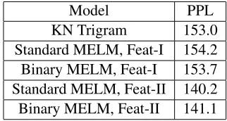
Model PPL KN Trigram 153.0 Standard MELM, Feat-I 154.2 Binary MELM, Feat-I 153.7 Standard MELM, Feat-II 140.2 Binary MELM, Feat-II 141.1
Table 1: Binary MELM vs. Standard MELM
We consider two kinds of feature sets: Feat-I con-tains onlyn-gram features, namely unigram, bigram and trigram features, with no count cutoff, the total number of features is0.9M. Feat-IIis augmented with skip-1 bigrams and skip-1 trigrams (Goodman, 2001), as well as word trigger features as described in (Rosenfeld, 1996). The total number of features in this set is1.9M. Note that the speedup trick de-scribed in (Wu and Khudanpur, 2000) can be used for feat-I, but not feat-II.
Table1shows the perplexity results when no sub-sampling is performed. With onlyn-gram features, the binary MELM is able to match both standard MELM and the Kneser-Ney model. We can also see that by adding features that are known to be able to improve the standard MELM, we can get the same improvement in the binary setting.
Figure 2 shows the comparisons of the two types of MELM when the training data are subsampled. The standard MELM with n-gram features suffers drastically as we sample more aggressively. In con-trast, the binary n-gram MELM(Feat-I) does not appear to be hurt by aggressive subsampling, even when 99%of the negative examples are discarded. The robustness also holds for Feat-II where more complicated features are added into the model. This suggests a very efficient way of training MELM– with only1%of the computational cost, we are able to train an LM as powerful as the standard MELM.
We further test our approach on a second dataset which comes from Wall Street Journal corpus. It contains 26M training tokens and a test set of 22K tokens. We also have a held-out validation set to tune parameters. This set of experiments is intended to demonstrate that the binary subsampling tech-nique is useful on a large text corpus where training a standard MELM is not practical, and gives a better LM than the commonly used Kneser-Ney baseline.
Figure 2: Subsampled Binary MELM vs. Subsampled Standard MELM
Model PPL
[image:6.612.104.265.71.157.2]KN Trigram 117.7 Standard MELM, Trigram 116.5 Binary MELM, Feat-III, 10% 110.2 Binary MELM, Feat-III, 5% 110.8 Binary MELM, Feat-III, 2% 112.1 Binary MELM, Feat-III, 1% 112.4
Table 2: Binary Subsampled MELM on WSJ
The binary MELM is trained in the same way as described in the previous experiment. Besides un-igram, bigram and trigram features, we also added skip-1 bigrams and skip-1 trigrams, this gives us 7.5M features in total. We call this set of features feat-III. We were unable to train a standard MELM with feat-III or a binary MELM without subsam-pling because of the computational cost. However, with our binary subsampling technique, as shown in Table2, we are able to benefit from skipn-gram fea-tures with only5%of the standard MELM complex-ity. Also the performance does not degrade much as we discard more negative examples.
To show that such improvement in perplexity translates into gains in practical applications, we conducted a set of speech recognition experiments. The task is on Wall Street Journal, the LMs are trained on 37M tokens and are used to rescore then -best list generated by the first pass recognizer with a trigram LM. The details of the experimental setup can be found in (Xu et al., 2009). Our baseline LM is an interpolated Kneser-Ney4-gram model.
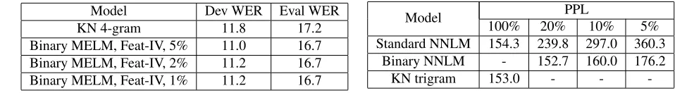
[image:6.612.338.516.264.368.2]Model Dev WER Eval WER
KN 4-gram 11.8 17.2
Binary MELM, Feat-IV, 5% 11.0 16.7
Binary MELM, Feat-IV, 2% 11.2 16.7
[image:7.612.57.536.71.137.2]Binary MELM, Feat-IV, 1% 11.2 16.7
Table 3: WSJ WER improvement. Binary MELM are interpolated with KN 4-gram
is 20K, for the purpose of rescoring, we are only interested in the words that exist in the n-best list, therefore, for the binary MELM, we only have to train about 5300 binary classifiers. For comparison, the KN 4-gram also uses the same restricted vocabu-lary. The features for the binary MELM aren-gram features up to4-grams plus 1 bigrams and skip-1 trigrams. The total number of features is skip-10M. We call this set of features Feat-IV.
Table 3 demonstrates the word error rate(WER) improvement enabled by our binary subsampling technique. Note that we can achieve 0.5% abso-lute WER improvement on the test set at only1% of the standard MELM complexity. More specifi-cally, with only 50 machines, such a reduction in complexity allows us to train a binary MELM with skipn-gram features in less than two hours, which is not possible for the standard MELM on 37M words. Obviously, with more machines, the estimation can be even faster, it’s also reasonable to expect that with more kinds of features, the improvement can be even larger. We think that the proposed technique opens the door for the utilization of the modeling framework provided by MELM at a scale that has not been possible before.
3.2 NNLM
We evaluate our binary subsampling technique on the same Penn Treebank corpus as described for the MELM experiments. Taking random subsets of the training data with the standard model is our primary baseline to compare with. The NNLM we train is a trigram LM with tanhhidden units. The size of word representation and the size of hidden layer are tuned minimally on the validation set(Hidden layer size 200; Representation size 50). We adopt the same learning rate strategy as for training MELM, and the validation set is used to track perplexity per-formance and adjust learning rate correspondingly.
Model 100% 20%PPL10% 5%
Standard NNLM 154.3 239.8 297.0 360.3
Binary NNLM - 152.7 160.0 176.2
KN trigram 153.0 - -
-Table 4: Binary NNLM vs. Standard NNLM. Fixed ran-dom subset.
Model 100% Interpolated PPL20% 10% 5% Standard NNLM 132.7 145.6 148.6 150.7
Binary NNLM - 132.1 134.2 138.0
KN trigram 153.0 - -
-Table 5: Binary NNLM vs. Standard NNLM. Fixed ran-dom subset. Interpolated with KN trigram.
All parameters are initialized randomly with mean0 and variance 0.01. As with binary MELM, binary NNLM are explicitly renormalized to obtain valid perplexities.
In our first experiment, we keep the subsampled data fixed as we did for MELM. For the standard NNLM, it means only a subset of the data is seen by the model and it does not change through epochs; For binary NNLM, it means the subset of negative examples for each binary classifier does not change. Table4shows the perplexity results by NNLM itself and the interpolated results are shown in Table5.
We can see that both models exhibit a tendency to deteriorate as we subsample more aggressively. However, the standard NNLM is clearly impacted more severely. With binary NNLM, we are able to retain all the gain after interpolation with only20% of the negative examples.
Notice that with a fixed random subset, we are not replicating the experiments of Schwenk (Schwenk, 2007) exactly, although it is reasonable to expect both models are able to benefit from seeing different random subsets of the training data. This is verified by results in Table6and Table7.
[image:7.612.317.538.180.245.2]Model 100% 20%PPL10% 5% Standard NNLM 154.3 157.7 172.2 186.5
Binary NNLM - 151.7 150.1 152.1
Table 6: Binary NNLM vs. Standard NNLM. Variable random subset.
Model 100% Interpolate PPL20% 10% 5% Standard NNLM 132.7 133.9 138.1 141.2
[image:8.612.79.296.70.123.2]Binary NNLM - 132.2 131.7 132.2
Table 7: Binary NNLM vs. Standard NNLM. Variable random subset. Interpolated with KN trigram.
4 Discussion
For the standard models, the amount of existent pat-terns fed into training heavily depends on the sub-sampling rateα. For a smallα, the models will in-evitably lose some training patterns given any rea-sonable number of epochs of training. Taking vari-able random subsets in each epoch can alleviate this problem to some extent, but still can not solve the fundamental problem. In the binary setting, we are able to do subsampling differently. While the com-plexity remains the same without subsampling, the majority of the complexity comes from processing negatives examples for each binary classifier. There-fore, we can achieve the same level of speedup as standard subsampling by only subsampling negative examples, and most importantly, it allows us to keep all the existent patterns(positive examples) in the training data. Of course, negative examples are im-portant and even in the binary case, we benefit from including more of them, but since we have so many of them, they might not be as critical as positive ex-amples in determining the distribution.
A similar conclusion can be drawn from Google’s work on large LMs (Brants et al., 2007). Not having to properly smooth the LM, they are still able to ben-efit from large volumes of web text as training data. It is probably more important to have a highn-gram coverage than having a precise distribution.
The explanation here might lead us to wonder whether for the multi-class problem, subsampling the terms in the normalizer would achieve the same results. More specifically, instead of summing over
all words in the vocabulary, we may choose to only considerα of them. In fact, the short-list approach in (Schwenk, 2007) and the adaptive importance sampling in (Bengio and Senecal, 2008) have ex-actly this intuition. However, in the multi-class setup, subsampling like this has to be very careful. We have to either have a good estimate of how much probability mass we’ve thrown away, as in the short-list approach, or have a good estimate of the entire normalizer, as in the importance sampling approach. It is very unlikely that an arbitrary random subsam-pling will not harm the model. Fortunately, in the bi-nary case, the effect of random subsampling is much easier to analyze. We know exactly how much nega-tive examples we’ve discarded, and they can be com-pensated easily in the end.
It is worth pointing out that the proposed tech-nique is not restricted to MELM and NNLM. We have done experiments to binarize the class trick sometimes used for language modeling (Goodman, 2001; Mikolov et al., 2011), and it also proves to be useful. We plan to report these results in the fu-ture. More generally, for many large-scale multi-class problems, binarization and subsampling can be an effective combination to consider.
5 Conclusion
We propose efficient subsampling techniques for training large multi-class classifiers such as maxi-mum entropy language models and neural network language models. The main idea is to replace a multi-way decision by a set of binary decisions. Since most of the training instances in the binary setting are negatives examples, we can achieve sub-stantial speedup by subsampling only the negatives. We show by extensive experiments that this is more robust than subsampling subsets of training data for the original multi-class classifier. The proposed method can be very useful for building large lan-guage models and solving more general multi-class problems.
Acknowledgments
This work is partially supported by National Science Foundation Grant No
References
Allwein, Erin, Robert Schapire, Yoram Singer and Pack Kaelbling. 2000. Reducing Multiclass to Binary: A Unifying Approach for Margin Classifiers. Journal of Machine Learning Research, 1:113-141.
Bengio, Yoshua, Rejean Ducharme and Pascal Vincent 2003. A neural probabilistic language model Journal of Machine Learning research, 3:1137–1155.
Bengio, Yoshua and J. Senecal 2008. Adaptive impor-tance sampling to accelerate training of a neural prob-abilistic language model IEEE Transaction on Neural Network, Apr. 2008.
Berger, Adam, Stephen A. Della Pietra and Vicent J. Della Pietra 1996. A Maximum Entropy approach to Natural Language Processing. Computational Lin-guistics, 1996, 22:39-71.
Brants, Thorsten, Ashok C. Popat, Peng Xu, Frank J. Och and Jeffrey Dean 2007. Large language models in ma-chine translation. In Proceedings of 2007 Conference on Empirical Methods in Natural Language Process-ing, 858–867.
Goodman, Joshua 2001. Classes for Fast Maximum Entropy Training. Proceedings of 2001 IEEE Inter-national Conference on Acoustics, Speech and Signal Processing.
Goodman, Joshua 2001. A bit of Progress in Language Modeling. Computer Speech and Language, 403-434. Khudanpur, Sanjeev and Jun Wu 2000. Maximum En-tropy Techniques for Exploiting Syntactic, Semantic and Collocational Dependencies in Language Model-ing. Computer Speech and Language, 14(4):355-372. Mikolov, Tomas, Stefan Kombrink, Lukas Burget, Jan ”Honza” Cernocky and Sanjeev Khudanpur 2011. Ex-tensions of recurrent neural network language model. Proceedings of 2011 IEEE International Conference on Acoustics, Speech and Signal Processing.
Morin, Frederic 2005. Hierarchical probabilistic neural network language model. AISTATS’05, pp. 246-252. Neyman, Jerzy 1934. On the Two Different Aspects
of the Representative Method: The Method of Strati-fied Sampling and the Method of Purposive Selection. Journal of the Royal Statistical Society, 97(4):558-625.
Rifkin, Ryan and Aldebaro Klautau 2004. In Defense of One-Vs-All Classification. Journal of Machine Learn-ing Research.
Rosenfeld, Roni. 1996. A maximum entropy approach to adaptive statistical language modeling. Computer Speech and Language, 10:187–228.
Schwenk, Holger 2007. Continuous space language model. Computer Speech and Language, 21(3):492-518.
Wu, Jun and Sanjeev Khudanpur. 2000. Efficient train-ing methods for maximum entropy language model-ing. Proceedings of the 6th International Conference on Spoken Language Technologies, pp. 114–117. Xu, Puyang, Damianos Karakos and Sanjeev Khudanpur.
2009. Self-supervised discriminative training of statis-tical language models. Proceedings of 2009 IEEE Au-tomatic Speech Recognition and Understanding Work-shop.