An Improved Affine Scaling Interior Point Algorithm for Linear Programming

https://www.scirp.org/journal/jamp ISSN Online: 2327-4379

ISSN Print: 2327-4352

DOI: 10.4236/jamp.2019.710172 Oct. 30, 2019 2531 Journal of Applied Mathematics and Physics

An Improved Affine-Scaling Interior Point

Algorithm for Linear Programming

Douglas Kwasi Boah, Stephen Boakye Twum

Department of Mathematics, Faculty of Mathematical Sciences, University for Development Studies, Navrongo, Ghana

Abstract

In this paper, an Improved Affine-Scaling Interior Point Algorithm for Linear Programming has been proposed. Computational results of selected practical problems affirming the proposed algorithm have been provided. The proposed algorithm is accurate, faster and therefore reduces the num-ber of iterations required to obtain an optimal solution of a given Linear Programming problem as compared to the already existing Affine-Scaling Interior Point Algorithm. The algorithm can be very useful for development of faster software packages for solving linear programming problems using the interior-point methods.

Keywords

Interior-Point Methods, Affine-Scaling Interior Point Algorithm, Optimal Solution, Linear Programming, Initial Feasible Trial Solution

1. Introduction

The Simplex Method (SM) remained a popular solution method of practical lin-ear programming (LP) problems, until the development of interior point meth-ods. [1] was the pioneer in the field and his Projective Scaling Method was able to compete with the SM as applied to realistic problems. As the name suggests, interior point methods approach an optimal point (which is known to be on the boundary of the feasible set) through a sequence of interior points [2]. Unlike the SM, iterates are calculated not on the boundary, but in the interior of the feasible region. Starting with an initial interior point, the method moves through the interior of the feasible set along an improving direction to another interior point. There, a new improving direction is found, along which a move is made to yet another interior point. This process is repeated, resulting in a sequence of interior points that converge to an optimal boundary point. Many different types

How to cite this paper: Boah, D.K. and Twum, S.B. (2019) An Improved Af-fine-Scaling Interior Point Algorithm for Linear Programming. Journal of Applied Mathematics and Physics, 7, 2531-2536.

https://doi.org/10.4236/jamp.2019.710172

Received: August 5, 2019 Accepted: October 27, 2019 Published: October 30, 2019 Copyright © 2019 by author(s) and Scientific Research Publishing Inc. This work is licensed under the Creative Commons Attribution International License (CC BY 4.0).

http://creativecommons.org/licenses/by/4.0/

DOI: 10.4236/jamp.2019.710172 2532 Journal of Applied Mathematics and Physics of interior-point methods for linear programming have been developed. Most of the methods fall under one of the three main categories: the projective and po-tential reduction method, affine-scaling method and path-following methods

[3]. In this paper, an Improved Affine-Scaling Interior Point Algorithm of LP has been proposed with the view of increasing the efficiency of the original algo-rithm due to [4].

2. Materials and Methods

The Affine-Scaling Interior-Point Algorithm was first introduced by [4]. He subsequently published a convergence analysis in [5]. Dikin’s work went largely unnoticed for many years until [6] [7] [8] and [9] rediscovered it as a simple variant of Karmarkar’s algorithm. Here, the problem is rescaled in order to make the initial point stay some distance away from any boundary constraint and then restrict the step length, so that the next move will not reach the boundary. The algorithm is as follows.

Given an optimization problem in standard form: Optimize T

Z =c x

Subject to Ax=b

0,

x≥

where c, A and b are the cost coefficients, technological coefficients and resource availability respectively, the Affine-Scaling Interior-Point Algorithm is summa-rized in the following steps:

Step 1: Given the initial trial solution,

(

)

x= x x  x set

1 2

3

0 0 0

0 0 0

0 0 0

0 0 0 _n

x

x

D x

x

 

 

 

 

=

 

 

 

 

  

   

 Step 2: Calculate A=AD and c=Dc.

Step 3: Calculate _T

( )

and p

P= −I A AA  − A C =Pc where P is a projection

matrix and Cp is a projected gradient.

Step 4: Identify the negative component of Cp having the largest absolute value, and set v to this absolute value. Then Calculate

1 1

1

p

x C

v

θ       = +

      

 , [1.0]

where 0< <θ 1 [4].

Step 5: Calculate x=Dx as the trial solution for the next iteration starting

from step 1.

DOI: 10.4236/jamp.2019.710172 2533 Journal of Applied Mathematics and Physics terminated) [10].

3. Results and Discussions

The Improved Affine-Scaling Interior-Point Algorithm

In the Affine-scaling interior-point algorithm [4] discussed above, the selected constant, θ _{in Equation 1.0 is required to be such that} 0< <θ 1. Thus,

ac-cording to [4], the possible θ _{values should exclude 0 and 1. The selected} constant, θ _{measures the fraction used of the distance that could be moved} before the feasible region is exited [10]. [5] published convergence analysis of the method using θ _{= 0.5. [11] used} θ _{= 2/3 in their convergence result. [10]} used θ values of 0.5 and 0.9 in their Interactive Operations Research (IOR) software. In this study, an investigation into the consequence of θ value of one (1) on the algorithm has been undertaken. Subsequently, it has been observed that, θ value of one (1) gives the least number of iterations of a given LP prob-lem. The observation has led to an improved Affine-scaling interior-point algo-rithm which is the same the Affine-scaling interior-point algoalgo-rithm [4] but with

θ values now given as 0< ≤θ 1.

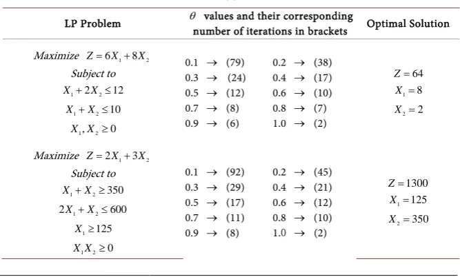
Table 1(a) and Table 1(b) present some computational results of selected practical problems affirming the proposed algorithm. The tables specify the LP problems, selected θ _{values (with their corresponding number of iterations in} brackets) and their optimal solutions using a developed Interior-Point Program based on the Affine-Scaling Interior Point Algorithm which was written in MATLAB. To obtain the optimal solution of any LP problem in standard form, the developed program requires the user to input the initial feasible trial solu-tion (which gives the diagonal matrix), cost coefficients, the number of col-umns/rows of the identity matrix, technological coefficients and the selected constant.

Table 1. (a): Computational results of selected practical problems affirming the proposed algorithm; (b): Computational Results of selected practical problems affirming the pro-posed algorithm.

(a)

LP Problem θ values and their corresponding

number of iterations in brackets Optimal Solution

Maximize Z=6X1+8X2

Subject to

1 2 2 12

X + X ≤

1 2 10

X +X ≤

1, 2 0

X X ≥

0.1 → (79) 0.3 → (24) 0.5 → (12) 0.7 → (8) 0.9 → (6)

0.2 → (38) 0.4 → (17) 0.6 → (10) 0.8 → (7) 1.0 → (2)

64

Z=

1 8

X =

2 2

X =

Maximize Z=2X1+3X2

Subject to

1 2 350

X +X ≥

1 2

2X +X ≤600

1 125

X ≥

1 2 0

X X ≥

0.1 → (92) 0.3 → (29) 0.5 → (17) 0.7 → (11) 0.9 → (8)

0.2 → (45) 0.4 → (21) 0.6 → (12) 0.8 → (10) 1.0 → (2)

1300

Z=

1 125

X =

2 350

DOI: 10.4236/jamp.2019.710172 2534 Journal of Applied Mathematics and Physics Continued

Minimize Z=3X1+2X2

Subject to

1 2

5X +X ≥10

1 2 6 1 4 2 12

X +X ≥ X + X ≥

1 2 0

X X ≥

0.1 → (90) 0.3 → (27) 0.5 → (15) 0.7 → (10) 0.9 → (7)

0.2 → (43) 0.4 → (20) 0.6 → (11) 0.8 → (9) 1.0 → (2)

13 Z= 1 1 X = 2 5 X =

Minimize Z=20X1+10X2

Subject to

1 2 2 40

X + X ≤

1 2 30

3X +X ≥

1 3 2 60

4X + X ≥ 1 2 0

X X ≥

0.1 → (90) 0.3 → (27) 0.5 → (15) 0.7 → (10) 0.9 → (7)

0.2 → (43) 0.4 → (20) 0.6 → (11) 0.8 → (9) 1.0 → (2)

240 Z= 1 6 X = 2 12 X =

Maximize Z=16X1+17X2+10X3

Subject to

1 2 4 3 2000

X +X + X ≤

1 2 3 3600

2X +X +X ≤

1 2 2 2 3 2400

X + X + X ≤

1 30

X ≤

1, 2, 3 0

X X X ≥

0.1 → (122) 0.3 → (37) 0.5 → (19) 0.7 → (12) 0.9 → (10)

0.2 → (58) 0.4 → (26) 0.6 → (15) 0.8 → (11) 1.0 → (3)

20625 Z= 1 30 X = 2 1185 X = 3 0 X = (b) LP Problem

θ values and their corresponding number

of iterations in brackets Optimal Solution

Minimize 1 2 3

4 5 1.06 300 0.56 2703.50 4368. 23

X X X

X X

Z= + +

+ +

Subject to

1 0.01 2

1.06X + 5X ≥729824.87

2 0.649 3

0.56X + X ≥1522188.03

3 50

3.00X ≥ 40.16

4

2703.50X ≥162210.06

5

4368.23X ≥17472. 29

1, 2, 3, 4, 5 0

X X X X X ≥

0.1 → (130) 0.3 → (42) 0.5 → (22) 0.7 → (15) 0.9 → (13)

0.2 → (62) 0.4 → (29) 0.6 → (16) 0.8 → (14) 1.0 → (5)

2435620.485 Z= 1 688490.254 X = 2 2716245.849 X = 3 1680.053 X = 4 60.000 X = 5 4.000 X =

Minimize 1 2 3

4 5 2.03 2.93 0.56 1543.85 1494. 14

X X X

X X

Z= + +

+ +

Subject to

1 3

2.03X +0.015X ≥3604.90

2 3

0.56X + 0.633X ≥430264.03

3

2.93X ≥750.50

4

1543.85X ≥26245. 93

5

1494.14X ≥5976.56

1, 2, 3, 4, 5 0

X X X X X ≥

0.1 → (130) 0.3 → (42) 0.5 → (22) 0.7 → (15) 0.9 → (13)

0.2 → (62) 0.4 → (29) 0.6 → (16) 0.8 → (14) 1.0 → (5)

466675.399 Z= 1 1773.920 X = 2 768039.091 X = 3 256.143 X = 4 17.000 X = 5 4.000 X =

algo-DOI: 10.4236/jamp.2019.710172 2535 Journal of Applied Mathematics and Physics rithm.

4. Conclusion

An Improved Affine-Scaling Interior Point Algorithm for Linear Programming has been proposed. Computational results of selected practical problems affirm-ing the proposed algorithm have been provided. The proposed algorithm is ac-curate, faster and therefore reduces the number of iterations required to obtain an optimal solution of a given Linear Programming (LP) problem as compared to the already existing Affine-Scaling Interior Point Algorithm. The algorithm can be very useful for development of faster software packages for solving linear programming problems using the interior-point methods.

Future Work

In this paper, computational results of selected practical problems affirming the proposed algorithm have been provided. We hope to provide a rigorous proof of the algorithm in the near future.

Conflicts of Interest

The authors declare no conflicts of interest regarding the publication of this paper.

References

[1] Karmarkar, N. (1984) Polynomial-Time Algorithm for Linear Programming.

Com-binatorica, 4, 373-395. https://doi.org/10.1145/800057.808695

[2] Eiselt, H.A. and Sandblom, C.L. (2007) Linear Programming and Its Applications. Springer-Verlag, Berlin Heidelberg, 280.

[3] Singh, J.N. and Singh, D. (2002) Interior-Point Methods for Linear Programming: A Review. International Journal of Mathematical Education in Science and Technol-ogy, 33, 405-423. https://doi.org/10.1080/00207390110119934

[4] Dikin, I.I. (1967) Iterative Solution of Problems of Linear and Quadratic Program-ming. Soviet Mathematics Doklady, 8, 674-675.

[5] Dikin, I.I. (1974) On the Speed of an Iterative Process. Upravlyaemye Sistemi, 12, 54-60.

[6] Karmarkar, N. and Ramakrishnan, U. (1985) Further Developments in the New Polynomial-Time Algorithm for Linear Programming. Talk Given at ORSA/TIMS National Meeting, Boston.

[7] Barnes, E.R. (1986) A Variation on Karmarkar’s Algorithm for Solving Linear Pro-gramming Problems. Mathematical Programming, 36, 174-182.

https://doi.org/10.1007/BF02592024

[8] Vanderbei, R.J., Meketon, M.S. and Freedman, B.A. (1986) A Modification of Kar-markar’s Linear Programming Algorithm. Algorithmica, 1, 395-407.

https://doi.org/10.1007/BF01840454

DOI: 10.4236/jamp.2019.710172 2536 Journal of Applied Mathematics and Physics 297-335. https://doi.org/10.1007/BF01587095

[10] Hillier, F.S. and Lieberman, G.J. (2010) Introduction to Operations Research. Ninth Edition, McGraw-Hill Higher Education, New York, 195-259.

[11] Tsuchiya, T. and Muramatsu, M. (1995) Global Convergence of a Long-Step Affine Scaling Algorithm for Degenerate Linear Programming Problems. SIAM Journal on