ISSN Online: 2327-4379 ISSN Print: 2327-4352
DOI: 10.4236/jamp.2019.710173 Oct. 31, 2019 2537 Journal of Applied Mathematics and Physics
Feature Selection with Non Linear PCA: A
Neural Network Approach
Crescenzio Gallo, Vito Capozzi
Department of Clinical and Experimental Medicine, Foggia, Italy
Abstract
Machine learning consists in the creation and development of algorithms that allow a machine to learn itself, gradually improving its behavior over time. This learning is more effective, the more representative is the features of the dataset used to describe the problem. An important objective is therefore the correct selection (and, possibly, reduction of the number) of the most rele-vant features, which is typically carried out through dimensional reduction tools such as Principal Component Analysis (PCA), which is not linear in the more general case. In this work, an approach to the calculation of the reduced space of the PCA is proposed through the definition and implementation of appropriate models of artificial neural network, which allows to obtain an accurate and at the same time flexible reduction of the dimensionality of the problem.
Keywords
Feature Selection, Machine Learning, Principal Component Analysis, Artificial Neural Network
1. Introduction
The term machine learning [1] refers to one of the fundamental areas of artificial intelligence, centred on the development of systems and algorithms capable of synthesizing a series of subsequent observations. Starting from more or less wide sets of data, the machine—using the themes and algorithms developed—becomes able to automatically recognize complex models and take “decisions”.
Today machine learning technologies [2] are easily accessible (see e.g. Google’s TensorFlow [3] or Microsoft’s Cognitive Services [4][5]) for high-level processing with an emphasis on data semantics. These platforms are proposed as “open’’ tools, accessible by any developer who wants to use artificial intelligence
How to cite this paper: Gallo, C. and Capozzi, V. (2019) Feature Selection with Non Linear PCA: A Neural Network Ap-proach. Journal of Applied Mathematics and Physics, 7, 2537-2554.
https://doi.org/10.4236/jamp.2019.710173
Received: September 16, 2019 Accepted: October 28, 2019 Published: October 31, 2019
Copyright © 2019 by author(s) and Scientific Research Publishing Inc. This work is licensed under the Creative Commons Attribution International License (CC BY 4.0).
http://creativecommons.org/licenses/by/4.0/
DOI:10.4236/jamp.2019.710173 2538 Journal of Applied Mathematics and Physics
to perform complex elaborations and analyze large databases from a machine learning perspective.
When it comes to machine learning, you don’t necessarily have to think about robotics, driving independently or the games DeepMind won [6]: these auto-matic learning systems can also be used to combat spam (by better recognising unsolicited e-mails), to detect intrusion attempts into a computer network, to improve optical character recognition (OCR) skills, and for artificial vision. Search engines themselves make extensive use of them to offer users even more relevant results by analyzing the meaning (semantics) of the query.
The effective use of machine learning techniques depends strongly on the correct modelling of the problem by the researcher, who must be able to capture the fundamental characteristics that allow an effective implementation of the predictive model. If the selected features are excessive with respect to the availa-ble cases, the “power’’ [7] of the corresponding statistical model is compromised, being typically necessary a number of cases in exponential ratio with respect to the number of features of the model.
Therefore, it is of fundamental importance to reduce the number of features, obviously without losing the model’s informative capacity too much. This reduc-tion is usually made through the use of mathematical techniques to reduce the size of the problem such as the Principal Component Analysis (PCA) [8] or the Multi Dimensional Scaling (MDS) [9], which transform the initial data space into a new space with a reduced number of components (the so-called principal Components) on which the original variables are projected.
In this paper an approach to feature reduction by non-linear PCA is presented, this being the most general case. In our approach, the determination of the re-duced space of components is done by setting up appropriate artificial neural network models, of hierarchical or symmetrical type, so as to arrive at the calcu-lation of the main components through the progressive self-learning typical of a neural network.
In the following sections, the general principles of artificial neural networks and PCA are briefly discussed; then the method of calculating PCA through ap-propriate neural network models is presented, and the results are discussed, as well as the conclusions and future directions of research.
2. Artificial Neural Networks for Supervised Learning
Learning by example plays a fundamental role in the process of understanding by humans (in newborns for example, learning is done by imitation, rehearsal and error): the learner learns on the basis of specific cases, not general theories. In essence, learning from examples is a process of reasoning that leads to the identification of general rules based on observations of specific cases (inductive inference).
expli-DOI: 10.4236/jamp.2019.710173 2539 Journal of Applied Mathematics and Physics
cit examples, therefore requires less memory capacity; second, the knowledge learnt contains more information than the examples observed (being a generali-zation is applicable also to cases never observed). In inductive inference, howev-er, starting from a set of true or false facts, we arrive at the formulation of a gen-eral rule that is not necessarily always correct: in fact, only one false assertion is sufficient to exclude a rule. An inductive system therefore offers the possibility of automatically generating knowledge that can be false. The frequency of errors depends strongly on how the set of examples on which the system is to be learned was chosen and how representative this is of the universe of possible cases.
Artificial neural networks (ANNs) [10] [11] are, among the tools capable of learning from examples, those with the greatest capacity for generalization, be-cause they can easily manage situations not foreseen during the learning phase. These are computational models that are directly inspired by brain function and are at an advanced stage of research. An artificial neural network can be thought of as a machine designed to replicate the principles with which the neurons of the human brain work. In the field of automatic learning, a neural network is a mathematical-informational model called upon to solve engineering problems in different fields of application. This allows the creation of an adaptive system that changes its structure based on the flow of external or internal information that flows through the network during the learning phase.
Neural networks are non-linear structures that can be used to simulate com-plex relationships between inputs and outputs that other analytical functions cannot represent. The external signals are processed and processed by a set of input notes, in turn connected with multiple internal nodes (organized into le-vels): each node processes the signals received and transmits the result to the following nodes. Since neural networks are trained using data, connections be-tween neurons are strengthened and output gradually forms patterns, which are well-defined patterns that can be used by the machine to make decisions.
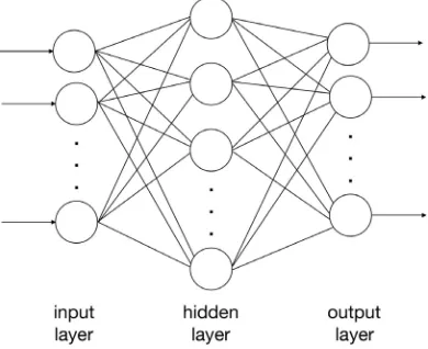
Largely abandoned during the winter of artificial intelligence, neural networks are now at the centre of most projects focused on artificial intelligence and ma-chine learning in particular [2]. They consist of a layer of input neurons (ele-mentary computational units), a layer of output neurons and possibly one or more intermediate layers called hidden (see Figure 1). Interconnections range from one layer to the next and the signal values can be both discrete and conti-nuous. The weight values associated with the input of each node can be static or dynamic in such a way as to plastically adapt the behaviour of the network ac-cording to the variations of the input signals.
DOI:10.4236/jamp.2019.710173 2540 Journal of Applied Mathematics and Physics Figure 1. An example of artificial neural network.
As for the realizations, even if the networks have an autonomous structure, generally computer simulations are used in order to allow even substantial mod-ifications in a short time and with limited costs. However, the first neural chips [12] are being created that have a performance considerably higher than that of a simulation but that has so far had very little diffusion due mainly to high costs and extreme structural rigidity.
3. Application of Neural Networks for Pattern Classification
Pattern recognition is currently the area of greatest use of neural networks. It consists in the classification of objects of the most varied nature in classes de-fined a priori or automatically created by the application based on the similari-ties between the objects in input (in this case we speak of clustering).To perform classification tasks through a computer, real objects must be represented in numerical form and this is done by performing, in an appropriate way, a modeling of reality that associates each object with a pattern (vector of numerical attributes) that identifies it. This first phase is called feature extraction [13], so you can think of reducing them in order to speed up the classification process. This can be done manually or with automatic techniques such as Multi Dimensional Scaling [9] or Principal Component Analysis [8] (see next Section), resulting in a pattern shift to a new space with features that can be classified more simply. After this further phase—which is called preprocessing—we finally move on to the construction of the classifier, which can be seen as a black box capable of associating each input pattern to a specific class.
Suppose, more formally, that you need to classify a pattern p=
(
p1,,pn)
in a class belonging to the set C={
c1,,ck}
. Against the p input pattern, the classifier will output the binary vector z=(
z1,,zk)
where zi =1 if the pat-tern belongs to the class ci, otherwise 0.representa-DOI: 10.4236/jamp.2019.710173 2541 Journal of Applied Mathematics and Physics
tive sample of patterns, and then make the same network work on the set of all possible patterns. At this point we distinguish two different types of learning: supervised and unsupervised.
In “supervised learning’’, the set of patterns on which the network must learn (training set) is accompanied by a set of labels that show the correct classifica-tion of each pattern. In this way, the network makes a regulaclassifica-tion of its structure and internal parameters (connection weights and thresholds) until it obtains a correct classification of training patterns. Given the above mentioned generali-zation capabilities, the network will work correctly even on external patterns and independent from the training set, provided that the training set itself is suffi-ciently representative.
In “unsupervised learning’’, a set of labels cannot be associated with the train-ing set. This can happen for various reasons: the correspondtrain-ing classes can be simply unknown and not obtainable manually or only inaccurately or slowly or, again, the a-priori knowledge could be ambiguous (the same pattern could be labeled differently by different experts). In this type of learning, the network tries to organize the patterns of the training set into subgroups called clusters [14] using appropriate similarity (or distance) measures, so that all the objects longing to the same cluster are as similar (near) as possible while the objects be-longing to different clusters are as different (distant) as possible. Next, you need to use the expert’s a-priori knowledge to label the clusters obtained in the pre-vious step in order to make the classifier usable.
These two different approaches to learning give rise to the different types of neural networks [15] which are used in this work for the implementation of the non-linear PCA calculation algorithm.
4. Principal Component Analysis
Rarely are the characteristics obtained during the extraction phase used as input for a classification, but often some transformation is necessary to facilitate the pattern classification. One of the most frequent problems to solve is the decrease of the pattern dimensionality (of the number of characteristics) in order to make the machine learning algorithms functioning more efficient and faster.
DOI:10.4236/jamp.2019.710173 2542 Journal of Applied Mathematics and Physics
network with greater capacity for generalization. The problem now is to choose, among the characteristics we have available, those to be preserved and those to be discarded, trying to lose as little information as possible. The PCA helps us in this.
Principal Component Analysis is a statistical technique whose aim is to reduce the size of patterns and is based on the selection of the most significant characte-ristics, that is those that bring more information. It is used in many fields and under different names: Karhunen-Loeve expansion, Hotelling transformation, approach to signal subspace, etc.
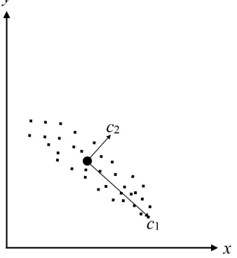
Given a statistical distribution of data in an L-dimensional space, this tech-nique examines the properties of distribution and tries to determine the compo-nents that maximize variance or, alternatively, minimize the misrepresentation. These components are called “main components’’ and are linear combinations of random variables with the property of maximizing the variance in relation to the eigenvalues (and therefore the eigenvectors) of the covariance matrix of the distribution. For example, the first main component is a linear normalized com-bination that has maximum variance, the second main component has second maximum variance and so on. Geometrically, the PCA corresponds to a rotation of the coordinated axes in a new coordinate system such that the projection of the points on the first axis has maximum variance, the projection on the second axis has second maximum variance and so on (see Figure 2). Thanks to this important property, this technique allows us to reduce a space of features, pre-serving as much as possible the relevant information.
Mathematically, the PCA is defined as follows. Consider an M-dimensional vector p obtained from some distribution centered around the average
( )
0E p = and define X =E pp
( )
T the distribution’s covariance matrix. Thei-th main component of p is defined as T
i
v p, where v represents the normalized
[image:6.595.290.459.522.706.2]eigenvector of X corresponding to the i-th largest eigenvalue λ. The subspace obtained by the eigenvectors v1,,vL with L<M , is called the PCA subspace
DOI: 10.4236/jamp.2019.710173 2543 Journal of Applied Mathematics and Physics
of size L. We will then examine the mathematical and neural methods to com-pute the principal components of a distribution.
5. Computation of the Principal Components
Consider N points in an M-dimensional space (which could be a space of fea-tures) by indicating each of them with
[
]
T1, , , 1, ,
i i iM
p = p p i= N and
sup-pose, without loss of generality, that E p
( )
i =0. We can represent the generic vector pi as a linear combination of a set of M vectors in this way:1 M
i ij j
j
p a v
=
=
∑
(1)where the aij are coefficients such that E a
( )
ij =0 when varying by i, whilej
v are orthonormal vectors (v viT j=δij) such that T
1, , , 1, ,
j j jM
v =v v j= M. If we define ai =
[
ai1,,aiM]
T,i=1,,N then Equation (1) can be expressed in matrix form as: pi= ⋅V ai where v is the column matrix of the vj vectors. In this case the explicit expression for the vectors ai is:T
i i
a =v p.
Suppose you want to reduce the size of the space from M to L with L<M in
order to lose as little information as possible. The first step is to rewrite equation (1) this way:
1 1
L M
i ij j ij j
j j L
p a v a v
= = +
=
∑
+∑
(2)to then replace all aij (for j= +L 1,,M ) with constant kj so that each ini-tial pi vector can be approximated by a new pi vector so defined:
1 1
L M
i ij j j j
j j L
p a v k v
= = +
=
∑
+∑
(3)In this way we get a size reduction, since the second sum is constant and therefore each M-dimensional vector pi can be expressed in an approximate way using an L-dimensional vector ai. Let’s now see how to find the base vec-tors vj and the coefficients kj to minimize the loss of information. The error on pi obtained from the size reduction is given by:
(
)
1 M
i i ij j j
j L
p p a k v
= +
− =
∑
− ⋅ (4)We can then define a EL function that calculates the sum of the squares of the errors as follows:
(
)
22
1 1 1
1 1
2 2
N N M
L i ij j
i i j L
E p p a k
= = = +
=
∑
− =∑ ∑
− (5)where we used the relation of “orthonormality’’. If we put the derivative before
L
E compared to kj equal to zero, we get that:
1 1 0 N j ij i k a N =
=
∑
= (6)DOI:10.4236/jamp.2019.710173 2544 Journal of Applied Mathematics and Physics
function can then be rewritten as:
2 T T T
1 1 1 1 1
1 1 1
2 2 2
M N M N M
L ij j i i j j j
j L i j L i j L
E a v p p v v Xv
= + = = + = = +
= = =
∑ ∑
∑
∑
∑
(7)where the first step follows from the fact that T ij j i
a =v p and X is the covariance
matrix of the distribution so defined:
( )
(
)
(
( )
)
T(
T)
1 1
N N
i i i i i i
i i
X p E p p E p p p
= =
=
∑
− − =∑
(8)having set E p
( )
i =0. Now you just have to minimize the EL function com-pared to the choice of base vectors vj.The best choice is when the base vectors meet the condition: Xvj =λjvj for constants λj corresponding to the eigenvectors of the matrix X. It should also be noted that, since the covariance matrix is real and symmetrical, its eigenvec-tors can be chosen orthonormal as required. Returning to the analysis of the er-ror function, we notice that:
1 1 2 M L i i L E λ = +
=
∑
(9)so the minimum error is obtained by discarding the smaller M−L
eigenva-lues and their corresponding autovectors, and keeping the larger L that norma-lized will build the V matrix. The procedure for calculating the principal com-ponents is shown in Figure 3.
6. Neural Implementation of Standard PCA
The Principal Component Analysis can also be carried out through a neural network in which the weight vectors of the neurons converge, during the learn-ing phase, to the main eigenvectors vj
(
j=1,,L)
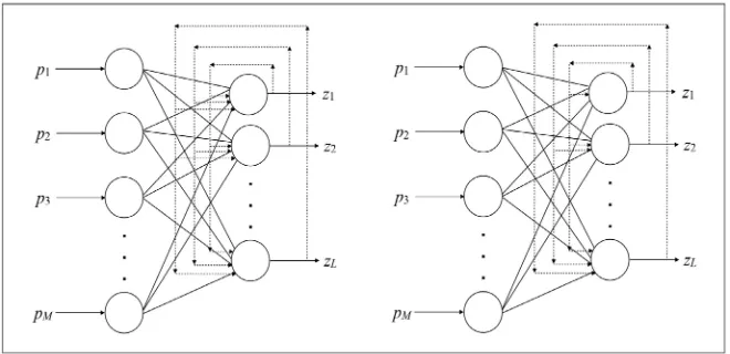
. Such networks have alearning of Hebbian type: the value of a synaptic connection in input to a neuron is increased if and only if the input and the output of the neuron are simulta-neously active. They are composed of a layer of M input neurons designed to perform the sole task of passing the inputs to the next layer, and a layer of L output neurons totally connected to the previous one. The weights of each out-put neuron form an M-dimensional weight vector representing an eigenvector. Feedback connections exist during learning: if the output of the generic neuron reaches all output neurons indiscriminately as input, we are in front of a sym-metrical network; if instead there is an order of neurons according to which each neuron sends its output to itself and to neurons with higher indexes we are in front of a hierarchical network (see Figure 4). After the learning phase these connections (dashed in the Figure) are removed and the network becomes pure-ly feedforward.
This network carries out Hebbian learning (therefore unsupervised). The synaptic modification law, however, is not the standard Hebbian rule:
( )t1 ( )t ( )t ( )t
j j j
DOI: 10.4236/jamp.2019.710173 2545 Journal of Applied Mathematics and Physics Figure 3. Identifying the principal components.
Figure 4. Symmetrical PCA network (left) and hierarchical PCA network (right).
where ( )t
p , ( )t
w and z( )t are, respectively, the value of j-th input, j-th weight
and the output of the network at time t (the network is supposed to be composed of a single neuron), while η is the learning rate. Direct application of this rule would still make the network unstable. Oja [16] proposed another type of rule for changing weights over time, which turns the network into a principal com-ponent analyzer. He thought of normalizing the weight vectors at every step and, starting from (10), he obtained the following equation:
( )t 1 ( )t ( )t ( )t ( ) ( )t t
j j j j
w + =w + ⋅η z ⋅p −z w (11)
where ( )t ( )t j
z p
η⋅ ⋅ is the usual Hebbian increase, while ( ) ( )t t j
z w
− is the stabi-lizing term that makes the sum of the
( )
( )
21 L
t j j
w
=
∑
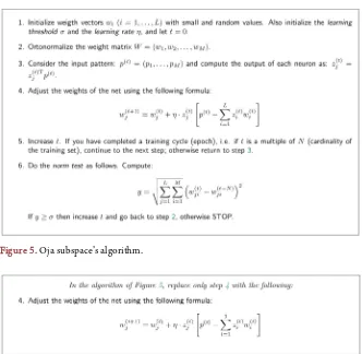
(12)limited and close to 1 without explicit normalisation appearing. The Oja rule can be generalized for networks that have multiple output neurons by obtaining the two algorithms in Figure 5 and Figure 6. The first uses a symmetrical network and the second a hierarchical network. In both algorithms the weight vectors must be orthonormalized or: T
W W =I .
The PCA emerges as an excellent solution to several problems of information representation including:
[image:9.595.208.538.196.356.2]DOI:10.4236/jamp.2019.710173 2546 Journal of Applied Mathematics and Physics Figure 5. Oja subspace’s algorithm.
Figure 6.Sange’s algorithm (Generalized hebbian algoritm).
Minimization of quadratic mean error when the input data is approximated using a linear subspace of smaller size;
Non correlation of outputs after an orthonormal transformation; Minimization of entropy of representation;
At the same time, the PCA network has some limitations that make it less at-tractive;
The network is able to carry out only linear input-output correspondences; Eigenvectors can be calculated much more efficiently using mathematical
techniques;
The principal components take into consideration only the data covariances that completely characterize only Gaussian distributions;
The network is not able to separate independent subsignals from their linear combinations.
DOI: 10.4236/jamp.2019.710173 2547 Journal of Applied Mathematics and Physics
must be mutually orthonormal). In these algorithms, non-linearity appears only at certain points. In non-linear PCA algorithms, however, all neuron outputs are a nonlinear function of the response. It is also interesting to note that, while the standard PCA to obtain the main components needs some form of hierarchy to differentiate the output neurons (the symmetric algorithm obtains only linear combinations of the main components), in the non-linear generalizations the hierarchy is not so important, since the nonlinear function breaks the symmetry during the learning phase [17].
6.1. Generalization of Variance Maximization
The standard quadratic problem leading to a PCA solution can also be achieved by maximizing output variances T T T T
i i i i i i
E z z =E w pp w =w Xw of a linear
network under orthonality constraints. This problem is not well defined until the M-dimensional weight vectors of the neurons are bound in some way. In the ab-sence of a priori knowledge, orthogonality constraints are the most natural be-cause they allow the measurement of variances along directions that differ in a maximum way from each other.
If we refer to Hierarchical Networks, the i-th weight vector wi is bound to have unitary norm and be orthogonal to vectors wj
(
j=1,,i−1)
. Mathemati-cally, this can be expressed as follows: Ti j ij
w w =δ for j≤i. The optimum
vector wi will then be the i-th principal eigenvector vi of the covariance ma-trix X and the outputs of the PCA network become the principal components of the data vectors. The same problem can be solved with symmetrical networks by adopting the following constraint: T
i j ij
w w =δ for j?i. In matrix form you
have T
W W =I where W =
[
w1,,wL]
and I is the unit matrix. If we now consider the z output of the linear PCA network, the problem can be expressed in compact form as maximization of:( )
2(
T)
tr
E z = W XW (13)
The best solution in this casen is any orthonormal basis of the PCA subspace. It is therefore not unique. The problem of maximizing variance under symme-trical orthonality constraints therefore leads to symmesymme-trical networks, the so-called PCA subspace networks.
Let us now consider the generalization of the problem of maximizing variance for robust PCA. Instead of using the previously defined root mean square, we can maximize a more general average as follows:
(
T)
i
E c p w (14)
The c t
( )
function must be a valid cost function that grows slower than thesquare, at least for large values of t. In particular we hypothesize that c t
( )
isequal, not negative, almost everywhere it continues, differentiable and that
( )
22
c t ≤t for big values of t. In addition its only minimum is reached for
0
t= and c t
( )
1 ≤c t( )
2 if t1 ≤ t2 . Valid cost functions are: ln cosh(
( )
θt)
,( )
2
DOI:10.4236/jamp.2019.710173 2548 Journal of Applied Mathematics and Physics
within which the input values vary. In that case the criterion to maximize, for each weight vector wi, is:
( )
(
T)
( ) T1
l i
i i tj i j ij
j
G w E c p w λ w w δ
=
= +
∑
− (15)In the summation, the Lagrange λ coefficients impose the necessary ortho-normality constraints.
Both the hierarchical and the symmetrical problem can be discussed under the general G criterion. In the symmetrical standard case the upper limit of the summation index is l i
( )
=L; in the hierarchical case it is l i( )
=i. The optimalweight vector of the i-th neuron then defines the robust component of the i-th principal eigenvector vi. The gradient of G w
( )
i relative to wi is:( )
( )
(
T)
( )1,
2
l i i
i ii i ij j
j j i
i
G w
d i E pe x w w w
w λ = ≠λ
∂
= = + +
∂
∑
(16)where e t
( )
is the derivative ∂c t( )
∂t of c t( )
. At optimum the gradientmust be zero for i=1,,L. In addition, Lagrange coefficients’ differentiation
leads to orthonality constraints T i j ij
w w =δ .
A gradient descent algorithm to maximize Equation (14) is obtained by en-tering the d i
( )
estimation of the gradient vector (Equation (16)) at the step ofthe weight update, which becomes:
( )t 1 ( )t ( )t
( )
i i
w + =w + ⋅η d i (17)
To obtain estimates of the standard instantaneous gradient, the average values are simply omitted and the instantaneous values of the quantities in question are used instead. The update then becomes:
( )1 ( ) ( ) ( ) ( )T ( ) ( )T ( )
1 l i
t t t t t t t
i i j j i
j
w + w η I w w p f p w
=
= + ⋅ − ⋅ ⋅
∑
(18)Reconsidering the cost function, the assumptions made about it imply that its derivative f t
( )
is a non-decreasing odd function of t. For stability reasons, itis required to be at least f t
( )
≤0 for t<0 or f t( )
≤0 for t>0. If we de-fine the instantaneous representation error vector as:( ) ( ) ( )
(
( )T ( ))
( ) ( ) ( ) ( ) ( )1 1
l i l i
t t t t t t t t
i j j j j
j j
e p p w w p z w
= =
= −
∑
⋅ = −∑
(19)we can summarize the step of weight updating (Equation (18)) as in Figure 7 Please note that since in the symmetrical case e ki
( )
is the same for all neurons,Equation (18) can also be expressed in matrix form as:
( )t 1 ( )t
(
( ) ( )t tT)
(
T ( )t)
( )t ( )t( )
( )tTW + =W + ⋅ −η I W W ⋅ ⋅p f p W =W + ⋅η e ⋅f z (20)
It is interesting to note that the optimal solution for the robust criterion in general does not coincide with the standard solution but is very close to it. For example if we consider c t
( )
= t , the wi directions that maximizeT i
E p w
are, for some arbitrary non-symmetrical distribution, different from the directions that maximize the
(
)
2T
i
E p w
DOI: 10.4236/jamp.2019.710173 2549 Journal of Applied Mathematics and Physics Figure 7. Robust PCA algorithm for generalization of variance maximization.
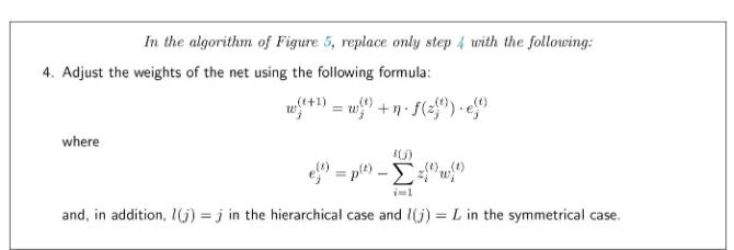
6.2. Generalization of Error Minimization
Let’s consider the linear approximation p of the vectors p in terms of a set of
vectors wj for j=1,,l i
( )
. Since the l i( )
number of base vectors wj is usually smaller than the M size of the data vectors, there will be some error said instantaneous error of representation ( )t ( )t ( )ti i i
e = p −p for each vector p( )t . The
standard PCA solutions are obtained by minimizing the square of this error, namely the quantity: 2 2
i i i
E e =E p −p . Now let’s see how to carry out
the robust generalization of the quadratic mean representation error. Robust PCA algorithms can be achieved by minimizing the criterion:
( )
T( )
1
i i
G e = E c e (21)
where the M-dimensional vector 1 and c t
( )
meet the above mentionedas-sumptions. By minimizing (21) against w we obtain the gradient descent algo-rithm shown in Figure 8. The algorithm can be applied, as usual, both to the symmetrical and hierarchical case; but in the symmetrical case it is l i
( )
=Land therefore:
( )t 1 ( )t
(
( )t( )
( )tT ( )t( )
( )t ( )tT ( )t)
W + =W + ⋅η p ⋅f e ⋅W + f e ⋅p ⋅W (22)
The first term ( )tT
( )
( )t ( )t jw ⋅f e ⋅p in the equation of Figure 8 is proportional
to p for all weight vectors. In addition we can assume that the average value of the coefficient ( )tT
( )
( )tj
w ⋅f e is close to zero because the error vector ( )t
e must
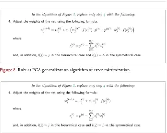
be relatively small after an initial convergence. This term can therefore be over-looked without making a big mistake, which leads us to the algorithm in Figure 9.
Comparing the algorithms of Figure 9 (robust approximate generalization of error minimization) and Figure 7 (robust generalization of variance optimiza-tion) we notice that they, although derived from two different optimization cri-teria, are very similar. The only difference that is noticeable is that the non-linear f t
( )
function is applied to the e( )t error in the first case and the( )t
z output in the second. This has an important consequence: if the network
learns through the algorithm of Figure 9, the final input-output match will still be linear; if the algorithm of Figure 7 is used, this does not happen, since the outputs of the network are non-linear:
(
( )tT ( )t)
i
DOI:10.4236/jamp.2019.710173 2550 Journal of Applied Mathematics and Physics Figure 8. Robust PCA generalization algorithm of error minimization.
Figure 9. Robust PCA approximate algorithm of generalization of error minimization.
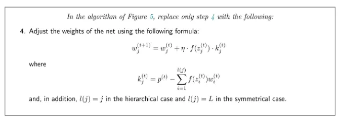
7. Nonlinear PCA
Now let’s consider the non-linear version of PCA. One heuristic way of doing this is to require that neuron outputs are always non-linear and that they are:
( )
( )
Ti i
f z = f w p . Applying this to the equation in Figure 7 we arrive at the
fol-lowing rule of weight adaptation:
( )t 1 ( )t
( )
( )t ( )tj j j j
w + =w + ⋅η f z ⋅k (23)
which is similar to the previous one except that now the error vector is defined as:
( ) ( ) ( )
( )
( ) ( )1
l j
t t t t
j i i
i
k p f z w
=
= −
∑
(24)All this is summarised in Figure 10. In the symmetrical case the algorithm derives directly from the generalization of the algorithm of Oja’s PCA subspace and can be expressed in matrix form as:
( )t 1 ( )t ( )t
( )
( )tTW + =W + ⋅η k ⋅f z (25)
The biggest advantage of this network seems to be the fact that non-linear coefficients implicitly take into account statistical information of degree higher than two, and outputs become more independent than standard PCA networks.
8. Comparison Analysis between Standard and Nonlinear
PCA
DOI: 10.4236/jamp.2019.710173 2551 Journal of Applied Mathematics and Physics Figure 10. Nonlinear PCA algorithm.
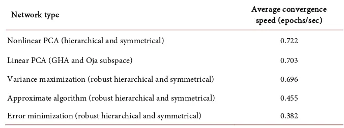
Different types of images from Wolfram Mathematica’s public image reposi-tory CIFAR-1001 were selected for performance testing. After fixing some
sig-nificant parts on each of these, we ran the PCA algorithms of the previous sec-tions to get the main components. The average convergence speed performance for a training set of 10000 images and a learning threshold of 0.00001 is shown
in Table 1. As we can see, the fastest converging networks were the nonlinear
PCA, followed by the linear PCA (GHA and Oja subspace) and, immediately af-ter, the PCA obtained by the generalization of the maximization of the variance.
In order to choose the most effective method, PCA networks have been di-vided into two main classes: networks with linear input-output matching and networks with non-linear input-output matching. The networks of the first type (linear) identify in the images only very bright objects and/or with a clearly dis-tinct outline, confusing the weakest objects with the background. The networks of the second type allow, instead, under certain conditions, to identify also less defined objects. The condition to obtain this result is the use, in the algorithms
of Figure 7 and Figure 10, of an activation function of sigmoidal type
(hyper-bolic tangent) [11]: this type of net gives a greater relief to the pixels of the weak objects detaching them from the background.
9. Discussion and Conclusions
The aim of this paper is to construct an algorithm capable of implementing both standard (linear) and non-linear Principal Component Analysis (PCA) through the use of artificial neural network models. PCA is mainly used to reduce the size (number of features) of a problem but, in the traditional approach, the de-termination of the main components most representative of the phenomenon has the following limitations:
1) The computation is of algebraic (matrix) nature and, for a high number of variables, can involve a high processing time;
2) The standard PCA is suitable for problems with linear relationships be-tween variables.
The approach presented is an algorithm for calculating the principal compo-nents for both standard and non-linear problems. The algorithm makes use of
DOI:10.4236/jamp.2019.710173 2552 Journal of Applied Mathematics and Physics Table 1. Comparison between the standard (linear) and nonlinear PCA.
Network type Average convergence
speed (epochs/sec)
Nonlinear PCA (hierarchical and symmetrical) 0.722
Linear PCA (GHA and Oja subspace) 0.703
Variance maximization (robust hierarchical and symmetrical) 0.696
Approximate algorithm (robust hierarchical and symmetrical) 0.455
Error minimization (robust hierarchical and symmetrical) 0.382
artificial neural network models, with an iterative processing given by the “con-vergence’’ of the network towards the optimal weights, which correspond to the final solution of the problem. The neural network models proposed in the algo-rithm make use of multiple layers of neurons (see Section 6) with the application of the hyperbolic tangent function to the PCA output.
The performance of the proposed approach has been evaluated in a test im-plementation, and can be further improved both in the definition phase of the neural network architecture (number of hidden layers and neurons) and in the learning and validation phase (e.g. through the introduction of cross-validation or leave-one-out depending on the size of the input dataset).
The scaled conjugate gradient learning algorithm leads to a rapidly decreasing average error, up to a level of stabilization. Newton’s method has much slower iterations but, on the other hand, is able to reach values lower than the average error. You can then think of hybridizing the two algorithms using the first one until the average error drops to then exploit the second one starting from the fi-nal weight configuration of the first one. This will lower the error function without wasting too much time.
The performance of the proposed approach, while very good, can be further improved at both the detection and classification stages:
In order to improve the percentage of correctness of the recognition, it is de-sirable to create an algorithm capable of automatically recognising and eli-minating only spurious objects present on a plate;
In order to speed up the learning of the supervised networks for the classification it is possible to think of a hybrid training that exploits the po-tentialities of more algorithms in contemporary.
low-DOI: 10.4236/jamp.2019.710173 2553 Journal of Applied Mathematics and Physics
er on the error function without an excessive loss of time.
Conflicts of Interest
The authors declare no conflicts of interest regarding the publication of this paper.
References
[1] Bishop, C. (2007) Pattern Recognition and Machine Learning (Information Science
and Statistics). Springer, New York.
[2] Schmidt, A. (2016) Cloud-Based AI for Pervasive Applications. IEEE Pervasive
Computing, 15, 14-18.https://doi.org/10.1109/MPRV.2016.11
[3] Abadi, M., Barham, P., Chen, J., Chen, Z., Davis, A., Dean, J., Devin, M., Ghemawat,
S., Irving, G., Isard, M., et al. (2016) Tensor Flow: A System for Large-Scale
Ma-chine Learning. Proceedings of the 12th USENIX Conference on Operating Systems
Design and Implementation, Vol. 16, 265-283.
[4] Del Sole, A. (2018) Introducing Microsoft Cognitive Services. In: Microsoft
Com-puter Vision APIs Distilled, Springer, Berlin, 1-4.
https://doi.org/10.1007/978-1-4842-3342-9_1
[5] Project Oxford—Microsoft Cognitive Services.
https://azure.microsoft.com/en-us/try/cognitive-services
[6] Gregor, K., Besse, F., Rezende, D.J., Danihelka, I. and Wierstra, D. (2016) Towards
Conceptual Compression. Advances in Neural Information Processing Systems, 16,
265-283.
[7] Kraemer, H.C. and Blasey, C. (2015) How Many Subjects? Statistical Power Analysis
in Research. Sage Publications, Thousand Oaks.
https://doi.org/10.4135/9781483398761
[8] Abdi, H. and Williams, L.J. (2010) Principal Component Analysis. Wiley
Interdis-ciplinary Reviews: Computational Statistics, 2, 433-459.
https://doi.org/10.1002/wics.101
[9] Borg, I. and Groenen, P.J.F. (2005) Modern Multidimensional Scaling: Theory and
Applications. Springer Science & Business Media, Berlin.
[10] Demuth, H.B., Beale, M.H., De Jess, O. and Hagan, M.T. (2014) Neural Network
Design. Martin Hagan, Oklahoma State University, Stillwater.
[11] Gallo, C. (2015) Artificial Neural Networks Tutorial. In: Encyclopedia of
Informa-tion Science and Technology, Third Edition, IGI Global, Hershey, 6369-6378.
https://doi.org/10.4018/978-1-4666-5888-2.ch626
[12] Maass, W. (2016) Energy-Efficient Neural Network Chips Approach Human
Recogni-tion Capabilities. Proceedings of the National Academy of Sciences, 113, 11387-11389.
https://doi.org/10.1073/pnas.1614109113
[13] Kuo, B.-C. and Landgrebe, D.A. (2004) Nonparametric Weighted Feature
Extrac-tion for ClassificaExtrac-tion. IEEE Transactions on Geoscience and Remote Sensing, 42,
1096-1105.https://doi.org/10.1109/TGRS.2004.825578
[14] Everitt, B. (1977) Cluster Analysis Social Science Research Council. Heinemann
Educational Books, London.
[15] Beale, R. and Jackson, T. (1990) Neural Computing: An Introduction. CRC Press,
DOI:10.4236/jamp.2019.710173 2554 Journal of Applied Mathematics and Physics
[16] Oja, E. (1991) Learning in Nonlinear Constrained Hebbian Networks. Artificial
Neural Networks. Elsevier Science Publishers, Amsterdam.
[17] Schmidhuber, J. (2015) Deep Learning in Neural Networks: An Overview. Neural