Magneto static modeling of the mixed plasma Beta solar atmosphere based on SUNRISE/IMaX data

MAGNETO-STATIC MODELING OF THE MIXED PLASMA BETA SOLAR ATMOSPHERE

BASED ON SUNRISE

/

IMaX DATA

T. Wiegelmann1, T. Neukirch2, D. H. Nickeler3, S. K. Solanki1,4, V. Martínez Pillet5, and J. M. Borrero6

1

Max-Planck-Institut für Sonnensystemforschung, Justus-von-Liebig-Weg 3, D-37077 Göttingen, Germany;[email protected] 2

School of Mathematics and Statistics, University of St. Andrews, St. Andrews KY16 9SS, UK 3

Astronomical Institute, AV CR, Fricova 298, 25165 Ondrejov, Czech Republic 4

School of Space Research, Kyung Hee University, Yongin, Gyeonggi, 446-701, Korea 5

National Solar Observatory, Sunspot, NM 88349, USA 6

Kiepenheuer-Institut für Sonnenphysik, Schöneckstrasse 6, D-79104 Freiburg, Germany Received 2015 July 28; accepted 2015 October 23; published 2015 December 2

ABSTRACT

Our aim is to model the three-dimensional magneticfield structure of the upper solar atmosphere, including regions of non-negligible plasma beta. We use high-resolution photospheric magneticfield measurements from SUNRISE/ IMaX as the boundary condition for a magneto-static magneticfield model. The high resolution of IMaX allows us to resolve the interface region between the photosphere and corona, but modeling this region is challenging for the following reasons. While the coronal magneticfield is thought to be force-free(the Lorentz force vanishes), this is not the case in the mixed plasma β environment in the photosphere and lower chromosphere. In our model, pressure gradients and gravity forces are self-consistently taken into account and compensate for the non-vanishing Lorentz force. Above a certain height(about 2 Mm)the non-magnetic forces become very weak and consequently the magneticfield becomes almost force-free. Here, we apply a linear approach where the electric current density consists of a superposition of afield-line parallel current and a current perpendicular to the Sunʼs gravityfield. We illustrate the prospects and limitations of this approach and give an outlook for an extension toward a nonlinear model.

Key words:methods: numerical –Sun: chromosphere– Sun: corona– Sun: magneticfields– Sun: photosphere

1. INTRODUCTION

While the corona, at least above active regions, has a low plasma β and is usually modeled by the assumption of a vanishing Lorentz force(see Wiegelmann & Sakurai2012, for an overview of solar force-free fields), this is not true in the lower solar atmosphere (see Wiegelmann et al. 2014, for a recent review on magnetic fields in the solar atmosphere). In the photosphere and lower chromosphere, low- and high-β regions exist side by side and non-magnetic forces have to be taken into account to the lowest order with a magneto-static model where the Lorentz force is compensated for by the gradient of the plasma pressure and the gravity force.

The most accurate measurements of the solar magneticfield are available in the photosphere. In active regions, the full magnetic vector can be measured accurately, e.g., with SDO/

HMI, whereas in quiet Sun regions only the line of sight or verticalfield is available with sufficient accuracy for a reliable extrapolation because in weak-field regions there is too much uncertainty in the transverse field components. (Noise in the Stokes vector translates into an uncertainty in the inferred values for the magneticfield; see Borrero & Kobel2011,2012.) These photospheric measurements are extrapolated into the solar atmosphere under certain model assumptions, here using a magneto-static approach. The vertical resolution of the model scales with the horizontal resolution of the photospheric measurements, e.g., about 1400 km forSOHO/ MDI-magneto-grams and 350 km forSDO/HMI. As the non-force-free layer containing the photosphere and lower chromosphere is rather thin (typically less than 2000 km), one can hardly resolve magnetic structures here for models using SOHO/MDI- or

SDO/HMI-magnetograms as the boundary condition. The high-resolution magnetograms from SUNRISE/IMaX with a

pixel size of only 40 km now allow us to model this layer vertically with about 50 points.

A special class of magneto-static solutions which allow for separable solutions has been proposed by Low (1991). An advantage of this approach is that the resulting equations are linear (for nonlinear cases, see Neukirch 1997) and can be solved effectively by a Fourier transformation or a Greenʼs function implementation(see Petrie & Neukirch2000). Separ-able and linear solutions have also been found in spherical (Bogdan & Low 1986; Neukirch 1995; Al-Salti & Neukirch

2010)as well as cylindrical coordinates (Neukirch 2009; Al-Salti et al.2010). The solutions found in spherical coordinates especially have been used for modeling the global magnetic field of the Sun (e.g., Bagenal & Gibson 1991; Gibson & Bagenal 1995; Gibson et al. 1996; Zhao et al. 2000; Ruan et al.2008)and other stars(e.g., Lanza2008,2009).

provide an outlook for a generalization of the method toward a nonlinear numerical approach.

2. BASIC EQUATIONS

We use the magneto-hydro-static(MHS)equations

j´B=  + YP r , ( )1

B m₀j, ( )2

 ´ =

B 0, 3

· ( )

 =

where Bis the magneticfield, jis the electric current density,

P is the plasma pressure, ρ is the mass density, Ψ is the gravitational potential, andm₀is the permeability of free space. To find separable solutions for this set of equations, we apply the following ansatz for the electric current density (see Low

1991, for details):

B a0B f z( ) Bz ez, ( )4

 ´ = +  ´

wherea0is the force-free parameter and f z( )is a free function

which controls the non-magnetic forces. The first part, a0B, corresponds to afield-line-parallel linear force-free current and the second term, f z( )Bz´ez, defines a current perpendicular

to the gravitational force(in thez-direction)or, in other words, parallel to the Sunʼs surface(x y, ).It is then possible to reduce the MHS equations to a single partial differential equation(see, e.g., Neukirch & Rastätter 1999, for a particularly simple formulation) that can often be solved by the separation of variables. For convenience, here we use (as proposed in Low 1991)

f z( )=aexp(-kz), ( )5

with a free parameterawhich controls the non-magnetic forces in the photosphere. We note thatκin Equation(5)controls the non-magnetic forces and should not be confused with the scale height of the plasma pressure. Obviously, for the choice of

a=0, this approach reduces to linear force-freefields. Above a certain height in the solar atmosphere, one expects that the solution will become approximately force-free due to the low plasma β in the solar corona. Consequently, f z( ) has to decrease with height and here we choose as the scale height the distance of the upper chromosphere above the solar surface, leading to 1 k=2 Mm. With κ fixed, our MHS solution contains two free parameters,αand a.

As boundary conditions we use the measured vertical magnetic fieldB x yz( , , 0)in the photosphere. We solve the equations by means of a Fast-Fourier-Transform method similar to the linear force-free model developed by Alissandrakis (1981). A main difference from the linear force-free approach is that the resulting Schrödinger equation for Bz in Fourier space contains a Bessel function instead of an exponential function.

One finds the following solution for pressure and density (see Low1991, for the derivation):

P P z 1 f z B

2 z, 6

0 0 2 ( ) ( ) ( ) m = -B g dP dz g df dz B f B 1 1

2 . 7

z z 0 0 2 ( · ) ( ) ⎡ ⎣ ⎢ ⎤ ⎦ ⎥ r m = - + + 

Thefirst term in Equation(6)contains a 1D solution(in thez -direction) that is independent of the magneticfield and must

obey = - YP r .The second term is the disturbance of this 1D pressure profile by the magnetic field. Here, the pressure and density compensate for the non-vanishing Lorentz force. This disturbance is negative(ifa >0)and obtains its highest absolute values in regions of the highest vertical magneticfield strength Bz. Because the total plasma pressure (sum of both terms)has to be positive, we obtain the following inequality for

P z0( ):

P z a exp kz Max B z

2 , 8

z 0 2 0

( )

-where MaxB z 2

z2

0

( )

( )

m is the maximum at a given height z. As we

will see later, this condition has severe consequences for an application to data with strong locally enhanced magneticfields in the photosphere. To satisfy condition(8)in these regions, the background pressureP0has to be so high that the plasmaβin

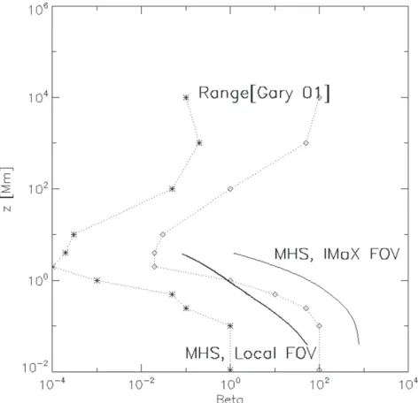
weak-field regions (and also on average) becomes unrealisti-cally high, see Figure 3. Within this limitation, the choice of

P z0( )has some freedom. Our choice is given in Section4.1.

3. DATA

We apply our newly developed code to the photospheric magnetic field measurements taken with the balloon-borne SUNRISE solar observatory in 2009 June. For an overview of the SUNRISE mission and scientific highlights of the first SUNRISEflight see Solanki et al.(2010), Barthol et al.(2011), Berkefeld et al. (2011), and Gandorfer et al. (2011). For a description of the IMaX instrument, we refer to Martínez Pillet et al.(2011). The photospheric magneticfield was computed by inverting the IMaX measurements using the VFISV code as described in Borrero et al. (2011). The linear force-free extrapolation code, and the particular case of an a=0 potentialfield has been applied to data from SUNRISE/IMaX before for a single magnetogram by Wiegelmann et al.(2010)

and to analyze a time series by Wiegelmann et al. (2013). Chitta et al.(2014)carried out nonlinear force-free extrapola-tions from IMaX magnetograms and added vertical flows at low heights to simulate non-force-free effects in the photo-sphere and chromophoto-sphere. Here, we apply our newly developed linear MHS-code to a snapshot of the quiet Sun, also observed with SUNRISE/IMaX. We apply our codefirst to the fullfield of view of IMaX, as shown in Figure 1, and in a subsequent step we investigate a subfield(marked with a black rectangular in Figure1)in more detail. The data set used here was observed in a period of 1.616 hr starting at 00:00 UT on 2009 June 9 (image 220 from this series), see Martínez Pillet et al.(2011).

4. RESULTS

4.1. Application to the Full IMaX-FOV

In our first computation, we apply our model to the full phase-diversity reconstructed IMaX magnetogram of a quiet Sun region of 37×37 Mm, which has been resolved by 936×936 pixels(pixel size on Sun 40 km), see Figure1. As our main interest lies in the mixed plasma β regions of the photosphere and chromosphere, we extrapolate up to a height of z=4 Mm or 100 pixels. A few sample field lines for a magneto-static solution witha=3.0anda=0.5are shown in in Figure1(b).

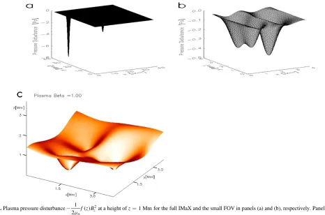
In Figure 2(a), we show the pressure disturbance in the chromosphere at a height ofz=1 Mm as calculated with the second term 1 f z B_z

2

2

0

( )

-m on the right-hand side of Equation(6).

This term obviously becomes largest above those regions with the highest photospheric field strength, as seen in the large negative peaks. Of course, the total pressure has to be positive and consequently a lower bound for the 1D background pressure P0 is given by Equation (8). P0 describes a 1D

equilibrium between the gravity force and the vertical pressure

gradient. One has to solve

dP z

dz g z 9

0( ) _{= - r( ) ( )}

for a constant gravityg. Assuming an equation of state of the formP0=rRT, we get

dP z dz

gP z

RT , 10

0( ) _{= -} 0( ) _{( )}

Figure 1.Panel(a): SUNRISE/IMaX magnetogram of a quiet Sun area. The black rectangular marks the region of interest. Panel(b): Samplefield lines for a MHS-model.

Figure 2.Plasma pressure disturbance 1 f z B

2 ₀ z

2

( ) m

which leads to the well-known atmospheric exponential decay ( exp z ,

H 2

(

)

µ - withH»180 km)for a constant temperature of

T=T0, which is, however, not realistic for describing structures reaching from the photosphere through the chromo-sphere and into the corona. Equation(10)can be(numerically) integrated for any choice of a temperature profileT z( ), e.g., from 1D models of the solar atmosphere. Another alternative (because we already computed the 3D magnetic field from Equations(4)and (5))is to prescribe the average plasmab( )z

as a function of z, e.g., from the literature(Gary2001), leading to

P z z B

2 , 11

0 ave

2

0

( ) b( ) ( )

m

=

where Bave( )z is the horizontally averaged B x y zz( , , ). The

allowed ranges forb( )z are bounded from below, however, by Equation(8). A choice which ensures a total positive pressure is obtained by using Equation (8)directly

P z P z a exp kz Max B z

2 , 12

z 0

2

0

( )

( ) ( ) · ( ) · ( ) ( )

m

= +

-where P z( ) is the (prescribed) minimum value of the total pressure at a given height. For P z( )=0, the total plasma pressure becomes zero at the maximum of Bz and remains positive elsewhere. Taking this into account, we can calculate the full average plasmaβ (including the pressure disturbance) from Equation(6), as shown in Figure3by the rightmost curve labeled MHS, IMaX-FOV in Figure 3. The limitations from Equation(8)and a magnetogram with some high peak values in an otherwise weak-field region cause values of plasmaβwhich are too high and outside the range given by Gary(2001; dotted curves). We have to conclude that the linear MHS model

cannot realistically be applied to the whole FOV of the SUNRISE magnetogram. The reason for this is that through Equation (12) the 1D background pressure, and thereby the maximum pressure in weak-field regions, is coupled with the highest values in the photospheric magnetogram, which is not very realistic.

4.2. Application to a Small Part of the FOV

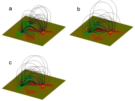
Due to the difficulties involved with applying the linear MHS model to a full magnetogram, we restrict our analysis in the following to the smaller sub-region marked by the black rectangle in Figure 1(a). Figure 4 shows a few sample field lines for (a) a potential field model, (b) a linear force-free model with a=3, and (c) a magneto-static solution

a

3, 0.5.

a= = In the linear force-free case, the field lines become sheared compared with the potential field, and for some lines the connectivity changes. The influence of a non-vanishing Lorentz force(but using the same value ofαas in the linear force-free case) has additional effects, which seem, however, to be smaller. The maximum heights of the loops are somewhat reduced and some additionalfield lines change their connectivity, e.g., in the MHS model no lines are connected with the positive(red)flux region close to the front boundary. Compared with the potential fields, the number offield lines connecting to this region was already reduced in the linear-force-free model.

The pressure disturbance in this smaller FOV is shown in the center panel of Figure 2. The absence of strong peaks in the photospheric field in this region leads to a much smoother distribution of the pressure disturbance. We use Equation(12)

to compute the background pressure, and in Figure3the solid line marked MHS, local FOV shows the averaged plasmaβas a function of the height. At least in the photosphere and chromosphere, the plasmaβ is within the limitation given by the dashed lines from the literature(Gary2001). The true 3D plasmaβdistribution, however, is not a function ofzonly, but varies significantly in the horizontal direction. Figure 2(c) shows the equi-contours for b=1.0. As one can see, the

1.0

b= surface is by no means plane-parallel, but is strongly corrugated. This behavior impacts methods for extrapolating force-free fields. Traditionally and for numerical simplicity, one extrapolates from a plane parallel surface (or the Sunʼs spherical surface)by assuming that the field above this lower boundary of the computational domain is force-free. In reality, however, the force-free domain is also bounded below by a corrugated surface. This is also true for planned measurements of the chromospheric magneticfield vector with Solar-C, and so magnetic field extrapolation techniques bounded by non-plane-parallel surfaces should be developed. In the non-force-free region between the photosphere and the corrugated chromosphere, plasma pressure and gravity must be taken into account.

5. DISCUSSION AND OUTLOOK

The linear MHS approach used in this paper has two free parameters, the linear force-free parameter α and the force parametera. Additionally, one also has to prescribe, in addition to the vertical magneticfield component at the lower boundary, the height in the solar atmosphere where the magnetic field becomes approximately force-free, here1 k=2 Mm. Apply-ing these solutions to large-scale areas has its limitations. These

Figure 3.Plasmaβin the solar atmosphere. The dotted lines are taken from Gary(2001). The thin solid line shows the(horizontally averaged)plasmaβ profile computed with our MHS model for the full IMaX FOV and the thick solid line represents the same for the selected small area.

are,first of all, the well-known limitation ofαbeing constant, which these solutions share with linear force-free confi gura-tions. Additionally, the pressure gradient (which compensates the Lorentz force)is coupled to the vertical magneticfield. As a consequence, the pressure disturbance, which is negative, becomes very large above strongfields in the photosphere. In order to maintain a positive total pressure, the background plasma pressure must be so strong that the average plasma β becomes too high. This limitation of the method has to do with the fact that the two free parameters α and a have to be the same in the entire computational domain. This limitation is similar to that for linear force-free fields, where one has only one free parameterαwhich has to be globally constant. While linear force-free fields cannot be used to model force-free configurations containing strong current concentrations in part of the domain(leading to localized high values ofα), a similar restriction occurs here for the linear magneto-static approach. Strong magnetic elements in an otherwise weak-field magneto-gram cannot be modeled by this class of MHS solutions.

These limitations do not occur, however, for applications to regions with smallerfields of view because the assumption that α and a are constant is naturally more reasonable the smaller the investigated domain is. How should one proceed to derive global magneto-static solutions? One possibility would be to compute the solutions discussed here only locally (with different values of αand a in different regions)and to merge these configurations together. This will, of course, lead to solutions which are not entirely self-consistent and to inconsistencies at the boundaries between the different regions.

Another idea would be to use a numerical scheme, e.g., an optimization approach as suggested by Wiegelmann & Neukirch(2006)and Wiegelmann et al.(2007), to relax these merged solutions toward a self-consistent (nonlinear) MHS-equilibrium. Wiegelmann & Neukirch(2006)and Wiegelmann et al. (2007) developed nonlinear magneto-static codes in Cartesian and spherical geometry, respectively. For the small-scale features measured with SUNRISE, one would naturally apply the cartesian version. These codes require photospheric vector magnetograms as input, which are not available with the required quality for the investigated quiet Sun region because of the poor signal-to-noise ratio(for horizontalfields)in weak-field regions. Nonlinear approaches (both force-free and magneto-static) are well suited to dealing with local strong enhancements (e.g., current concentrations and strong flux elements). It is a weakness of any linear approach that they cannot deal with strong localized enhancements of relevant quantity.

To be able to carry out nonlinear magneto-static (or nonlinear force-free) extrapolations, measurements of the horizontal photospheric magnetic field would be helpful. During the re-flight of SUNRISE in 2013, high-resolution vector magnetograms of active region(s)were measured with IMaX. We plan to use these measurements for self-consistent nonlinear magneto-static modeling in our future work.

The German contribution to SUNRISE is funded by the Bundesministerium für Wirtschaft und Technologie through Deutsches Zentrum für Luft- und Raumfahrt e.V.(DLR), grant

No. 50OU0401, and by the Innovationsfonds of the President of the Max Planck Society (MPG). The Spanish contribution has been funded by the Spanish MICINN under projects ESP2006-13030-C06 and AYA2009-14105-C06 (including European FEDER funds). The HAO contribution was partly funded through NASA grant number NNX08AH38G. T.N. acknowledges support by the U.K.ʼs Science and Technology Facilities Council and would like to thank the MPS for its hospitality during a visit in 2014 December. D.H.N. acknowl-edges financial support from GA ČR under grant number 13-24782S. The Astronomical Institute Ondrejov is supported by̌ the project RVO:67985815. This work was partly supported by the BK21 plus program through the National Research Foundation (NRF) funded by the Ministry of Education of Korea.

REFERENCES

Alissandrakis, C. E. 1981, A&A,100, 197 Al-Salti, N., & Neukirch, T. 2010,A&A,520, A75 Al-Salti, N., Neukirch, T., & Ryan, R. 2010,A&A,514, A38 Bagenal, F., & Gibson, S. 1991,JGR,96, 17663

Barthol, P., Gandorfer, A., Solanki, S. K., et al. 2011, SoPh,268, 1 Berkefeld, T., Schmidt, W., Soltau, D., et al. 2011, SoPh,268, 103 Bogdan, T. J., & Low, B. C. 1986,ApJ,306, 271

Borrero, J. M., & Kobel, P. 2011,A&A,527, A29 Borrero, J. M., & Kobel, P. 2012,A&A,547, A89

Borrero, J. M., Tomczyk, S., Kubo, M., et al. 2011, SoPh,273, 267 Chitta, L. P., Kariyappa, R., van Ballegooijen, A. A., DeLuca, E. E., &

Solanki, S. K. 2014,ApJ,793, 112

Gandorfer, A., Grauf, B., Barthol, P., et al. 2011, SoPh,268, 35 Gary, G. A. 2001, SoPh,203, 71

Gibson, S. E., & Bagenal, F. 1995,JGR,100, 19865

Gibson, S. E., Bagenal, F., & Low, B. C. 1996,JGR,101, 4813 Lanza, A. F. 2008,A&A,487, 1163

Lanza, A. F. 2009,A&A,505, 339 Low, B. C. 1991,ApJ,370, 427

Martínez Pillet, V., Del Toro Iniesta, J. C., Álvarez-Herrero, A., et al. 2011, SoPh,268, 57

Neukirch, T. 1995, A&A,301, 628 Neukirch, T. 1997, A&A,325, 847 Neukirch, T. 2009, GApFD,103, 535

Neukirch, T., & Rastätter, L. 1999, A&A,348, 1000 Petrie, G. J. D., & Neukirch, T. 2000, A&A,356, 735

Ruan, P., Wiegelmann, T., Inhester, B., et al. 2008,A&A,481, 827 Solanki, S. K., Barthol, P., Danilovic, S., et al. 2010,ApJL,723, L127 Wiegelmann, T., & Neukirch, T. 2006,A&A,457, 1053

Wiegelmann, T., Neukirch, T., Ruan, P., & Inhester, B. 2007,A&A,475, 701 Wiegelmann, T., & Sakurai, T. 2012, LRSP,9, 5

Wiegelmann, T., Solanki, S. K., Borrero, J. M., et al. 2010, ApJL, 723, L185

Wiegelmann, T., Solanki, S. K., Borrero, J. M., et al. 2013, SoPh,283, 253 Wiegelmann, T., Thalmann, J. K., & Solanki, S. K. 2014, A&ARv,22, 78 Zhao, X. P., Hoeksema, J. T., & Scherrer, P. H. 2000,ApJ,538, 932