Dust in brown dwarfs and extra solar planets VII Cloud formation in diffusive atmospheres

Astronomy&Astrophysicsmanuscript no. DiffuDrift cESO 2019 November 12, 2019

Dust in brown dwarfs and extra-solar planets

VII. Cloud formation in diffusive atmospheres

Peter Woitke

, Christiane Helling

, and Ophelia Gunn

1 _{Centre for Exoplanet Science, University of St Andrews, St Andrews, UK}

2 _{SUPA, School of Physics & Astronomy, University of St Andrews, St Andrews, KY16 9SS, UK} 3 _{SRON Netherlands Institute for Space Research, Sorbonnelaan 2, 3584 CA Utrecht, NL} 4 _{SUPA, School of Physics and Astronomy, University of Edinburgh, Edinburgh, EH9 3JZ, UK}

Received 10/07/2019; accepted 09/11/2019

ABSTRACT

The precipitation of cloud particles in brown dwarf and exoplanet atmospheres establishes an ongoing downward flux of condensable elements. To understand the efficiency of cloud formation, it is therefore crucial to identify and to quantify the replenishment mech-anism that is able to compensate for these local losses of condensable elements in the upper atmosphere, and to keep the extrasolar weather cycle running. In this paper, we introduce a new cloud formation model by combining the cloud particle moment method of Helling & Woitke with a diffusive mixing approach, taking into account turbulent mixing and gas-kinetic diffusion for both gas and cloud particles. The equations are of diffusion-reaction type and are solved time-dependently for a prescribed 1D atmospheric structure, until the model has relaxed toward a time-independent solution. In comparison to our previous models, the new hot Jupiter model results (Teff≈2000 K, logg=3) show fewer but larger cloud particles which are more concentrated towards the cloud base. The abundances of condensable elements in the gas phase are featured by a steep decline above the cloud base, followed by a shallower, monotonous decrease towards a plateau, the level of which depends on temperature. The chemical composition of the cloud particles also differs significantly from our previous models. Due to the condensation of specific condensates like Mg2SiO4[s] in deeper layers, certain elements, such as Mg, are almost entirely removed from the gas phase early. This leads to unusual (and non-solar) element ratios in higher atmospheric layers, which then favours the formation of SiO[s] and SiO2[s], for example, rather than MgSiO3[s]. Such condensates are not expected in phase-equilibrium models that start from solar abundances. Above the main silicate cloud layer, which is enriched with iron and metal oxides, we find a second cloud layer made of Na2S[s] particles in cooler models (Teff/1400 K).

Key words. planets and satellites: atmospheres – planets and satellites: composition – brown dwarfs – astrochemistry – diffusion

1. Introduction

The number of confirmed extrasolar planets has reached more than 4000, but only a hand-full of them can be studied in detail (see e.g.Nikolov et al. 2016;Huitson et al. 2017;Birkby et al.

2017; Arcangeli et al. 2018). Indirect observations, like

trans-mission spectroscopy, have demonstrated the presence of clouds

(Sing et al. 2016;Nikolov et al. 2016;Pino et al. 2018;Gibson

et al. 2017; Kirk et al. 2018; Tregloan-Reed et al. 2018). Far

easier targets for atmosphere studies are brown dwarfs, which are very similar to planets with respect to their physical param-eters and atmospheric processes. The coolest brown dwarfs (Y dwarfs) reach effective temperatures as low as 250 K (Leggett

et al. 2017; Luhman 2014). The observation of brown dwarfs

allows us to identify the vertical cloud structures (Apai et al.

2013;Buenzli et al. 2015;Yang et al. 2016;Helling & Casewell

2014). To date, between 1500 and 2000 brown dwarfs are known (depending on whether late M-dwarfs and/or early L-dwarfs are included; Gagné et al. 2015; Best et al. 2018) and are rela-tively well-studied compared to the∼4000 extrasolar planets, for which the era of spectral analysis has only just begun.

Cloud formation has a profound impact on the remaining gas phase abundances and radiative transfer effects, but cloud parti-cles will also affect the ionisation state of the atmosphere, which is well known for solar system objects (Helling et al. 2016a,b). Efforts are therefore ongoing to construct physical models

de-scribing the formation of clouds in exoplanet and brown dwarf atmospheres. Such detailed models are necessary tools to pro-vide the context for observations and to uncover processes not directly accessible by observations. Part of this effort is the con-sistent coupling of cloud formation with 1D atmosphere models with radiative transfer and convection (Tsuji et al. 1996;

Acker-man & Marley 2001;Tsuji 2002;Witte et al. 2009;Allard et al.

2012; Juncher et al. 2017; alsoHelling et al. 2008a), but also

in 3D in order to study the time-dependent climate of extrasolar planets (Lee et al. 2016;Lines et al. 2018a) and to understand observational implications beyond 1D (Lee et al. 2017; Lines

et al. 2018a).

As our understanding of cloud formation progresses (e.g.

Lee et al. 2015b;Krasnokutski et al. 2017;Hörst et al. 2019),

including its implication for habitability (Narita et al. 2015), we start to refine our approaches. One long-standing discussion is how to model the element replenishment in 1D cloud forming atmospheres, because without replenishment, a quasi-static at-mosphere must be cloud free (Appendix A inWoitke & Helling

2004).Parmentier et al.(2013) utilised passive tracers to study

the atmospheric mixing in 3D (shallow water approximation) simulations for irradiated, dynamic but convectively stable atmo-spheres of (giant gas) planets. They observe that cloud particles are distributed throughout the whole atmosphere.

Parmentier et al.(2013) state: “In statistical steady state, this

upward dynamical flux balances the downward transport due to

particle settling and allows the atmospheric tracer abundance to equilibrate at finite (non-zero) values despite the effect of par-ticle settling. The mechanism does not require convection, and indeed, the vertical motions that cause the upward transport in our models are resolved, large-scale motions in the stably strat-ified atmosphere. These vertical motions are a key aspect of the global-scale atmospheric circulation driven by the day-night heating contrast.” This assessment confirms our conclusion that the upward transport of condensable elements through the at-mosphere by mixing is indeed the key to understand cloud for-mation. However, challenges arise from the choice of the in-ner boundary condition (Carone et al. 2019), chemical gradi-ents (Tremblin et al. 2019), and the need to include cloud ticle feedback in order to test mixing parameterisations. A par-ticular interesting case will be the ultra-hot Jupiters where day and night-sides can be expected to have very distinct (verti-cal) mixing patterns and scales. In this paper, we consider self-luminous giant gas planets, for which the irradiation from their host stars is negligible, such as young giant gas planets and brown dwarfs. Brown dwarfs atmospheres are by now under-stood to be rather similar to giant gas planets, in particular at-mospheres from low-gravity brown dwarfs and young gas giants

(Charnay et al. 2018).

Moses et al.(2000) point out that large-scale mixing helps

to homogenise a gravitationally stratified atmospheres consist-ing of different kinds of molecules. This, however, only prevails up to a certain altitude above which gas-kinetic diffusion starts to dominate over mixing (Zahnle et al. 2016). Different approaches have been chosen to represent this vertical mixing in 1D atmo-sphere models (Ackerman & Marley 2001;Woitke & Helling

2004;Helling et al. 2008a;Allard 2014;Juncher et al. 2017) and

in 3D models (Lee et al. 2015a;Lines et al. 2018b) by measur-ing vertical velocity fluctuations and derivmeasur-ing mixmeasur-ing parame-terisations from 2D or 3D radiation-hydrodynamics simulations

(Ludwig et al. 2002a;Freytag et al. 2010;Parmentier et al. 2013;

Zhang & Showman 2018).

Cloud formation modelling becomes an increasingly impor-tant part also of exoplanet/brown dwarf retrieval approaches for which, however, computational speed is an essential limitation. As part of the ARCiS1retrieval platform,Ormel & Min(2019) presented a fast forward model that consistently solves diffusive mixing and cloud particle growth for exoplanet atmospheres.

In this paper, we present a new theoretical approach that consistently combines cloud formation modelling with diffusive transport for element replenishment. After presenting the main formula body of our model in Sects.2.1to2.3, we summarise our ansatz for handling the diffusion coefficient in Sect.2.4, be-fore we present our main results in Sects. 4 and 5. We conclude in Sect. 6. An overview of quantifying diffusion coefficients in the literature is provided in AppendixD.

2. Cloud formation with diffusive transport of gas and cloud particles

Cloud formation involves at least seed particle formation (nucle-ation), surface growth and evaporation, element depletion, grav-itational settling and element replenishment. During their decent through the atmosphere, cloud particles may change phase or, more general, chemical composition, and may collide with each others leading to further growth. These cloud formation pro-cesses have been described previously (Woitke & Helling 2003;

Helling & Woitke 2006;Helling & Fomins 2013) and different

1 _{ARtful modelling Code for exoplanet Science}

cloud formation models have been compared byHelling et al.

(2008a) with an update byCharnay et al.(2018). We therefore

only provide a short summary here, a recent review can be found

inHelling(2019).

Clouds are made of particles (aerosols, droplets, solid par-ticles). The formation of these particles requires condensation seeds, which are produced, for the case of the Earth atmosphere, by volcano eruptions, ocean sprays and wild fires. In absence of these crucial processes, which all require the existence of a solid planet surface, cloud formation needs to start with the formation of seed particles through chemical reactions in the gas phase, involving the formation of molecular clusters. The formation of seed particles requires a highly supersaturated gas. Once such seed particles become available, many materials are already ther-mally stable and can condense on these surfaces simultaneously. Nucleation and growth reduce the local element abundances and have a strong feedback on the local composition of the atmo-spheric gas. As macroscopic cloud particles form, they display a spectrum of sizes as well as a mixture of condensed mate-rials. The local particle size distribution and the material mix-ture change as the cloud particles move through the atmosphere (hence, encounter different thermodynamic conditions), for ex-ample by gravitational settling (rain). Particle-particle collision will continue to shape the size distribution function. Cloud par-ticles may break up into smaller units (shattering) or stick to-gether to form even bigger units (coagulation). Cloud particles may also be transported upward and downward by macroscopic mixing processes. Particle-particle processes are not part of our present model which focuses on the formation of cloud parti-cles and their feedback on the local chemistry through element depletion/enrichment. We note that the surface growth does shut offthe nucleation process due to efficient element depletion (Lee

et al. 2015b) such that a simultaneous treatment of nucleation

and growth is required in order to calculate the number of cloud particles forming in the first place.

2.1. Cloud formation as reaction-diffusion system

As introduced inWoitke & Helling(2003), we consider the evo-lution of the size distribution function f(V) [cm−6_{] of cloud}

par-ticles in the particle volume intervalV...V+dVas affected by advection, settling, surface reactions and (new) by diffusion ac-cording to the following master equation

∂ f(V)dV ∂t +∇

v(V)f(V)dV = X

k

RkdV − ∇φddV. (1)

Rk are the various gain and loss rates due to surface chemical reactions, which lead to growth and evaporation of the particles (see Eqs. 59-62 for large Knudsen numbers, and Eqs. 68-71 for small Knudsen numbers inWoitke & Helling 2003). The vol-ume of the particlesVis chosen as size variable to formulate the material deposit by surface reactions in the most straightforward way. The last term in Eq. (1) accounts for the additional gains and losses due to diffusive mixing. The cloud particle velocity v(V) is assumed to be given by the hydrodynamical gas velocity vgasplus a vertical equilibrium drift velocityv

◦ dr(V)

v(V)=vgas+v ◦

dr(V). (2)

Applying Fick’s first law (see e.g. Bringuier 2013), the diff u-sive fluxφdof the cloud particles in volume intervalV...V+dV

gradi-ent of those particles

φddV=−ρDd∇

f(V)dV

ρ !

, (3)

where Dd[cm2s−1] is the diffusion coefficient for those cloud

particles andρ[g/cm3] the gas density. We introduce moments of the cloud particle size distribution as

ρLj= Z ∞

V`

f(V)Vj/3dV. (4)

Multiplying Eq. (1) withVj/3 and integrating over volume, we obtain the following system of moment equations for large Knudsen numbers (see details inWoitke & Helling 2003)

∂(ρLj)

∂t +∇vgasρLj

= _Vj/3 ` J? |{z} nucleation

+ j

3χ ρLj−1 | {z }

growth

− ∇

Z ∞

Vl

vdr(V)f(V)Vj/3dV

| {z } drift

− ∇

Z ∞

Vl

φdVj/3dV

| {z } diffusion

, (5)

where J?[s−1cm−3] is the nucleation rate and χ[cm/s] the net growth velocity. For large Knudsen numbers and subsonic veloc-ities (Epstein regime), the equilibrium drift velocity, also called final fall speed, is given bySchaaf(1963)

v◦_dr=− √

πgρda

2ρcT b

r, (6)

whereais the particle radius,ρdthe cloud particle material

den-sity,_brthe unit vector pointing away from the centre of gravity, andgthe gravitational acceleration.cT=

p

2kT/µ¯ is an abbre-viation,T the temperature,kthe Boltzmann constant, and ¯µthe mean molecular weight of the gas particles.

Using Eq. (6) witha=3₄V_π1/3and assuming that the particle diffusion coefficientDdis independent of size, we can carry out

the integrations in Eq. (5). The final result is ∂(ρLj)

∂t +∇(vgasρLj) =V

j/3 ` J? +

j

3χ ρLj−1

+∇ ξρd

cT

Lj+1br !

+ ∇Ddρ∇Lj

(7)

with abbreviation

ξ=

√

π 2

3 4π

!1/3

g. (8)

A size-dependent diffusion coefficient,Dd(V), would lead to an

open set of moment equations as discussed byHelling & Fomins

(2013).

2.2. Generalisation to mixed materials

We assume that all cloud particles are perfect spheres with well-mixed material composition which is independent of size, but depends on time and location in the atmosphere (Helling &

Woitke 2006;Helling et al. 2008c). Using the indexs =1...S

to distinguish between the different solid materials, for example Al2O3[s], TiO2[s], Mg2SiO4[s] and Fe[s], we write

V=X

s

Vs, L3= X

s

L₃s, J?= X

s

J?s , χ= X

s χs_,

bs=L

s 3

L3 , (9)

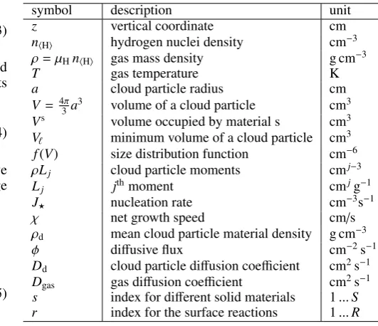
Table 1.Variable definitions and units

symbol description unit

z vertical coordinate cm

nhHi hydrogen nuclei density cm−3

ρ=µHnhHi gas mass density g cm−3

T gas temperature K

a cloud particle radius cm

V= 4π

3a

3 _{volume of a cloud particle cm}3

Vs volume occupied by material s cm3

V` minimum volume of a cloud particle cm3

f(V) size distribution function cm−6

ρLj cloud particle moments cmj−3

Lj jthmoment cmjg−1

J? nucleation rate cm−3s−1

χ net growth speed cm/s

ρd mean cloud particle material density g cm−3

φ diffusive flux cm−2s−1

Dd cloud particle diffusion coefficient cm2s−1

Dgas gas diffusion coefficient cm2s−1

s index for different solid materials 1...S

r index for the surface reactions 1...R

wherebs _{is the volume fraction of material sin the cloud} par-ticles2. The mean cloud particle material density is given by ρd = Psbsρs whereρs is the mass density of a pure material

s. Most materials will not nucleate themselves (J_?s =0), but will use alien nuclei to grow on. Using this approximation, we can split the third moment equation into a set of third moment equa-tions for single materials as follows

∂(ρLs₃)

∂t +∇(vgasρL

s

3) = V`J s

? + χsρL2

+ ∇ξρd

cT

bsL4br !

+∇Ddρ∇L3s

. (10)

Adding up Eqs. (10) for all solidssagain yields Eq. (7) forj=3. The different materials grow at different speeds which depend on the amount of available atoms and molecules in the gas phase and on the supersaturation ratio. Islands of some materials may grow whereas others are thermally unstable and shrink. This be-haviour is obtained by summing up the contributions of all sur-face reactionsr = 1...R (for examples see Table 1 inHelling

et al. 2008c)

χ=X s

χs₌X s

X

r

c_rsV₀s, (11)

whereVs

0[cm

3_{] is the volume of one unit of material of kindsin}

the solid state andcs

r[cm−2s−1] is the effective surface reaction rate

cs_r = 3

√ 36π ν

s rn

key r vrelr αr

νkey r

1− 1

Sr !

×

(

1 if Sr ≥1

bs if Sr <1 , (12)

wherenkeyr is the particle density [cm−3] of the key species of sur-face reactionr,αrthe sticking probability,νkeyr its stoichiometric factor in that reaction, vrel_r = pkT/(2πmkey_{) its thermal relative}

2 _{InHelling et al. (2008c), we have used the notationb}s _{= V} s/Vtot whereVs=ρLs3=

R∞

V` f(V)V

s_{dVis the volume occupied by solidsper}

volume of stellar atmosphere andVtot=ρL3=

R∞

velocity andmkeyits mass. These growth rates are derived from a simple hit-and-stick model where we usually assumeαr=1. The impact of the limited number of known αr ,1 has been studied byHelling & Woitke(2006).Sris the reaction supersat-uration ratio as introduced in (Helling & Woitke 2006, see their App. B). For example, in the reaction

2 CaH + 2 Ti + 6 H2O ←→ 2 CaTiO3[s] + 7 H2 (13)

the key species is either CaH or Ti, depending on which species is less abundant. νkeyr =2 in either case, s=CaTiO3[s] is the

solid species, andνrs=2 units of CaTiO3[s] are produced by one

reaction.

We note that Eq. (12) differs slightly from our previ-ous definition (Eq. 4 in Helling et al. 2008c). The new growth/evaporation rates now always change sign at Sr =1 as they should, independent of the value of bs. When supersatu-rated (Sr>1), we assume that the total surface of the particles acts as a funnel to collect the impinging molecules from the gas phase, followed by fast hopping to find a place on a matching island of kinds(see Fig. 1 inHelling & Woitke 2006). But for under-saturation (Sr<1), we assume that the molecules trigger-ing the evaporation processes must hit one of the islands of the matching kind, the probability of which isbs_.

2.3. Element conservation with diffusive replenishment

An integral part of our cloud formation model is the element con-servation. We must identify a replenishment mechanism which is able to compensate for the losses of elements due to cloud particle formation and settling in the upper atmosphere. In this paper, we include diffusion of gas particles along their concen-tration gradients. As cloud particles form, they consume certain elements in the upper atmosphere, creating a negative element abundance gradient. Thus, gas particles containing those ele-ments will ascent diffusively in that atmosphere. Analogous to the formulation of the master equation for the dust particles, we formulate the element conservation as diffusion-reaction system

∂(nhHik)

∂t +∇(vgasnhHik) = −

X

s νs

kN`J s ? − ρL2

X

s X

r νs

kc s r

+∇DgasnhHi∇k

, (14)

wherekis the abundance of elementkwith respect to hydro-gen. The chemical reactions leading to nucleation and growth appear as negative source terms here, because they consume el-ements. We choose nhHi as density variable in Eq. (14), the

to-tal hydrogen nuclei particle density, which is proportional toρ in hydrogen-dominated atmospheres.nhHikis the total number density [cm−3] of nuclei of elementkin any chemical form.νs k is the stoichiometric factor of elementkin solid s, for example νTiO2[s]

Ti =1, andDgas [cm

2 _s−1_{] is the gas diffusion coefficient.}

For simplicity, we assume that all molecules are transported by the same diffusion coefficient, which is valid within a factor 2 or 3 for gas-kinetic diffusion (sometimes called the binary diff u-sion coefficient, see Eq. (16) and App.D), and is entirely justified when eddy diffusion dominates. The involved diffusive gas ele-ment fluxφ_kdiff[cm−2s−1] is given by

φdiff

k =−DgasnhHi∇k. (15)

2.4. Gas diffusion coefficient

The diffusion coefficients provide the kinetic information to calculate the transport rates from concentration gradients (e.g.

Lamb & Verlinde 2011). In general, gas and cloud particles

dif-fuse with different efficiencies because of their different inertia and collisional cross sections with the surrounding gas.

The determination of the gas diffusion coefficientDgasis of

crucial importance for our model. We include gas-kinetic dif-fusion and large-scale turbulent (eddy) diffusion as mixing pro-cesses. The gas-kinetic diffusion coefficient is given by

Dmicro=

1

3vth` , (16)

where` = 1/(σn) is the mean free path,n the total gas parti-cle density andσ≈2.1×10−15_cm2_{a typical cross-section for}

collisions between the molecules under consideration with H2.

The thermal velocity is defined as vth =

√

8kT/(πmred) where

mredis the reduced mass for collisions between the molecule and

H2(Woitke & Helling 2003). This gas-kinetic diffusion∝1/nis

negligible in the lower high-density layers of brown dwarf and planetary atmospheres, where instead mixing by large-scale tur-bulent or convective motions is the dominant mixing process

(Ackerman & Marley 2001; Ludwig et al. 2002b; Woitke &

Helling 2004; Allard et al. 2012; Parmentier et al. 2013; Lee

et al. 2015a). The large-scale (turbulent/convective/eddy) gas

diffusion coefficient is given by

Dmix≈ hvziL with L=αHp, (17)

wherehvziis the root-mean-square average of the fluctuating part of the vertical velocity in the atmosphere, considering averages over sufficiently large volumes and/or long integration times,L

is the mixing length, andHpis the local pressure scale height.α is a dimensionless parameter of the order of one. We useα=1 in this work, but note that αcan be fine-tuned to describe the actual mixing scales as revealed by detailed hydrodynamic mod-elling. Inside the convective part of the atmospherehvzi ≈vconv

is assumed, where vconv is the convective velocity, which is an

integral part of stellar atmosphere models, derived from mixing length theory in 1D models. Above the convective atmosphere, where the Schwarzschild criterion for convection is false, hvzi decreases rapidly with increasingz, but never quite reaches zero due to convective overshoot (see e.g.Brandenburg 2016). We apply a power-law in logpto approximate this behaviour

loghvzi = log vconv−β0·max n

0,logpconv−logp(z) o

(18)

with a free parameterβ0_{≈0.0...2.2 (Ludwig et al. 2002b). The}

total gas diffusion coefficient is then

Dgas = Dmix+Dmicro. (19)

At high altitudes, the gas densitynis small and henceDmicro is

large, whereas Dmix is small whenβ0>0. Therefore, at some

pressure level in the atmosphere, the gas-kinetic diffusion will start to dominate. Figure1shows a typical structure as assumed in our models. The minimum of Dgasaround 10−3mbar

corre-sponds to the crossover point (called thehomopause), upward of whichDmicrodominates and the atmospheres is not well-mixed.

Moses et al. (2000) draw similar conclusions concerning

Sat-urn’s atmosphere. The maximum ofDgas around pconv=0.2 bar

results from the start of the convective layer, within which both hvzi and Dgas are approximately constant. Appendix D

−8 −7 −6 −5 −4 −3 −2 −1 0 log10 p[bar]

5 6 7 8 9 10 11 12 13

D

[cm

2/s]

−11

−10

−9

−8

−7

−6

−5

−4

1

/τmix

[1

/

s]

D

1/τmix

Fig. 1.The gas diffusion coefficient Dgas (Eq.19) in the new Diffu

-Driftmodel for a brown dwarf atmosphere model withTeff=1800 K,

logg=3 [cm/s2_{] and solar abundances. The grey line shows the inverse} mixing timescaleτmixas assumed in the previous Driftmodel.τmixis calculated according to Eq. (9) in (Woitke & Helling 2004). Both quan-tities are computed forβ=β0₌

1 and bothy-axes show exactly 8 orders of magnitude.

2.5. Cloud particle diffusion coefficient

The diffusion of solid particles due to turbulent gas fluctua-tions was studied, in consideration of protoplanetary discs, by

Dubrulle et al.(1995),Schräpler & Henning(2004),Youdin &

Lithwick (2007) and Riols & Lesur (2018). All works apply

mean field theory (also called Reynolds decomposition ansatz), where the densities and velocities of both the particles and the gas are decomposed into a mean component (that depends only onz) and a small fluctuating part.

The response of the solid particles to the turbulent gas varia-tions is then determined by comparing two timescales. The stop-ping or frictional coupling timescale is given by

τstop =

aρd

vthρ

with vth=

s 8kT

πµ¯ , (20)

whereathe particle radius. Equation (20) follows from a gen-eral relaxation ansatzτstop=m ∂Ffric/∂vdr

_v◦

dr

−1_{, see Eq. (21) in}

Woitke & Helling (2003), for the special case of large

Knud-sen numbers in a subsonic flow (the so-called Epstein regime), which we assume is valid here.

The second timescale is the eddy turnover or turbulence cor-relation timescaleτeddy(l) in consideration of a spectrum of

dif-ferent turbulent modes associated with different wave-numbersk

or different spatial eddy sizesl. In a Kolmogorov type of power spectrumP(k)∝k−5/3, any given cloud particle of sizeatends to co-move with all sufficiently large and slow turbulent eddies whereas its inertia prevents following the short-term, small tur-bulence modes.

In order to arrive at an effective particle diffusion coefficient, the advective effect of all individual turbulent eddies has to be averaged, and thereby transformed into a collective diffusive ef-fect. This procedure is carried out with different procedures and approximations. The result ofSchräpler & Henning(2004, see their Eq. 27), reads

Dd=

Dmix

1+St with St=

τstop τeddy

. (21)

whereDd is the size-dependent cloud particle diffusion coeffi

-cient andStis the Stokes number of the particle in consideration of the largest eddy sizeL. The eddy turnover timescale of the largest turbulence mode is given by

τeddy=

L

hvzi

. (22)

Both the size of the largest eddyLand the average of the fluctu-ating part of the vertical velocityhvziare assumed to be identical to the mixing length and velocity appearing in Eq. (17). Combin-ing the above equations we find

St= aρdDmix

vthρL2

. (23)

The impact of the size dependence of Dd on the cloud

parti-cle moments was explored byHelling & Fomins (2013), who showed that this leads to an open set of moment equations, which seems impractical for an actual solution. In the frame of this work, we will therefore only explore the two limiting cases of very large and very small Stokes numbers throughout the atmo-sphere. For small particles withSt1, we haveDd→Dmixand

for huge particlesSt→ ∞, we haveDd→0.

case 1: Dd=Dmix if all cloud particles are small,

case 2: Dd=0 if all cloud particles are large. (24)

Our results show that both approximations lead to rather similar cloud structures in the models explored so far, i.e. the inclusion of turbulent cloud particle motions does not seem to be a critical ingredient to our present model. However, in preliminary models for hot Jupiters, whereDmix(z) is more flat or even increasing

with height, this might be different.

3. Static plane-parallel atmosphere

Before we proceed with the numerical solution of the full time-dependent model of cloud formation in diffusive media, we first discuss the 1D static case in order to better understand the expected results from these equations. Considering the plane-parallel (∇ →d/dz), static (vgas=0) and stationary case (∂/∂t=

0), our Eqs. (7), (10) and (14) simplify to

0 = V_`j/3J?+ j

3χ ρLj−1+ξ

d dz

ρd

cT

Lj+1 !

+ d

dz Ddρ

dLj

dz

! (25)

0 = V`J_?s +ρL2 X

r

cs_rV₀s+ξd dz

ρd

cT

bsL4 !

+ d

dz Ddρ

dLs 3

dz

! (26)

0 = −X

s νs

kN`J s ?−ρL2

X

s X

r νs

kc s r+

d

dz DgasnhHi

dk

dz

! .(27)

3.1. The total element fluxes

In the hydrostatic stationary case, the total vertical flux of ele-ments (due to vertical settling of cloud particlesand diffusive transport) must be zero everywhere in the atmosphere and for each element. This conclusion can be derived formally by adding together Eq. (27) andP

s(Eq.26)·νks/V s

0, usingV`=N`V s 0. The

exactly, and in caseDd=0 we find

d

dz DgasnhHi

dk

dz

! + ξd

dz        ρd cT L4 X s νs kb s Vs 0        = 0

⇒ DgasnhHi

dk

dz

| {z }

−φ_kdiff

+ ξρd

cT L4 X s νs kb s

V₀s

| {z } φsettle

k

= constk (28)

φdiff k [cm

−2 _s1_{] is the upward element flux by diffusion in the}

gas phase andφsettle

k is the downward flux of elements contained in the settling cloud particles at this point. Equation (28) would still allow for solutions with constant (i.e. time-independent and height-independent) total element fluxes throughout the atmo-sphere, but this would require matching feeding and removing rates at the bottom and the base of the atmosphere, which does not seem to be physically plausible. Thus, constk=0 and we find

φdiff k =φ

settle

k ⇒

dk

dz = −

ξ ρdL4

cTDgasnhHi

X s νs kb s Vs 0

≤ 0. (29)

According to Eq. (29), the element abundance gradients in cloudy, static (vgas =0) and stationary (∂/∂t=0) atmospheres

must be negative because of the downward transport of elements via the precipitation of cloud particles, which must be balanced by an upward directed diffusive flux of elements in the gas phase, which requires a negative concentration gradient. This conclu-sion is correct whenever cloud particles are present (L4>0) and

gravity is active (ξ >0), otherwise the gas element abundances are constant. The abundance gradients of different elements are proportional to the element composition of the settling cloud par-ticles at this point. The abundances of all elementskinvolved in cloud formation must decrease monotonically toward the top of the atmosphere.

4. Numerical solution of the time-dependent cloud formation problem

Equations (25)−(27) form a system of (3+S+K) coupled 2nd

order differential equations, which can be transformed into a system of 2×(3+S+K) 1st _{order ordinary differential}

equa-tions (ODEs). Unfortunately, we have not been able to solve this ODE system directly. The boundary conditions are partly given at the lower and partly at the upper boundary of the model, see Sect.4.4. The integration direction must be downward in order to model the nucleation of new cloud particles. Hence, we tried a shooting method wherek(zmax) is varied at the top of the

at-mosphere untilk(zmin) is met, i.e. the given values in the deep

atmosphere. We found it impossible to proceed this way. A tiny change ofk(zmax) in the 12th digit was still observed to change k(zmin) by a factor of two. The reason for this extreme

sensitiv-ity seems to be the nucleation rate with its threshold character as function of supersaturation, and hence as function ofk.

Looking for alternatives, we found that a simulation of the time-dependent equations on a given vertical grid can be performed by means of the operator splitting method as ex-plained in Sect.4.2. We evolve the atmospheric cloud structure _L

j(z,t),L₃s(z,t), k(z,t) for a sufficiently long time, until it ap-proaches the time-independent case_L◦

j(z),L s,◦

3 (z),

◦

k(z), which is the stationary structure we are interested in. Assuming a plane-parallel (∇ → d/dz) and static (vgas=0) atmosphere, Eqs. (7),

(10) and (14) read, including the time-dependent terms

d dt

ρLj

= V_`j/3J? + j

3χ ρLj−1 (30)

+ ξd

dz

ρd

cT

Lj+1 !

+ d

dz Ddρ

dLj

dz

!

(j=1,2,3)

d dt(ρL

s

3) = V`J s

? + χsρL2 (31)

+ ξd

dz

ρd

cT

bsL4 !

+ d

dz Ddρ

dL₃s dz

!

(s=1...S)

d

dt(nhHik) = −

X

s νs

kN`J s ? − ρL2

X s X r νs kc s r (32) + d

dz DgasnhHi

dk

dz

!

(k=1...K).

4.1. Closure condition

The moment Eqs. (30) and (31) are not closed because L4

ap-pears twice of the right side, a consequence of larger particles settling faster (Eq.6). Therefore, a numerical solution requires a closure condition as

L4=F(L0,L1,L2,L3). (33)

We use the closure condition explained in the appendix A.1 of

(Helling et al. 2008c). The idea is to approximate the particle

size distribution f by a doubleδ-function which has four param-eters. These parameters are determined by matching the given momentsL0,L1,L2 andL3, and result in the forth momentL4

according to the definition of the dust moments (Eq.4).

4.2. Operator splitting method

Figure2 visualises our numerical approach using the operator splitting method (Klein 1995).

1. We update Lj and Ls₃ only according to the settling source terms (the terms on the right side of Eqs. (30) and (31) con-tainingLj+1 andL4), applying half a timestep∆t/2, see

de-tails in App.B.

2. We call the diffusion solver for half a timestep∆t/2 to update kand, optionally,LjandLs₃, if the cloud particles are to be diffused as well, see App.A.

3. We integrate the chemical source terms (nucleation, growth and evaporation) for a full timestep ∆t. These equations are stiffat high densities and require an implicit integration scheme. We use the implicit ODE-solver L_imex4.2A1 (

Deu-flhard & Nowak 1987). The computation of the chemical

source terms on the r.h.s. proceeds as follows: (i) for given temperatureT, densitynhHiand element abundancesk, we

call the equilibrium chemistry code GGchem(Woitke et al.

2018) to calculate all molecular concentrations; (ii) those re-sults are used to calculate the reaction supersaturation ratios

Sr; (iii) the nucleation ratesJ?s and net surface reaction rates

cs

rare determined.

4. We finish the timestep by calling again the diffusion solver for∆t/2 and the settling solver for∆t/2 in this order. 5. Checkpoint and output files are written for visualisation.

1 2Sett

1

2Diff 1 CF

1 2Diff

1

2Sett OP

Fig. 2.Operator splitting calling sequence. Sett=gravitational settling,

Diff =diffusion, CF=cloud formation (nucleation, growth and evapora-tion), and OP=output. 1/2 means half a timestep and 1 a full timestep.

is why we do not split CF (Fig.2) but put it with a full timestep in the centre of the operator splitting calling sequence. The cloud formation part of the code is parallelised and can be executed for all atmospheric layers independent of each other.

4.3. Timestep control

In order to produce accurate 2nd order solutions, the timestep must be limited to make sure that each operator remains in the linear regime. For example, the sole application of a cloud-chemistry timestep must not change the amount of dust or the el-ement abundances substantially in any computational cell. In or-der to achieve code stability and accuracy, we limit the timestep as follows:

1. The cloud particles must not jump over layers by settling

∆t < 0.5 ∆z vdr,j

(34)

where∆zis the vertical grid resolution and vdr,jis the mean

drift velocity affecting moment ρLj as given by Eq. (B.3). This is the usual Courant-Friedrichs-Lewy (CFL) criterion to stabilise explicit advection scheme, with an additional safety-factor 1/2.

2. Nucleation and cloud particle growth and evaporation, as in-tegrated over∆t, must not change any of the gas element abundances by more than a given maximum relative change (default accuracy is 15%).

3. The timestep must not exceed the maximum explicit diff u-sion timestep (Eq.A.27).

If one of these criteria becomes false during the simulation, the timestep is discarded and∆treduced. If, on the contrary, the cri-teria are met easily,∆tis increased for the subsequent timestep.

4.4. Boundary conditions

As our upper boundary condition, we assume that there are no cloud particles settling into the model volume from above vdr,j(zmax)=0. In the diffusion solver, we use a zero-flux (closed

box) upper boundary condition, i.e. the gradients of k are as-sumed to be zero atz=zmax. The same applies to the cloud

parti-cle moments d

dzLj(zmax)=0 if they are to be diffused as well. The lower boundary is placed well below the main silicate cloud layer to make sure that the temperature is too high to allow for any cloud particles to exist near the lower boundary

Lj(zmin)=0. We also demand that the element abundances at

the lower boundary equal the given values as present deep in the atmosphere k(zmin) = _k0, where the _k0 are considered as free

parameters, for example solar abundances (Asplund et al. 2009).

4.5. Initial conditions

We start all simulations from a cloud-free atmosphere Lj(z,t= 0) = 0. Concerning the element abundances, we have experi-mented with two cases: (1) an ‘empty’ atmospherek(z,t=0)=0

or (2) a ‘full’ atmospherek(z,t=0)=_k0, where the index k is applied to all elements which can potentially be transformed completely into solids (k=Si, Mg, Fe, Al, Ti, ...), but not H, He, C, N, O, etc. For the latter elements we putk(z,t=0)=_k0 in both cases. We found an identical final structure in both cases (see App.C), which is very reassuring. The models calculated from initial condition (2), however, need much more computa-tional time to complete. In this case, the nucleation rate is ini-tially huge and a very large number of tiny cloud particles are created shortly after initialisation, which take a long time to set-tle down in the atmosphere.

In order to reach the final relaxed, time-independent state, the model must be evolved until (i) the atmosphere is completely re-plenished several times by fresh elements ascending diffusively from the lower boundary to the very top and (ii) new grains formed high in the atmosphere have sufficient time to settle down to the cloud base and evaporate. In comparison, the chemical processes are typically quite fast. We need to evolve one model for about 106_{timesteps, which, depending on global parameters}

like Teff and logg, translates into real evolutionary times

be-tween a few months to a few tens of years. On a parallel cluster, one can complete one such model in a few days real time when using 16 processors (about 500 CPU hours), where the chemical equilibrium solver GGchemis called a few 109times.

5. Results

5.1. Comparison to our previous cloud formation model

In the previous Helling & Woitke cloud formation models

(Woitke & Helling 2004;Helling & Woitke 2006;Helling et al.

2008c), henceforth called the D_riftmodels, the replenishment of

elements was treated in a different way, using a prescribed mass exchange timescale τmix(z) to replenish the atmosphere with

fresh elements from the deep asnhHi(_k0−k)/τmix. The mass

ex-change timescale was approximated by a powerlaw logτmix(z)=

const−βlogp(z) with power-law indexβ=2.2 to describe con-vectional overshoot, see equation 9 inWoitke & Helling(2004). This simple approach led to an ODE-system which can be solved within about 2 CPU-min.

Figure 3 compares the results of a previous Drift model with the new diffusive model, henceforth called the DiffuDrift model. Both approaches model seed formation, kinetic surface growth/evaporation of cloud particles and gravitational settling in the same way, but differ in the treatment of the mixing which enters the cloud formation and the element conservation equations. The underlying temperature/pressure structures for all models discussed in this paper are taken from a the Drift -P_hoenixatmosphere grid (Dehn et al. 2007;Helling et al. 2008b;

Witte et al. 2009,2011). In Fig.3we have selected a model with

effective temperatureTeff =1800 K, surface gravity logg=3

and metallicityZ=1 (i.e. solar abundances are assumed deep in the atmosphere). The Drift-Phoenixmodels solve the complete 1D model atmosphere problem including convection, radiative transfer and hydrostatic structure, coupled to our previous Drift model, where the cloud opacities are calculated by Mie and ef-fective medium theory. The resulting atmospheric structure are frozen for this study, i.e. the feedback of the new cloud formation model on the (p,T)-structure is not included.

The chemical setup for this comparison has 16 elements (H, He, Li, C, N, O, Na, Mg, Si, Fe, Al, Ti, S, Cl, K, Ca), one nucleation species (TiO2), 12 solid species (TiO2[s],

Al2O3[s], CaTiO3[s], Mg2SiO4[s], MgSiO3[s], SiO[s], SiO2[s],

reac-log

p

[bar]

1000 1500 2000 2500

T

[K

]

DRIFT

DIFFUSION (gas+particles) DIFFUSION (gas)

log

p

[bar]

-15 -10 -5

lo

g10

J

[1

/

s

/

cm

3]

log

p

[bar]

-5 0

lo

g10

n

[c

m

−

3]

log

p

[bar]

-3 -2 -1 0 1 2

lo

g10 ­

a

3

® 1/

3[

µ

m

]

log

p

[bar]

1 2 3

lo

g10 ­

v

dr

® [c

m

/

s]

-8 -7 -6 -5 -4 -3 -2 -1

log

p

[bar]

-10 -8 -6 -4 -2

lo

g

du

st

/

ga

s

Fig. 3. Comparison of cloud formation models for Teff = 1800 K,

logg=3, metallicityZ=1, andβ=β0₌

1. The previous Driftmodel is

shown by the thick grey lines. Two DiffuDriftmodels are overplotted

assuming pure gas diffusion (dashed lines) and gas+particle diffusion (black solid lines). dust/gas=ρdL3is the dust-to-gas mass ratio,nd=ρL0 the number density of cloud particles,ha3_i1/3 _{= 3L}

3/(4πL0) 1/3

the mass-mean particle radius, andhvdri=ha3i1/3

√

πgρd/(2ρcT) the

cor-responding drift velocity according to Eq. (6).

tions. The molecular setup in the new models is not quite identi-cal, since the Driftmodel uses a previous version of the chemi-cal equilibrium solver GG_chem, which has been replaced by the latest version (Woitke et al. 2018) in the DiffuDriftmodel. We use 189 molecules in Drift and 308 molecules in DiffuDrift to find the molecular concentrations in chemical equilibrium. We do not see any substantial differences in molecular concen-trations caused by this data update, unless the local tempera-ture falls below about 400 K. Also the thermochemical data for the selected solids is not entirely identical, but these differences are not substantial either, because the local temperatures remain above 700 K in this test. We assume the mixing powerlaw index

to beβ=β0=1 for bothτmix(z) in DriftandDgas(z) in Diffu -Drift, see Eq. (18) and Fig.1, albeit the meaning ofβandβ0is slightly different. We note that usingβ0_{> βwould likely produce}

results that are more similar to each other than those presented in this paper. The lower volume boundary for the size integration of the cloud particle moments is set toV` =10×VTiO2 where

VTiO2=3.14×10

−23_cm3_{is the assumed volume of one unit of}

solid TiO2[s].

The resulting cloud structures, as predicted by our previ-ous D_rift and the new D_iffuD_rift models, are compared in Fig.3. The diffusive transport of condensable elements up into the high atmosphere with D_iffuD_riftis much less efficient than compared to the assumed replenishment in the Driftmodel. As these elements are slowly mixed upwards by diffusion, they can collide with existing cloud particles to condense on, and hence much less of these elements reach the high atmosphere where the nucleation takes place. This is the main difference between the Driftand the DiffuDriftmodels. In the previous Driftmodels, the mixing process was assumed to take place instantly.

Cloud structure: Consequently, the new D_iffuD_rift model is

featured by up to 5 orders of magnitude lower nucleation rates (Fig.3) and less cloud particles high in the atmosphere. At inter-mediate pressures (10−6...10−3bar) we find that the fewer cloud particles in the D_iffuD_riftmodel grow quickly and reach parti-cle sizes of about 10µm at 1 mbar, wheres in the Driftmodel, since there are so many of them, the cloud particles remain smaller, about 0.3µm. The growth of the cloud particles is lim-ited by the amount of condensable elements available per parti-cle, and therefore, this effect is expected.

The dust-to-gas mass ratio,ρd/ρgas, increases more steeply

in the DiffuDriftmodel, but reaches about the same maximum of order 10−3at 1 mbar as in the Driftmodel. Thus, overall, the cloud formation process is about equally effective, but the clouds are spatially more confined in the D_iffuD_riftmodel, reaching up just a few scale heights above the cloud base.

Table2lists vertically integrated cloud column densities for the three models. We find values of a few milli-grams of conden-sates per cm2_{, where the D}

iffuDriftmodel without cloud parti-cle diffusion is found to be the most dusty one. Using an order of magnitude estimate of cloud particle opacities (see AppendixE), values between several 100 cm2_{/g to several 1000 cm}2_{/g atλ=}

1µm are expected, depending on material and particle size dis-tribution, i.e. a column density of 1 milli-gram of condensate per cm2roughly corresponds to an optical depth of one atλ=1µm.

Table 2.Comparison of cloud column densities [mg/cm2_]?_{for the three}

models shown in Fig.3and discussed in the text.

condensate Drift DiffuDrift DiffuDrift

dust+gas diffusion gas diffusion TiO2 6.8×10−3 4.3×10−3 9.7×10−3

Al2O3 0.57 0.47 7.9

MgSiO3 0.29 0.040 0.092

Mg2SiO4 0.54 0.59 0.71

SiO 0.48 0.034 0.038 SiO2 0.14 6.0×10−3 9.1×10−3

Fe 1.7 0.70 0.97

FeO 1.2×10−3 _2.5×10−6 _3.8×10−6

MgO 0.3 6.9×10−7 1.8×10−6 FeS 2.4×10−3 _5.5×10−5 _1.0×10−4

CaTiO3 0.040 0.022 0.32

Fe2O3 7.3×10−7 4.2×10−11 9.2×10−11

total 4.0 1.9 10.1

?_{: column densities are calculated as Σ}s₌R

This implies that all three models discussed here have optically thick cloud layers.

The computation of more realistic cloud particle opacities will need to take into account the height-dependent material composition, size and possibly shape distribution of the cloud particles, as done, for example, byDehn et al.(2007),Witte et al.

(2009,2011) andHelling et al.(2019). In comparison to the pre-vious D_riftmodels, the particles in the D_iffuD_riftmodels are larger, which is likely to cause the optical depths to be somewhat smaller, although the cloud mass column densities are similar. In addition, molecular opacities need to be added to calculate the spectral appearance of the objects and feedback onto the (p,T )-structure, which goes beyond the scope of the present paper.

The resulting particle properties in the main cloud layer be-low 1 mbar depend not only on the treatment of mixing, but also whether or not we switch on the dust diffusion in the DiffuDrift model. In this region, the cloud particles stepwise purify chem-ically as they decent in the atmosphere (see Fig.5). Thermody-namically less stable materials like Fe2O3[s], FeO[s] and FeS[s]

sublimate offthe cloud particles sooner. Subsequently, the abun-dant magnesium-silicates MgSiO3[s] and Mg2SiO4[s] sublimate

as well, which causes the cloud particles to shrink significantly around 1 mbar. Close to the cloud base, at about 1800 K in this model, only the most refractory materials remain, in particular metal oxides such as Al2O3[s], CaTiO3[s] and TiO2[s], before

even these materials eventually sublimate and the cloud particles evaporate completely.

As one material sublimates, the liberated elements may re-condense into different condensates, which are thermodynami-cally more stable, leading to rapid changes in particle size and material composition. There is also a dynamical effect. When the particles shrink, their fall speeds decrease which leads to spatial accumulation, hence the number density of cloud particles nd increases. While these effects and the general behaviour of the cloud particles are similar in all three models, the steps of sub-limation are more pronounced in the D_iffuD_riftmodel without dust diffusion. Dust diffusion tends to smooth out the variations of particle size and density.

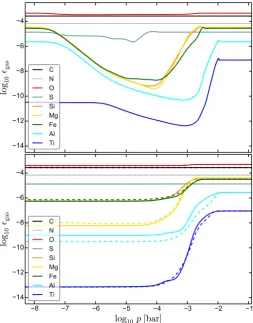
Element abundances: Figure4compares the resulting gas

ele-ment abundances. We see a strong depletion of condensable el-ements in the main cloud layer in all three models, by up to 5 orders of magnitude, concerning elements Ti, Al, Mg, Si, Mg and Fe. However, the details are different. The previous Drift model is featured by minimums ofkthat are similar in depth as compared to the overall decrease ofkin the DiffuDrift mod-els. High up in the atmosphere, where cloud particles are virtu-ally absent, there is no surface to condense on, and so the in-stantaneous mixing assumption in the D_riftmodels causes a re-increase ofktoward the top of the atmosphere, unless the ele-ment can form nuclei. In the extremely low density gas at these heights, these nuclei simply fall through the atmosphere with-out much interaction, whereas elements, which cannot nucleate, accumulate.

In contrast, in the new DiffuDriftmodels, the abundances of all elements involved in cloud formation decrease with height in a monotonic way. This behaviour is expected in the final, time-independent, relaxed state of the atmosphere as discussed in Sect.3.1. In the stationary case, the downward transport of con-densable elements via the falling cloud particles must be com-pensated by an upward diffusive transport of these elements in the surrounding gas, which implies negative element abundance gradients throughout the cloudy atmosphere, see Eq. (29). The

8 7 6 5 4 3 2 1

log

p

[bar]

12 10 8 6 4

lo

g

²

N O S Si Mg Fe Al Ti

8 7 6 5 4 3 2 1

log

p

[bar]

12 10 8 6 4

lo

g

²

N O S Si Mg Fe Al Ti

Fig. 4.The impact of our assumptions about the mixing processes in the

atmosphere on the resulting gas element abundances, in models with the same parameters as in Fig.3. Theupper plotshowsgas_k for instanta-neous mixing as assumed in the previous Driftmodel. Thelower plot

shows the results according to the new D_iffuD_riftmodels, where the full lines show the results for gas and dust diffusion, and the dashed lines show the results for gas diffusion only.

total drop of element abundances is deepest for Ti, but less deep for Si and Fe as compared to Mg.

Freytag et al. (2010) performed two-dimensional radiation

hydrodynamical simulations of substellar atmospheres which in-cluded a time-dependent description for the formation of a single kind of cloud particles for a fixed concentration of seed particles. The paper discusses substellar objects withTe_ff=900 K−2800 K,

log(g)=5 and solar element abundances. Their Fig. 9 (bottom left panel) shows the fraction of condensable gas in the atmo-sphere as a function of pressure, very similar to our Fig.4(lower plot). These results of Freytag et al. support our new DiffuDrift results, where abundances of condensable elements in the gas phase are decreasing fast in the cloud layers, and stay about constant above the clouds. We note that Freytag et al. have pre-scribed the number of seed particles and considered only one generic condensate in their simulations.

Cloud particle composition: Figure5shows the corresponding

8 7 6 5 4 3 2

log

p

[bar]

2.0 1.5 1.0 0.5 0.0

vo

lu

m

e

fr

ac

ti

on

lo

g

b

s

DRIFT

TiO2 Al2O3 CaTiO3 Fe

FeO Fe2O3 FeS MgO

Mg2SiO4 MgSiO3 SiO SiO2

8 7 6 5 4 3 2

log

p

[bar]

2.0 1.5 1.0 0.5 0.0

vo

lu

m

e

fr

ac

ti

on

lo

g

b

s

DIFFUSION (gas and particles)

8 7 6 5 4 3 2

log

p

[bar]

2.0 1.5 1.0 0.5 0.0

vo

lu

m

e

fr

ac

ti

on

lo

g

b

s

DIFFUSION (gas only)

Fig. 5.The material volume composition of the cloud particlesbs ₌

Ls

3/L3=Vs/Vtotfor the same three models as discussed in Figs.3and4.

1. A layer containing only the most stable metal-oxides at the cloud base, in this model Al2O3[s], TiO2[s] and CaTiO3[s].

The position of the cloud base, which depends onTeff and

logg, is located at around 1800 K in this model.

2. A thin layer of cloud particles around 1500 K which mainly consist of metallic Fe[s].

3. Main silicate cloud layer composed of Mg2SiO4[s],

MgSiO3[s], MgO[s], SiO[s] and SiO2[s], mixed with

metal-lic iron, upward of about 1400 K in this model.

4. Less stable solid materials such as FeS[s], FeO[s] and Fe2O3[s] are incorporated into the silicate cloud particles at

temperatures lower than about 1100 K, 1000 K and 850 K, respectively, in this model.

5. Pure nuclei at the top, here TiO2[s], which fall through the

atmosphere so quickly that they practically do not grow.

Further inspection shows, however, that the material composi-tion of the main silicate cloud layer (3) differs substantially be-tween the Driftand the DiffuDriftmodels. In the new diffusive D_iffuD_riftmodels, the first magnesium-silicate to form is fos-terite Mg2SiO4[s], which has a stoichiometric ratio Mg : Si=2 : 1.

The formation process of Mg2SiO4[s] stops once the reservoir

of Mg is exhausted, still leaving about half of the available Si in the gas phase. Since the mixing is diffusive, very little Mg

1400 1600 1800 2000 2200 2400 2600 2800

T

[K]

10 8 6 4 2

lo

g

Σ

[g

/

cm

2

]

TiO2 Al2O3 MgSiO3

Mg2SiO4 SiO SiO2

Fe FeS FeO

MgO Na2S

Fig. 6.Column densities [g/cm2_{] of different condensates in the}

atmo-sphere along a sequence of models with decreasingTeff but constant logg=3 andβ0₌

1. A value of 10−3_g/cm2_{roughly corresponds to an} optical depth of one at a wavelength ofλ=1µm (see AppendixE).

can be mixed upwards through these Mg2SiO4[s] clouds. Thus,

the remaining amount of Si above the Mg2SiO4[s] clouds

prefer-entially forms other silicate materials, in particular SiO2[s] and

SiO[s], but only very little MgSiO3[s]. This is different in our

previous Driftmodel where the depleted elements are assumed to be instantly replenished at similar rates, in which case both Mg2SiO4[s] and MgSiO3[s] are found to be about equally

abun-dant condensates in the main silicate cloud layer.

Another difference concerns FeS[s] (troilite). FeS[s] is found to form in large quantities in the previous Driftmodels, causing Sto drop significantly, see upper part of Fig.4. However, this

depends on our assumptions about how the elements are replen-ished. In the new diffusive models, upward mixing of gaseous Fe is rather inefficient because the Fe atoms have plenty of oppor-tunity to condense in form of Fe[s] on existing cloud particles along their way upwards in the atmosphere. Once the tempera-ture is low enough to allow FeS[s] to form, there is so little Fe left in the gas phase that the S abundance is more or less unaffected by FeS[s] formation, and therefore sulphur remains available for other condensates to form.

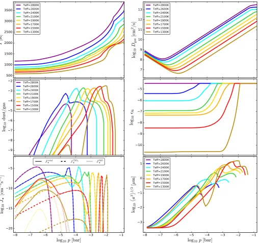
5.2. Cloud structures as function ofTeff

In this section, we study the results of a sequence of the new Dif -fuDriftcloud formation models with decreasing effective tem-perature Teff. We are using a slightly different chemical setup

here that will allow us to discuss secondary cloud layers. We consider four nucleation species (TiO2)N, (SiO)N, (KCl)N and (C)N. The nucleation rates of TiO2, KCl and C are calculated by

modified classical nucleation theory (Helling et al. 2017; Gail

et al. 1984), with a surface tension value for KCl from (Lee et al.

2018). The nucleation rate of SiO is calculated according to (Gail

et al. 2013). We have 16 elements in this setup (H, He, Li, C, N,

O, Na, Mg, Si, Fe, Al, Ti, S, Cl, K, Ca), 14 condensed species (TiO2[s], Al2O3[s], MgSiO3[s], Mg2SiO4[s] ,SiO[s], SiO2[s],

8 7 6 5 4 3 2 1

log

p

[bar]

500 1000 1500 2000 2500 3000 3500

T

[K

]

Teff=2800K Teff=2600K Teff=2400K Teff=2100K Teff=1900K Teff=1700K Teff=1500K Teff=1300K

8 7 6 5 4 3 2 1

log

p

[bar]

7 8 9 10 11 12 13

lo

g

D

s

[c

m

2

/

s]

Teff=2800K Teff=2600K Teff=2400K Teff=2100K Teff=1900K Teff=1700K Teff=1500K Teff=1300K

8 7 6 5 4 3 2 1

log

p

[bar]

9 8 7 6 5 4 3 2

lo

g

du

st

/

ga

s

Teff=2800K Teff=2600K Teff=2400K Teff=2100K Teff=1900K Teff=1700K Teff=1500K Teff=1300K

8 7 6 5 4 3 2 1

log

p

[bar]

10 9 8 7 6 5

lo

g

²

8 7 6 5 4 3 2 1

log

p

[bar]

20 15 10 5

lo

g

J

[c

m

−

3

s

−

1

]

Jtotal _JTiO2 JSiO

8 7 6 5 4 3 2 1

log

p

[bar]

3 2 1 0 1

lo

g

a

3

® 1/

3

[

µ

m

]

Teff=2800K Teff=2600K Teff=2400K Teff=2100K Teff=1900K Teff=1700K Teff=1500K Teff=1300K

Fig. 7.Sequence of cloud forming models with decreasingTeffat constant logg=3 and mixing powerlaw indexβ0=1.Top row:gas temperature

T and diffusion coefficientDgasas function of pressure (both assumed).Middle low:resulting dust to gas mass ratio and element abundance of silicon in the gas phaseSi.Lower row:resulting nucleation ratesJ?and mean particle sizesha3i1/3.

308 molecules and 50 surface growth reactions. Molecular equi-librium constants and Gibbs free energies of the condensates are all taken fromWoitke et al.(2018). Dust diffusion is included in all models.

Figure6shows the total column densities of selected cloud materialsΣs[g/cm2] in a series of DiffuDriftmodels with con-stant logg=3 and mixing indexβ0_{=1, but decreasingT}

e_ff. The

column densities of the condensed species are computed as

Σs= Z

ρsρL₃sdz, (35)

whereρs[g/cm3] is the material density of the pure condensate of kind sandρLs

3[cm

3_/cm3_{] is the volume of condensed kind}

sper volume of atmosphere. For example, forTeff=1800 K we

find of order 10 mg condensates per square centimetre, mostly

made of Mg2SiO4[s], Fe[s] and Al2O3[s], followed by SiO[s]

and MgSiO3[s].

On the left side of this plot, the first model that shows con-densation appears atTeff =2800 K. Here, the temperatures are

too high to have any other condensates than just the most sta-ble metal-oxides in form of Al2O3[s] and TiO2[s]. In the next

few models down to Teff = 2000 K, the main silicate layer

forms, mixed with iron. In this range of effective temperatures, Al2O3[s] still has the largest column density because the metal

oxide layer is situated deeper in the atmosphere where the den-sities are higher. Only forTe_ff <2000 K, the silicate-iron layer

starts to dominate by mass. At the very end of the sequence, for

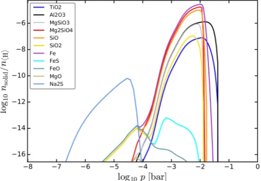
Teff<1500 K we find the first models which host a third cloud

layer made of di-sodium sulfide Na2S[s].

Figure 7 shows a few more details from this Teff-series of

at-mospheric density/temperature structures assumed (taken from the Drift-Phoenixatmosphere grid (Dehn et al. 2007; Helling

et al. 2008b;Witte et al. 2009,2011). The kinks in deep layers

(T ∼2500−3000 K) indicate the beginning of the convective layer (Schwarzschild criterion for convective instability). The upper right plot shows the assumed diffusion coefficient in the atmosphere, which decreases with Te_ff, because the convective

layer sinks into deeper layers, hence the spatial distance to the source causing the mixing motions in the atmosphere increases. The left middle plot in Fig.7shows the dust-to-gas mass ra-tio, which has its maximum in the main silicate-iron layer, and a shoulder on the right due to the deeper metal-oxide clouds which are made of the rarer elements with the highest condensation temperatures, namely aluminium, calcium and titanium. AsTeff

decreases, both layers move inward to deeper layers and become successively more narrow, until finally, forTeff=1400 K, a new

cloud layer occurs which mainly consists of di-sodium sulfide Na2S[s]. The right middle plot shows how the silicon abundance

in the gas phase is affected. All curves are monotonic decreas-ing towards the surface, with higher Si depletions for lowerTeff

where the silicate cloud particle formation is more complete. The nucleation rates of (TiO2)Nand (SiO)Nparticles are

de-picted in the lower left plot. A complicated, double-peaked pat-tern shows, which has a minimum around the main peak of the dust-to-gas ratio (at the peak position of the main silicate-iron layer). (TiO2)Nis usually the most significant nucleation species, but cooler models show additional contributions by (SiO)N. The resulting mean particle sizes are plotted on the lower right, with a tendency to produce larger particles deep in the atmosphere for lowerTeff. An in-between minimum in particle size occurs where

the main silicate material evaporates. Only the coolest model has a second minimum where Na2S[s] evaporates. Interestingly, the

hottest and the coolest model in Fig.7show about equally large cloud particles at high altitudes, whereas all other models show smaller particles.

6. Summary and Discussion

This paper has introduced a new cloud formation model appli-cable to the atmospheres of brown dwarfs and gas giant (exo-)planets. We have combined our previous cloud particle mo-ment method (Woitke & Helling 2004;Helling & Woitke 2006;

Helling et al. 2008c) with a diffusive mixing approach, according

to which, in the final relaxed time-independent state of the atmo-sphere, fresh condensable elements are diffusively transported upwards to replenish the upper atmosphere via a combination of turbulent (eddy) mixing and gas-kinetic diffusion. Our formula-tion of the problem arrives at a system of about 30 second order partial differential equations of reaction-diffusion type, where the formation and growth of the cloud particles follows from a kinetic treatment in phase-non-equilibrium.

Model setup: The new cloud formation model is applied to a

given one-dimensional (p,T) atmospheric structure in this pa-per. The model is calculated time-dependently, using an oper-ator splitting technique. All models are found to relax toward a time-independent, stationary solution, where the condensable elements are constantly mixed up diffusively, cloud particles nu-cleate from the gas phase high in the atmosphere, grow by the simultaneous condensation of different solid materials on their surface, and then decent through the atmosphere due to gravita-tional settling, before the particles stepwise purify and eventu-ally sublimate completely at the cloud base.

Fig. 8. Concentration of condensed species in a model with Teff =

1300 K, logg=3 andβ0₌₌

1, showing a secondary cloud layer almost entirely made of di-sodium sulfide Na2S[s]. nconds =ρL

s

3/V

s

mat[cm −3_{] is} the number density of solid units of condensed speciess,Vs

mat=ms/ρsis

the volume occupied by one unit of solidsin the pure material, andms

is the mass of one such units, for example 100.4 amu fors=MgSiO3.

ns

cond/nhHiis directly comparable to element abundances.

Timescales: The real-time simulation time required to reach

that stationary solution varies between a few months to several tens of years, depending on log(g) and Teff. The relaxation is

quicker when models are started from an atmosphere that is de-void of any condensable elements att=0. These relatively long simulation times make these models computationally expensive (of order 500 CPU-hours per model), because the intrinsic nu-cleation and growth reactions are very fast, which means that the models need to be advanced on short computational time steps of the order of seconds to guarantee numerical stability. The long physical timescales involved in the simulations are (i) the overall settling time for small particles inserted high in the atmosphere, and (ii) the overall mixing time for gas parcels to diffusively reach the highest point in the model from the cloud base. This implies that 3D simulations of cloud formation (GCM models, for exampleFreytag et al. 2010;Lee et al. 2016;Lines

et al. 2018a;Powell et al. 2018;Charnay et al. 2018) must be

ad-vanced for similar real-time simulation times before a relaxed physical structure can be expected. However, how long these physical timescales actually are will depend on the exact for-mulation of mixing and setting in the GCM models.

Cloud density and particle sizes: In comparison to our

previ-ous Driftmodels, the DiffuDriftmodels show fewer but larger cloud particles, which are more concentrated towards the cloud base. However, the physical properties of the cloud particles in the main silicate-iron layer towards the bottom of the clouds (dust to gas mass ratio, particle sizes, optical depth, chemical composition, etc.) are found to be similar to the results of the previous models. The dust-to-gas ratio in the main silicate-iron layer reaches a peak value of about 0.002 to 0.003, quite inde-pendent ofTeff, for not too hot models (Teff>2500 K). This is