Implementation of a multi level Power Electronic Inverter library in Modelica

Power Electronic Inverter Library in Modelica

C.I. Hill

P. Giangrande

C. Gerada

S.V. Bozhko

University of Nottingham

Aerospace Technology Centre, Innovation Park, Nottingham. NG7 2TU. UK.

[email protected]

[email protected]

Abstract

This paper presents a newly developed Power Electronic Inverter library in Modelica. The library utilises a multi-level approach with increasing model complexity at progressively higher levels. All levels are fully interchangeable so as to provide a flexible library able to be utilised for investigation at single or multiple levels of complexity. Within this inter-changeable multi-level approach, there are two key attributes which are implemented into this new library. The first is the ability to include losses between the input and output of the Power Electronic Inverter. This is implemented so that the losses are included irrespective of the direction of power flow. Secondly, this library also provides the ability to trigger single or multiple open and short circuit faults within the Inverter. The library therefore provides an extremely useful tool able to compare system response under a variety of operational scenarios.

Keywords: Inverter; Multi-Level; Losses; Faults; Actuator

1 Introduction

Power Electronic Inverters convert DC electrical power to AC. They are a vital part of the modern world and are becoming increasingly common due to the electrification of modern transport systems. They are used to drive the electrical machines within elec-tric vehicles [1] and are an essential part of electri-cally driven actuator systems within the More Elec-tric Aircraft [2]. Indeed the adoption of elecElec-trically driven actuators is becoming widespread among air-craft manufacturers due to the evident benefits in terms of efficiency, weight and maintenance [3]. However, despite the high efficiency of these electri-cal systems and low probability of fault occurrence, it is still essential to consider the losses that do occur and the effect of fault conditions. The Inverters

library presented here provides the ability to include losses, analyse thermal response and introduce fault conditions into the modelling environment. It also gives the user multiple interchangeable models of the Power Electronic Inverter in order to allow analysis at multiple levels of complexity. This is a new approach as the MSL, SPOT, Smart Electric Drives and Modelon’s ElectricPower libraries do not provide this flexible multi-level approach with loss and fault capability [4][5]. The Inverterslibrary presented here forms part of an overall Actuator

library developed as part of Actuation 2015 [6]. For an overview of the entire Actuator library please see [7]. However the purpose of this paper is to give in- depth detail on the multi-level modelling of the Power Electronic Inverter.

At first the library structure will be presented along with a definition of the multiple modelling levels. Details of the individual models will be given includ-ing both commonalities and differences. Simulation results will be shown in order to demonstrate results which can be obtained using the 5 modelling levels.

2 Multi-level definition

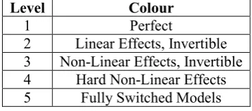
Before detailing the actual models a definition of each modelling level must be given. This is defined in line with the overall definition established by all partners within Actuation 2015 [6]. Table 1 shows the agreed definitions which are used throughout the

Actuator library [7] and are also used within this

Inverterslibrary.

Level Colour

1 Perfect

2 Linear Effects, Invertible 3 Non-Linear Effects, Invertible 4 Hard Non-Linear Effects 5 Fully Switched Models

In addition common colour coding was agreed for each modelling level as detailed in Table 2.

Level Colour

1 Red

2 Blue

3 Grey

4 Green

5 Dark Yellow

Table 2: Colour coding of each modelling level.

3 Structure

Figure 1 shows the structure of the Inverters

library.

Figure 1: Structure of theInverterspackage.

The Inverters package provides 5 levels of complexity in line with the multi-level definitions detailed in Section 2. As can be seen from Figure 1 the package is split into the NonSwitching

package and the Switching package. The Non-Switching package provides colour coded models for levels 1 to 4 and the Switching

package provides the level 5 model. Each level has a corresponding example of its use. The colour and level assignment of each model is in line with the definition of the modelling levels for the overall

Actuator library as detailed previously in Section 2. The colours for each level and the icons for Non-SwitchingandSwitchingmodels are extended from the Inverters.Utilities.Icons

package.

4 Model Interfaces

A central feature of this Inverters library is that each modelling level is fully replaceable with one another. In order for each modelling level to be fully interchangeable a common interface is used for all 5 modelling levels.

The electrical interfaces adopted for the DC interface are the Modelica Standard Library (MSL) Posi-tivePin and NegativePin. On the AC side a

PositivePlug, is used and it is assumed that a 3 phase AC side is used. A RealInput[3]is used for input of the 3 phase AC voltage demands. If closed loop control is used then the

RealInput[3] input signals should be the un-modulated outputs of the current controller. A

PartialConditionalHeatPort is used as a thermal interface for all levels. These interfaces are defined and then extended from the package Actu-ator.Electrical.Interfaces.

5 Non-Switching

5.1 Theoretical basis

There are two assumptions which are used as the basis of creating the NonSwitching package of Inverter models. The first assumption is that the AC output voltage signals, which in a Switching Inverter would be created via Pulse Width Modulation, are ideally created with a pure fundamental frequency exactly as demanded by the control signals. As such the un-modulated voltage demand signals can be used to ideally create the electrical Inverter output voltages. Within Modelica this simply means taking the 3 phase demand RealInput[3] and connect-ing it to a MSL SignalVoltage model, with m=3. This forms the initial basis of the Inverter model on the AC side and is constant throughout all the Inverter models within the NonSwitching

package. Figure 2 shows this along with the inclu-sion of the second assumption detailed below.

The second assumption which forms a basis of the

NonSwitching package is the power equivalence principle. This assumes that the power input to the Inverter is equal to the power output from the Inverter. As one side of the Inverter is AC and one is DC then:

In addition as:

PDC= IDCVDC (2)

Therefore substituting (2) into (1):

IDCVDC= PAC (3)

Where PDCis the Inverter DC side power, PAC is the Inverter AC side power, IDC is the Inverter DC side current and VDCis the Inverter DC side voltage.

Now, as both the AC power and the DC voltage can be measured, this means the DC current can be calculated by:

I

=

The AC power is measured on the AC side using a MSL PowerSensor model with m=3. The DC voltage is measured using the MSL VoltageSen-sor model. However only the absolute value of the DC voltage is required and so a MSLAbs model is used. The calculated DC current is output using a MSL SignalCurrent model. This structure therefore creates the Level 1 Inverter and is the basis for the Level 2, 3 and 4 Inverters. It is summarised in block form in Figure 2. No thermal response is in-cluded within Level 1 as no losses exist.

Figure 2: Basis of the Level 1 Inverter.

5.2 Losses

This sub-section now builds on the details given in Section 5.1 in order to create the level 2, 3 and 4 Inverter models.

To begin, it is important to note that all the Power Electronic Inverter models are fully multi-directional. As a result losses are implemented whether power flow is from the DC side to the AC

side or from the AC side to the DC side. Hence if power flow is from DC to AC the AC side power will be lower than the DC side and vice versa. This is made inherent within Levels 2, 3 and 4 by use of the MSL models shown in Figure 3. As can be seen from Figure 3Sign is used to detect the sign of the AC power. This is then used, along with Switch and

GreaterEqualThreshold, with threshold=0, in order to switch between two Constant sources. The Constant sources provide two differing val-ues dependent on the efficiency of the Inverter and the direction of power flow as will be detailed below.

Figure 3: Basis of the Level 2 Inverter.

Irrespective of the direction of power flow, in order to calculate both the Inverter losses and the DC power the same power equivalence principle is used as detailed in Section 5.1. However, as Inverter efficiency is now included, (1) is now modified.

When power flow is from the DC side to the AC side (1) becomes:

ηPDC= PAC (5)

Where η is the efficiency of the Inverter.

When power flow is from the AC side to the DC side (1) becomes:

PDC = ηPAC (6)

Efficiency is defined as:

η =୔ో౑౐ౌ౑ ౐

୔౅ొ ౌ౑౐ (7)

And:

P୓୙୘୔୙୘= P୍୒୔୙୘− P୐୓ୗୗ୉ୗ (8)

WhereP୓୙୘୔୙୘is output power,P୍୒୔୙୘is input power

andP୐୓ୗୗ୉ୗis the power lost from the device between

input and output.

Substituting (8) into (7) gives:

η =୔౅ొ ౌ౑౐ି୔ైో౏౏ు౏

୔౅ొ ౌ౑౐ (9)

Making PLOSSESthe subject gives:

P୐୓ୗୗ୉ୗ= P୍୒୔୙୘(1 − η) (10)

This therefore gives power losses in terms of the input power. However using (7) and (8) the efficien-cy and hence power losses can also be defined in terms of the output power:

η = ୔ో౑౐ౌ౑౐

୔ో౑౐ౌ౑ ౐ା୔ైో౏౏ు౏ (11)

Hence in terms of PLOSSES:

P୐୓ୗୗ୉ୗ=୔ో ౑ ౐ౌ౑ ౐_ఎ (ଵି஗) (12)

Equations (10) and (12) are crucial as they define the power losses in terms of both input and output pow-er. As a result, when power flow is from the DC to the AC side the AC side is the output and (12) gives:

P୐୓ୗୗ୉ୗ=(ଵି஗)_ఎ P୅େ (13)

Whereas when power flow is from the AC side to the DC side then the AC side is the input and (10) gives:

P୐୓ୗୗ୉ୗ=(1 − η)P୅େ (14)

Within the Inverter models developed here, these two results are incredibly useful as in both cases the power losses are defined in terms of the measureable AC power and the specified efficiency. Hence, as shown in Figure 3 and described earlier, the AC power can be measured and multiplied by the coeffi-cients shown in (13) and (14) in order to find the power lost. This is implemented using two Con-stant sources which are selected depending on the direction of power flow.

Next, the DC power must also be defined in terms of the specified efficiency and AC power. Therefore if power flow is from DC to AC then (8) becomes:

P୅େ= Pୈେ− P୐୓ୗୗ୉ୗ (15)

Substituting (13) for PLOSSES and making PDC the subject gives:

Pୈେ= P୅େ+(1−η_ߟ )P୅େ (14)

Now if power flow is from AC to DC then (8) becomes:

Pୈେ= P୅େ− P୐୓ୗୗ୉ୗ (15)

Substituting (14) for PLOSSES and making PDC the subject gives:

Pୈେ= −P୅େ+ (1 − η)P୅େ (16)

If equations (14) and (16) are compared it can be seen that the only variation is the sign of the first PAC term and the coefficient of the second PAC term. Hence, as stated previously, both equations can be implemented within Modelica using twoConstant

sources which supply the coefficient terms and

Signto select between them. PACis naturally meas-ured as positive or negative byPowerSensor.

Within Modelica (14) and (16) become:

dcPower = acPower + ((1 - data.eta)/data.eta) * acPower

And:

dcPower = acPower + (1 - data.Eta) * acPower

Finally, as the DC voltage can be measured, in both cases the DC current is then calculated from the DC power using (2) and implemented in Modleica as shown on the left hand side of Figure 2.

5.3 Efficiency

The previous sub-section showed how losses are included within the NonSwitching Inverter models. All losses were specified in terms of Inverter efficiency. However within the Level 2 model this efficiency is specified in a different manner to the Level 3 and 4 models.

conditions but the efficiency is constant. As detailed in Section 5.2 these are allowed for irrespective of the direction of power flow.

Levels 3 and 4 both use non-linear efficiency charac-teristics. The user is able to specify the power range of the Inverter and also the losses within the Inverter over the specified power range. A default character-istic is also given, as shown in Figure 4 below. However accurate characteristics are recommended to be added by the user if known. The default characteristics are per unit and are scaled within the model by the specified, or default, power range.

Figure 4: Default non-linear loss characteristics

These non-linear losses are implemented using

CombiTable1D instead of Constant. Table 3 summarises the losses included in each level of the

Inverters package. The Level 5 losses will be discussed in Section 6.

Level Losses

1 None

2 Linear Losses 3 Non-Linear Losses

4 Non-Linear Losses 5 Conduction Losses

Table 3: Losses modelled within each level of the

Inverterspackage.

An example system is now used to demonstrate the use of theInverterspackage and show the varia-tion in Inverter losses between levels. The Inverter is used within a system to control the speed of a Per-manent Magnet Machine. The Inverter is fed from a MSL ConstantVoltage and supplies a MSL

SM_PermanentMagnet. An inner current loop is used with an outer speed control loop. Please note the controllers used are not part of theInverters

package. The overall system is shown in Figure 5.

Figure 5: Example use ofInverterspackage.

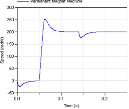
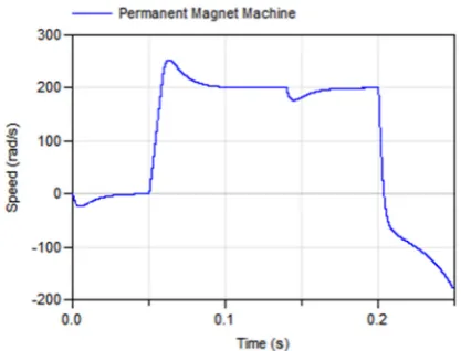
Figure 6 shows the speed response of the system when an initial load torque is demanded at 0 seconds and a step in speed from 0 to 200 rad/s is demanded at 0.05s. A further increase in load torque is demanded at 0.14s. Figure 7 shows the 3 phase AC current response.

Figure 6: Speed response

Using this response the Levels 1 to 4 Inverters

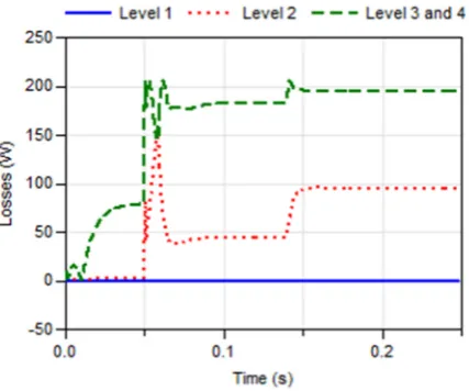
are simulated and the losses generated over the simu-lation period are compared in Figure 8.

Figure 8: Losses produced in Levels 1, 2, 3 and 4.

It can be seen from Figure 8 that the losses within the Inverter models are substantially different depending on the level of the Inverterspackage used. It can be seen how, in this case, the non-linear losses in Levels 3 and 4 are always higher. This is due to the Inverter operating at low to medium power. It can also be seen that the increase in losses at 0.14s is greater for the Level 2 Inverter than the Level 3 and 4 Inverters. At 0.14s the increase in losses in the Level 2 Inverter is greater as the losses are proportional to the Inverter power. However within the Level 3 and 4 Inverters the increase is less due to the non-linear loss characteristics meaning the Inverter efficiency is higher at higher power. This therefore shows how the inclusion of non-linear losses could be important. However, if accurate non-linear information is not known, operation is known to be in a linear region, or losses are not required then Level 1 or 2 Inverters can easily be used.

5.4 Thermal Response

The Level 2, 3 and 4 Inverter models within the

Inverters.NonSwitching package all have the same thermal implementation. As can be seen from Figure 9 a MSL PrecribedHeatFlow

model is used to convert the calculated Inverter losses into heat flow. This is connected to a

HeatCapacitor which represents the thermal capacitance of the Inverter switch modules. A

ThermalConductor is used between the

HeatCapacitor and the output PartialCon-ditionalHeatPort in order to represent the thermal resistance between the switch module and its cooling system. A

PartialCondition-alHeatPort is used so losses can still be included if no thermal output is required.

Figure 9: Thermal implementation within Levels 2, 3 and 4 Inverter models.

The user may specify the thermal parameters for the switch modules. All the required values can be read directly from module data sheets. If no user specified value is given then default values are used.

5.5 Fault

As detailed in the introduction the Inverters

library presented here forms part of an overall

Actuator library developed as part of Actuation 2015 [6]. A crucial aspect of the Actuator library is the inclusion of fault conditions within all the component models. In the case of the Power Electronic Inverters these are mainly included within the level 5 Switching model as no switches exist within the lower level models. However within the Level 4 Inverter a full bridge fault is possible. When triggered the Power Electronic Inverter output becomes zero. This represents a full-bridge open circuit fault or deactivation of the Inverter.

Figure 10 shows the speed response of the same system as shown in Figure 5. However in this case the Level 4 Inverter model is used and a full-bridge fault is triggered at 0.2s. Figure 11 shows the AC voltage response and Figure 12 shows the Inverter output power.

Figure 11: Faulted 3 phase voltage response

Figure 12: Faulted Inverter power response

It can be seen from Figures 10 to 12 that when the fault is triggered at 0.2s the Inverter output becomes 0. Therefore the output voltage and power both become 0 as shown in Figures 11 and 12. Within Figure 10 the speed response shows how, after the fault is triggered, the Permanent Magnet Machine accelerates in the negative direction due to the load torque acting as a mechanical source.

Table 4 summarises the fault conditions included in each level of theInverterspackage. The Level 5 faults will be discussed and shown in Section 6.

Level Faults

1 None

2 None

3 None

4 Full-Bridge

5 Single Switch, Single Phase, Multi-Phase and Full Bridge

Table 4: Fault conditions modelled within each level of theInverterspackage.

The Failure Triggering Toolbox detailed in [7][8] is used within the models in order to trigger the required faults. A Boolean coding system is used to trigger the faults where 0 = normal operation, 1 = faulted operation. The faults can be implemented at any time instant but must be defined pre simulation.

6 Switching

6.1 Model Basis and Sub-Components

The Level 5 Inverter model within the Invert-ers.Switchingpackage is based on the 6 switch, 3 leg topology shown in Figure 13. The switches are numbered S1 to S6 according to the order of switch-ing. Each has a corresponding parallel diode.

Figure 13: Topology used the for Invert-ers.Switchingpackage

In order to build the Level 5 Inverter certain sub-components were needed. These are contained in

Inverters.Switching.SubComponents

and include FaultSwitch, PulseWidthModu-lation andFaultInjector.

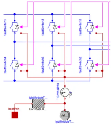
FaultSwitch is a model which represents the parallel switch and diode combination shown in Figure 13. Figure 14 shows how FaultSwitch is used within the Level 5 Inverter in order to create the topology shown in Figure 13.

Figure 15 shows the MSL models used within

FaultSwitch. An IdealClosingSwitch

MSL model is used as the main switch for power conversion. It receives a Boolean signal which dictates whether the switch is open or closed. In series with this switch is a VariableResistor. Under normal conditions the resistance of this

VariableResistor is set to be a magnitude of 10-6 _{smaller than the IdealClosingSwitch} resistance when conducting. It therefore has negligi-ble effect. However this VariableResistor is mainly included for use under fault conditions. As the IdealClosingSwitch resistance is very small, under short circuit conditions a very large current is obtained. In order to counteract this, the user is able to limit the short circuit current by defin-ing a larger short circuit resistance. The Varia-bleResistor is therefore used to introduce this larger resistance under fault conditions. A Boole-anToReal MSL model is used as an input to the

VariableResistor. This controls the resistance value as it receives a Boolean control signal which is false under normal operation and true under faulted operation. This does mean that the resistance also increases during an open circuit fault; however this has negligible effect due to the open circuit. The Boolean control signal comes from another

Inverters.Switching sub-component named

FaultInjector which will be detailed later in this section.

In parallel with the IdealClosingSwitch is an

IdealDiode. The diode is uncontrolled and has default parameters, although these can also be speci-fied by the user. This diode is also in series with the

VariableResistor detailed above. As a result the increased resistance during short circuits, as detailed above, also affects the current path through the diode. During open circuit faults the combination of the diode and increased resistance provides a path for the release of otherwise trapped energy. If both paths were instantaneously open circuited then an extremely large voltage spike would be produced due to trapped energy. In a practical system this would result in sparks as the air would conduct under high voltage. However, in order to avoid these numerical spikes in this model the diode is allowed to briefly conduct.

Figure 15: Inverters. Switching. Sub-Components.FaultSwitch

The PulseWidthModulation sub-component implements sine-triangle Pulse Width Modulation in order to create the 6 required switching signals. The user is able to specify the switching frequency and also the modulation index. In order to make all 5 modelling levels interchangeable the voltage demand signals which are input to the Level 5 Inverter are required to be un-modulated as was the case for Levels 1 to 4.

Finally, the FaultInjector sub-component is simply used to override the Pulse Width Modulated switching signals when a fault is triggered by the user. Under normal operation the switching signals are fed through the FaultInjector unchanged however when a fault is triggered the Pulse Width Modulated switching signals are blocked and the relevant fault state is output to the relevant switches. In addition the FaultInjector sub-component also generates the Boolean control signal which dic-tates the resistance of the VariableResistor

contained within FaultSwitch. Boolean logic is used to create the relevant signal required to increase the resistance of the VariableResistor during faulted operation.

The Failure Triggering Toolbox detailed in [7][8] is used within FaultInjector in order to trigger the required faults. An Integer coding system is used to trigger the faults where 0 = normal operation, 1 = short circuit and 2 = open circuit. The faults can be implemented at any time instant but must be defined pre simulation.

6.2 Faults

Figure 16: Speed response with a single phase open circuit fault at 0.2s

Figure 17: Current response with a single phase open circuit fault at 0.2s

Figures 16 and 17 show the effect of introducing a single phase fault. It can be seen that after the fault occurs the speed demand is still roughly maintained but with a lot of ripple and the faulted phase current falls to 0. The small current on the faulted phase is due to the dissipation of trapped energy as explained in Section 6.1.

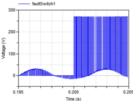
Figure 18: Voltage over FaultSwitch1 with a short circuit fault at 0.2s

Figure 19: Current through FaultSwitch1 with a short circuit fault at 0.2s

Figures 18 and 19 show the effect of a single switch short circuit fault. Figure 18 shows the voltage over the switch. As expected, before the fault the voltage follows the Pulse Width Modulation signals but after the fault it is shorted to 0. Figure 19 shows the current through the same switch. As detailed in Section 6.1, this is limited by the specified short circuit resistance. In this case the specified short cir-cuit resistance is 1Ω and as VDC is 270V then the short circuit current is 270A. It can be seen that during the cycles of the Pulse Width Modulation where the switch should be open it continues to operate correctly.

Figure 20 shows the current response for a full bridge open circuit. As expected all 3 phase currents fall to 0 when the fault is triggered at 0.2s. Finally, Figure 21 shows the speed response for a full bridge short circuit. As with the faulted speed response for the Level 4 Inverter, shown in Figure 10, the Perma-nent Magnet Machine accelerates in the negative direction after the fault is triggered due to the load torque acting as a mechanical source.

Figure 21: Speed response with short circuit at 0.2s Overall this section has shown how there are a wide range of fault conditions which can be easily intro-duced and investigated using the Level 5 Inverter. This again emphasises the flexibility of the

Inverterslibrary presented here.

6.3 Losses

The Level 5 Switching model includes the conduction losses of the switch and when conduct-ing. Energy losses due to switching are neglected. As can be seen from Figure 15 theFaultSwitch sub-component contains a HeatPortwhich outputs the heat flow generated from the switch and diode con-duction losses to the Switching model. These outputs are then all connected to the inputs of a

ThermalConductorandHeatCapacitor.

6.4 Thermal response

The Level 5 Switching model uses the MSL

ThermalConductor, HeatCapacitor and

PartialConditionalHeatPort as detailed for Levels 1 to 4 within Section 5.4. No Pre-cribedHeatFlow model is needed as the switch and diode conduction losses are already in the form of heat flow. However a HeatFlowSensor is included to give the user a numerical representation of the losses within the Level 5 Inverter.

7 Conclusion

This paper has presented a newly developed Power Electronic Inverter library in Modelica. This library utilises a multi-level approach which gives a high level of flexibility according to the user’s needs. All levels are fully interchangeable and provide multi-directional power flow. In addition this new library gives the user the ability to include multi-directional

losses at different levels of accuracy while also providing the ability to introduce a multitude of Power Electronic Inverter fault conditions.

Overall this library is an extremely flexible multi-level tool which provides Power Electronic Inverter models that can be easily inserted, parameterised, interchanged and adapted to the user’s requirements.

8 Future

At present the whole Actuation 2015 Actuator

library, which includes this Inverters library, is in the process of experimental verification. The future availability and licensing of this library is also currently under discussion within the consortium.

References

[1] Assadian, F.; Fekri, S.; Hancock, M., "Hybrid electric vehicles challenges: Strate-gies for advanced engine speed con-trol,"International Electric Vehicle Confer-ence (IEVC), 2012.

[2] Naayagi, R.T., "A review of more electric aircraft technology,"Energy Efficient Tech-nologies for Sustainability (ICEETS),2013. [3] A. Boglietti et al. “The safety critical electric

machines and drives in the more electric air-craft: A survey”, in IEEE Industrial Elec-tronics Conference, 2009.

[4] J. V. Gragger, et al. “The SmartElec-tricDrives Library – powerful models for fast simulations of electric drives,” Proceedings of the 5th International Modelica Confer-ence,pp. 571–577, 2006.

[5] R. Rai, et al. "Simulation-Based Design of Aircraft Electrical Power Systems." Proceed-ings of the 8th Modelica Conference. 2011. [6] Funded by the European Commission within

the Seventh Framework Program under grant FP7-284916http://www.actuation2015.eu/ [7] Van der Linden, F., Schlegel, C.,

Christ-mann, M., Regula, G., Hill, C.I., Giangrande, P., Mare, J.C., Egaña, I. “Implementation of a Modelica Library for Simulation of Elec-tromechanical Actuators for Aircraft and Helicopters.” Proceedings of the 10th Inter-national Modelica Conference. 2014.