A Rank One Fitting Method with Descent Direction for Solving Symmetric Nonlinear Equations

(1)

A Rank-One Fitting Method with Descent Direction for

Solving Symmetric Nonlinear Equations

*

Gonglin YUAN, Zhongxing WANG, Zengxin WEI

College of Mathematics and Information Science, Guangxi University, Nanning, Guangxi, China Email: [email protected].

Received January 14, 2009; revised March 4, 2009; accepted May 31, 2009

ABSTRACT

In this paper, a rank-one updated method for solving symmetric nonlinear equations is proposed. This method possesses some features: 1) The updated matrix is positive definite whatever line search technique is used; 2) The search direction is descent for the norm function; 3) The global convergence of the given method is established under reasonable conditions. Numerical results show that the presented method is in-teresting.

Keywords: Rank-One Update, Global Convergence, Nonlinear Equations, Descent Direction

1. Introduction

Consider the following system of nonlinear equations: ( ) 0, n,

F x  x R (1) where F:Rn_→_Rn_{is continuously differentiable and the}

Jacobian ▽F(x) of F(x) is symmetric for all x∈Rn_{. Let} θ(x) be the norm function defined by

2 1

( ) ( )

2

x F x

 

then the nonlinear Equation (1) is equivalent to the fol-lowing global optimization problem

min ( ),_ _{x x R}_ n (2) The following iterative method is used for solving (1)

k k k

k

x

d

x

_₁







(3) where xk is the current iterative point, dk is a search

di-rection, and ak is a positive step-size.

It is well known that there are many methods [1–9] for the unconstrained optimization problems

min_{x R}_ n f x UP( )( ) ,

where the BFGS method is one of the most effective quasi-Newton methods [10–17]. These years, lots of modified BFGS methods (see [18–23]) have been pro-posed for UP. Different from their techniques, Xu [24] presented a rank-one fitting algorithm for UP and the

numerical examples are very interesting. Motivated by their idea, we give a new rank-one fitting algorithm for (1) which possesses the global convergence, the method can ensure that the updated matrices are positive definite without carrying out any line search, the search direction is descent for the normal function, and the numerical results is more competitive than those of the BFGS method for the test problem.

For nonlinear equations, the global convergence is due to Griewank [25] for Broyden’s rank one method. Fan [1], Yuan [26], Yuan, Lu andWei [27], and Zhang [28] presented the trust region algorithms for nonlinear equa-tions. Zhu [29] gave a family of nonmonotone back-tracking inexact quasi-Newton algorithms for solving smooth nonlinear equations. In particular, a Gauss- Newton-based BFGS method is proposed by Li and Fu-kushima [30] for solving symmetric nonlinear equations, and the modified methods [31,32] are studied.

The line search rules play an important role for solving the optimization problems. In the following, we briefly review some line search technique to obtain the stepsize

ak.

Brown and Saad [33] proposed the following line search method:

( ) ( ) ( )T

k k k k k k k

x d x x

     d

k

(4) where

( )T ( )T ( )

k k k

x d F x F x d



  

(0,1), ik, (0,1)

k r r

   

, ,

*_{National Natural Science Foundation of China (10761001) and the}

Scientific Research Foundation of Guangxi University (Grant No.

(2)

k

( )

( ) ( ) ( )T

k k k l k k k

x d x x

     d ,

m

( ) 0 ( )

( ) max { ( )}, (0) 0

( ) min{ ( 1), }, 1

l k j m k k j

x x

m k m k M k

  _{ }  _ 

  

and M is a nonnegative integer. Yuan and Lu [32] pre-sented a new backtracking inexact technique to obtain the stepsize ak:

2 2

( ) ( ) ( )T

k k k k k k k

F x  d  F x  F x d (5) where δ∈(0,1) is a constant, and dk is a solution of the

system of linear Equation (9). Li and Fukashima [11] give a line search technique to determine a positive step-size ak satisfying

2 2

1 2

( ) ( )

k k k k

k k k k k k

F x d F x



    

 

   2 (6)

where δ1 andδ2 are positive constants, and {ε_k} is a

positive sequence such that

0 k

k







 



(7) The Formula (7) means that {F(xk)} is approximately

norm descent when k is sufficiently large. Gu, Li, Qi, and Zhou [14] presented a descent line search technique as follows

2 2

2

1 2

( ) (

( )

k k k k

F x d F x

2 )

F x d



   

 

  (8)

whereδ1 andδ2 are positive constants. In this paper, we

also use the Formula (8) as line search to find the step-size ak:

The search direction dk: play a main role in line search

methods for solving optimization problems too, and dk: is

a solution of the system of linear equation ( ) 0

k k k

B d F x  (9) where Bk is often generated by BFGS update formula

1

T T

k k k k k k

k k T T

k k k k k

y y B s s B

B B

y s s B s

    (10)

where 1

k k

y g gk and sk xk1xk Is there another way to determine the update formula? Accordingly the search direction dk is determined by the way. In this

pa-per, the updated matrix Bk is generated by the following

rank-one updated formula

1

T T

k k k

B_ B v v_k (11)

1

1 T k k k k

k k T

k k k

H v v H

H H

v B v

   _ (12)

0

nite matrix, 1

k

B _H

k and vk  0 kF x( ),k 0

is a positive constant. Then we use the following formula to get the search direction,

1

( )

k k

B d q   0 (13)

1 1

1

( )

( ) k k k k

k

( )

F x F F x

q 





 

 (14)

Bk follows (11), ak-1 is the steplength used at the

pre-vious iteration, and the Equation (14) is inspired by [34]. Throughout the paper, we use these notations:

.

is the Euclidean norm, and F(xk) and F(xk+1) are replaced by Fk

and Fk-1, respectively.

This paper is organized as follows. In the next section, the algorithm is stated. The global convergence conver-gence is established in Section 3. The numerical results are reported in Section 4.

2. Algorithm

In this section, we state our new algorithm based on Formulas (3), (8), (11), (12) and (13) for solving (1).

Rank-One Updated Algorithm (ROUA). Step 0: Choose an initial point x0∈Rn constants

, 0 ,

1 , , 0 ), 1 , 0

(  ₀ ₁ ₂  ₁ 







_

r

symmetric positive definite matrices B0 and B0-1=H0 . Let:

k = 0;

Step 1: If F x( )_k 0, stop. Otherwise, solving lin-ear Equation (13) to get dk;

Step 2: Find ak is the largest number of {1,r,r2,…}

such that (8);

Step 3: Let the next iterative point be xk+1= xk+akdk;

Step 4: Update Bk+1 and Hk+1 by the Formulas (11) and (12) respectively;

Step 5: Set k: = k + 1. Go to Step 1.

In this paper, we also give the normal BFGS method for solving (1), the algorithm which has the same condi-tions to ROUA is stated as follows.

BFGS Algorithm(BFGSA).

In ROUA, the Step 4 is replaced by: Update Bk+1 by the Formula (10).

Remark 1. a) By the Step 0 of ROUA, there should exist constants λ1≥λ0＞0 such that

2 2

1 0

2 2

0 1

,

1 1 _,

T k

T n

k

d d B d d

d d H d d d R

 

 

(3)

b) By the Step 4 of ROUA, it is easy to deduce that the updated matrices are symmetric

3. Convergence Analysis

This section will establish the global convergence for ROUA. Let Ω be the level set defined by

0 { |x F x( ) F x( ) }

   (16) In order to establish the global convergence of ROUA, the following assumptions are needed [30,34,35].

Assumption A 1) F is continuously differentiable on an open convex set Ω1 containing Ω. 2) The Jacobian of F is symmetric, bounded and uniformly nonsingular on

Ω1, i.e., there exist constants M≥m＞0 such that

1

( ) ,

F x M x

    (17) and

1

( ) , , n

F x d m d x d R

      (18) Remark Assumption A 2) implies that

1

( ) , , n

M d  F x d m d x   d R (19)

1

9 ) ( ) , ,

M x y  F x F y m x y x y   (20)

In particular, for all x∈Ω1, we have

* _{( )} _{( )} _{( )}* *

M x x  F x  F x F x m x x (21)

where x*_{stand for the unique solution of (1) in}_Ω 1.

Lemma 3.1 Let Assumption A hold. Consider ROUA. Then for any d∈Rn_,_{then there exist constants}_m

0 such

that

2 0 ,

T n

k

d B dm d  d R (22) i.e., the matrix Bk is positive for all k.

Proof. By ROUA, we know that the initial matrix B0 is symmetric positive, and then we have (15). Using (11), for k≥1, we have

1 2 1

2

1 0

T T T T

k k k k

T T

k k

T T

k

d B d d B d d v v d

d B d d v

d B d d B d  d



 

 _  ₀

(23)

Let m0=λ0. Then we get (22). The proof is complete.

Since Bk is positive definite, then dk which is

deter-mined by (13) has the unique solution. The following lemma can found in [34], here we also give the process of this proof.

Lemma 3.2 Let Assumption A hold. If xk is not a

sta-tionary point of (2), then there exists a constant a'＞0 depending on k such that when ak-₁∈(0, a'), the unique

solution d(ak-₁) of (13) such that

1 ( )T ( ) 0

k k

x d

  _

  (24) Moreover, inequality

2 2

1 1

2

1 1 1 2 1

( ( )) ( )

( ) ( )

k k k k

F x d F x

d F              

   2

x ) k x k k (25)

Proof. By (14), we can deduce that

1 1 0 ( ) ( ) (

lim

k k k

q F x F



  

  (26)

From (13), we get

1 1 1 0 1 1 0 1 ( ) ( ) ( ). ( ) ( ) ( ). ( ) ( ) ( )

lim

k k T k k T

k k k k

T

k k k k

x d

F x F x B q

F x F x B F x F x

                       (27)

Since xk is not a stationary point of (2), we have ▽ F(xk)F(xk)≠0. By ▽F(xk) is symmetric and Bk is

posi-tive. We obtain (24).

1 1 2 2 1 1 0 1 1 0 1 ( ( )) ( )

2 ( ) ( )

2 ( ). ( ) ( ) ( ) 0

lim

k

k k k k

k T

k k

T

k k k k k

F x d F x

x d

F x F x B F x F x

                          

However, the right hand side of (25) is O(ak-₁). Thus,

inequality (25) holds for all ak-1＞0 sufficiently small.

The proof is complete.

The above lemma shows that line search technique (8) is reasonable, and the given algorithm is well defined. Lemma 3.2 also shows that the sequence {θ(xk)} is

strictly decreasing. By Lemma 3.2, it is not difficult to get the following lemma.

Lemma 3.3 Let {xk} be generated by ROUA.

Con-sider the line search (8). Then {xk} ∈Ω moreover, { ( ) }F x_k converges.

Lemma 3.4 Let Assumption A hold and

, 1 { ,_k d x_k _k_, }F_k

be generated by ROUA. Then we have 2

0 k k

k F     

(4)

0 k k k d    



(29)

Proof. By the line search (8), we get

2 2

1 1 1 2 1

2 2

1

( ) ( )

k k k k

k k d F F F   _  _   _     x (30)

Summing these inequalities (30) for k from 0 to ∞ we obtain (28) and (29). Then we complete the proof of this Lemma.

Lemma 3.5 Let Assumption A hold. Consider ROUA. Then {Bk } converges, for all k and any d∈Rn then there exist constants m0 and M0 such that

2 0 ,

T n

k

d B dM d  d R (31) and

2 2

0 0

1 T 1 _, n

k

d d H d d d R

M  m   (32)

which mean that the updated matrices are all positive by ROUA.

Proof. By the updated Formula (11), we have

2 1 2 2 0 2 2 0 0 0 T

k k k k k

k k k

k

i i i

B B v v B v

B F B F              



k (33)

By (28), we know that 2 0 k i i i F  



is convergent. Then we can deduce that {B_k } is con-vergent. So there exists a constant M0 such that

0

k

B M for all k (34) Accordingly, we get (28). By (32), (31), and the Re-mark 1(b), we can deduce that the updated matrices are all symmetric and positive. Consider 1

k k

H _B _we

ob-tain (32) immediately. So, we complete the lemma. By (32), (31), and (34), we have

1 0

0 1

( ) , ( )

k k k k k k k k

q B d M d d q

m

 _     _₁ (35)

Now we establish the global convergence theorem of ROUA.

Theorem 3.1 Let Assumption A hold and

, 1

{ ,k d xk k, }Fk be generated by ROUA. Then the se-quence {xk} converges to the unique solution x* of (1) in

0

lim

k

k F



 (36)

Proof. By Lemma 3.3, we know that {F_k } con-verges. By Lemma 3.4, we get

0

lim

k k

k

F





 (37)

then, we have

0

lim

k

k F



 (38)

or 0

lim

k k  

 (39)

Therefore, we only discuss the case of (38). In this case, for all k sufficiently large and

' k

k _r

   by (8), we obtain

2 2

2

1 2

( ' ( )

( )

k k k k

F x d F x

F x d



   

 

   (40)

By Lemma 3.3, we know that {xk}∈Ω is bounded,

considering (35), it is easy to deduce that {qk(ak-1) and

{dk} are bounded. Let {xk} and {dk(a)} converge to x*

and dx*_{, respectively. Then we have}

* 1

( ) (

lim

k k

k

q  _ 



  x) (41)

Let both sides of (40) be divided by ak' and take limits

as k→∞ we obtain

* * ( )_x T_d 0



  (42) By (31) and (13), we have

1 2 0 1 0 ( ( ) T T

k k k k k k

T

k k k

d B d q d

m d q d

        ) k (43)

As k→∞ taking limits in both of (43) yields 2

* * 0 ( )T

k

x d m d



  

This together with (42) implies d*_=0._{From (35), we}

have

1

( )

lim

k k

k

q  



0



which together with (41), we obtain * ( ) 0x



  (44) By ___{( )}_x* _{ }_{F x F x}_{( ) ( )}* * _{and using}__{F x}_{( )}* _is nonsingular, we have . This implies (36). The proof is complete.

* ( )

(5)

[image:5.595.55.539.122.396.2]

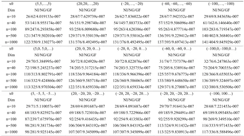
Table 1. Test results for ROUA.

x0 (5,5,…,5) (20,20,…,20) (–20,…, –20) (–60, –60,…, –60) (–100,…, –100)

Dim NI/NG/GF NI/NG/GF NI/NG/GF NI/NG/GF NI/NG/GF

n=10 40/121/8.132565e-007 43/130/8.142272e-007 43/130/8.143256e-007 45/136/9.711997e-007 47/142/6.423242e-007

n=40 43/130/7.823362e-007 46/139/8.163385e-007 46/139/8.163465e-007 49/148/6.389598e-007 50/151/6.806303e-007

n=100 44/133/8.517388e-007 47/142/8.916340e-007 47/142/8.916354e-007 50/151/7.002112e-007 51/154/7.468255e-007

n=500 46/139/8.076481e-007 49/148/8.467259e-007 49/148/8.467260e-007 52/157/6.664491e-007 53/160/7.124612e-007

n=1000 47/142/7.340784e-007 50/151/7.698173e-007 50/151/7.698173e-007 52/157/9.480059e-007 54/163/6.502176e-007

x0 (5,0, 5,0,…) (20, 0, 20, 0…) (–20, 0, –20, 0…) (–60, 0, –60, 0…) (–100,0,–100,0…)

n=10 39/118/6.440181e-007 42/127/6.456963e-007 42/127/6.458627e-007 44/133/7.690322e-007 45/136/8.088567e-007

n=40 41/124/9.581725e-007 44/133/9.998342e-007 44/133/9.998539e-007 47/142/7.823915e-007 48/145/8.333429e-007

n=100 43/130/6.657874e-007 46/139/6.969606e-007 46/139/6.969629e-007 48/145/8.555192e-007 49/148/9.121694e-007

n=500 44/133/9.861003e-007 48/145/6.615057e-007 48/145/6.615058e-007 50/151/8.129150e-007 51/154/8.675076e-007

n=1000 45/136/8.961735e-007 48/145/9.396191e-007 48/145/9.396192e-007 51/154/7.392479e-007 52/157/7.893927e-007

x0 (5, –5, 5, –5…) (20, –20, 20, –20…) (–20, 20, –20, 20…) (–20, 20, –20, 20…) (–100, 100…)

n=10 30/91/8.710675e-007 33/100/7.545800e-007 33/100/7.545800e-007 35/106/8.150523e-007 36/109/8.146625e-007

n=40 31/94/8.893379e-007 34/103/8.687998e-007 34/103/8.687998e-007 37/112/6.403068e-007 38/115/6.691432e-007

n=100 31/94/8.918405e-007 34/103/8.713106e-007 34/103/8.713106e-007 37/112/6.423164e-007 38/115/6.713147e-007

n=500 31/94/8.923155e-007 34/103/8.717867e-007 34/103/8.717867e-007 37/112/6.426974e-007 38/115/6.717265e-007

n=1000 31/94/8.923306e-007 34/103/8.718018e-007 34/103/8.718018e-007 37/112/6.427095e-007 38/115/6.717395e-007

Table 2. Test results for BFGSA.

x0 (5,5,…,5) (20,20,…,20) (–20,…, –20) (–60, –60,…, –60) (–100,…, –100)

n=10 26/62/4.019133e-007 28/67/7.629739e-007 26/62/7.836022e-007 28/67/7.942352e-007 29/69/8.843658e-007

n=40 53/141/8.955174e-007 56/151/9.298740e-007 54/145/7.883733e-007 57/152/9.506096e-007 61/162/6.146640e-007

n=100 89/247/6.293858e-007 93/258/6.009680e-007 95/263/4.620386e-007 95/263/4.877714e-007 103/283/6.719347e-007

n=500 121/347/9.502010e-007 129/371/9.550139e-007 129/371/9.550162e-007 136/391/9.229412e-007 140/402/8.368401e-007

n=1000 122/350/9.130277e-007 131/376/8.492495e-007 131/376/8.492495e-007 137/393/9.697413e-007 141/404/9.845929e-007

x0 (5,0, 5,0,…) (20, 0, 20, 0…) (–20, 0, –20, 0…) (–60, 0, –60, 0…) (–100,0,–100,0…)

n=10 29/70/5.384995e-007 30/72/8.024920e-007 30/72/8.022076e-007 31/74/7.737379e-007 32/76/6.247863e-007

n=40 72/198/5.245237e-007 74/203/5.317215e-007 74/203/5.325755e-007 75/205/6.538916e-007 75/204/9.700355e-007

n=100 110/313/8.802791e-007 118/336/9.964184e-007 118/336/9.966396e-007 125/357/9.676773e-007 128/366/8.655033e-007

n=500 116/332/9.424860e-007 126/360/9.585718e-007 126/360/9.586065e-007 133/380/9.648650e-007 136/389/9.324697e-007

n=1000 113/325/8.970304e-007 122/351/8.659330e-007 122/351/8.659334e-007 129/371/8.270087e-007 132/380/8.530508e-007

x0 (5, –5, 5, –5…) (20, –20, 20, –20…) (–20, 20, –20, 20…) (–20, 20, –20, 20…) (–100, 100…)

n=10 29/71/5.110057e-007 28/69/4.091687e-007 28/69/4.091687e-007 29/70/7.916413e-007 28/68/7.221453e-007

n=40 68/183/9.825927e-007 69/188/5.723010e-007 69/188/5.722966e-007 69/185/9.294491e-007 69/189/8.093485e-007

n=100 87/239/7.675976e-007 92/254/9.416435e-007 92/254/9.413503e-007 92/255/9.920299e-007 98/269/9.349510e-007

n=500 98/281/9.381734e-007 106/304/9.843192e-007 106/304/9.843192e-007 113/324/9.911432e-007 116/333/9.971433e-007

[image:5.595.55.540.427.698.2]

(6)

4. Numerical Results

In this section, we report results of some preliminary numerical experiments with ROUA. Problem. The dis-cretized two-point boundary value problem is similar to the problem in [36]

2 1

( ) ( )

( 1)

F x Ax T x

n

  

where A is the n×n tridiagonal matrix given by

8 1

1 8 1

1 1 8

A



 

_ _ 

 

   

  

 

 _ 

 



 

 

    

and

)) ( , ), ( ), ( ( )

(x T1 x T2 x T x T   n

with Ti(x)sinxi 1,i1,2,,n.In the experiments, the parameters in ROUA were chosen as r0.1，

. The program was coded in MATLAB Subsection 6.5.1. We stopped the iteration when the con-dition

4 0 1 2 10

 _{ }  _ 

6 0

( ) 1

F x  was satisfied.

The columns of the tables have the following mean-ing:

Dim: the dimension of the problem. NI: the total number of iterations.

NG: the number of the function evaluations. GF: the function norm evaluations.

In the next table, the numerical results are to test ROUA.

In the

Table 2,

the numerical results are to test

BFGSA

.

From these two tables, we can see that the numerical results of the two methods are all interesting. The nu-merical results of the proposed method perform better, and more stationary than the method BFGSA. Moreover, for the method ROUA, the initial points and the dimen-sion do not influence the number of iterations very much. However, for the BFGSA, the number of the iteration will increase quickly with the dimension becoming larger. One thing we like to point out is that δ0 should be chosen

in such a way that it is not too large. Overall, from the numerical results, we can see that the ROUA is one of the robust methods for symmetric nonlinear equations.

5. Acknowledgements

We are very grateful to anonymous referees and the edi-tors for their valuable suggestions and comments, which

6. References

[1] R. Fletcher, Practical meethods of optimization, 2nd Edi-tion, John Wiley & Sons, Chichester, 1987.

[2] A. Griewank and L. Toint, “Local convergence analysis for partitioned quasi-Newton updates,” Numerical Mathe- matics, No. 39, pp. 429–448, 1982.

[3] G. L. Yuan and X. W. Lu, “A new line search method with trust region for unconstrained optimization,” Com-munications on Applied Nonlinear Analysis, Vol. 15, No. 1, pp. 35–49, 2008.

[4] G. L. Yuan and X. W. Lu, “A modified PRP conjugate gradient method,” Annals of Operations Research, No. 166, pp. 73–90, 2009.

[5] G. L. Yuan, X. W. Lu, and Z. X. Wei, “New two-point step size gradient methods for solving unconstrained op-timization problems,” Natural Science Journal of Xiang-tan University, Vol. 1, No. 29, pp. 13–15, 2007.

[6] G. L. Yuan, X. W. Lu, and Z. X. Wei, “A conjugate gra-dient method with descent direction for unconstrained optimization,” Journal of Computational and Applied Mathematics, No. 233, pp. 519–530, 2009.

[7] G. L. Yuan and Z. X. Wei, “New line search methods for unconstrained optimization,” Journal of the Korean Sta-tistical Society, No. 38, pp. 29–39, 2009.

[8] G. L. Yuan and Z. X. Wei, “A rank-one fitting method for unconstrained optimization problems,” Mathematica Applicata, Vol. 1, No. 22, pp. 118–122, 2009.

[9] G. L. Yuan and Z. X. Wei, “A nonmonotone line search method for regression analysis,” Journal of Service Sci-ence and Management, Vol. 1, No. 2, pp. 36–42, 2009. [10] R. Byrd and J. Nocedal, “A tool for the analysis of

quasi-Newton methods with application to unconstrained minimization,” SIAM Journal on Numerical Analysis, No. 26, pp. 727–739, 1989.

[11] R. Byrd, J. Nocedal, and Y. Yuan, “Global convergence of a class of quasi-Newton methods on convex prob-lems,” SIAM Journal on Numerical Analysis, No. 24, pp. 1171–1189, 1987.

[12] Y. Dai, “Convergence properties of the BFGS algo-rithm,” SIAM Journal on Optimization, No. 13, pp. 693– 701, 2003.

[13] J. E. Dennis and J. J. More, “A characterization of super-linear convergence and its application to quasi-Newtion methods,” Mathematics of Computation, No. 28, pp. 549–560, 1974.

[14] J. E. Dennis and R. B. Schnabel, “Numerical methods for unconstrained optimization and nonlinear equations,” Pretice-Hall, Inc., Englewood Cliffs, NJ, 1983.

[15] M. J. D. Powell, “A new algorithm for unconstrained optimation,” in Nonlinear Programming, J. B. Rosen, O. L. Mangasarian and K. Ritter, eds. Academic Press, New York, 1970.

(7)

Optimiza-tion, Science Press of China, 1999. [27] G. L. Yuan, X. W. Lu, and Z. X. Wei, “BFGS trust-re-gion method for symmetric nonlinear equations,” Journal of Computational and Applied Mathematics, No. 230, pp. 44–58, 2009.

[17] G. L. Yuan and Z. X. Wei, “The superlinear convergence analysis of a nonmonotone BFGS algorithm on convex,” Objective Functions, Acta Mathematica Sinica, English

Series, Vol. 24, No. 1, pp. 35–42, 2008. [28] J. Zhang and Y. Wang, “A new trust region method for nonlinear equations,” Mathematical Methods of Opera-tions Research, No. 58, pp. 283–298, 2003.

[18] D. Li and M. Fukushima, “A modified BFGS method and its global convergence in nonconvex minimization,” Jour-nal of ComputatioJour-nal and Applied Mathematics, No. 129,

pp. 15–35, 2001. [29] D. Zhu, “Nonmonotone backtracking inexact quasi-New-ton algorithms for solving smooth nonlinear equations,” Applied Mathematics and Computation, No. 161, pp. 875– 895, 2005.

[19] D. Li and M. Fukushima, “On the global convergence of the BFGS methods for on convex unconstrained optimi-zation problems,” SIAM Journal on Optimioptimi-zation, No. 11, pp. 1054–1064, 2001.

[30] D. Li and M. Fukushima, “A global and superlinear con-vergent Gauss-Newton-based BFGS method for symmet-ric nonlinear equations,” SIAM Journal on Numesymmet-rical Analysis, No. 37, pp. 152–172, 1999.

[20] Z. Wei, G. Li, and L. Qi, “New quasi-Newton methods for unconstrained optimization problems,” Applied Ma- thematics and Computation, No. 175, pp. 1156–1188,

2006. [31] G. Yuan and X. Li, “An approximate Gauss-Newton- based BFGS method with descent directions for solving symmetric nonlinear equations,” OR Transactions, Vol. 8, No. 4, pp. 10–26, 2004.

[21] Z. Wei, G. Yu, G. Yuan, and Z. Lian, “The superlinear convergence of a modified BFGS-type method for un-constrained optimization,” Computational Optimization and Applications, No. 29, pp. 315–332, 2004.

[32] G. L. Yuan and X. W. Lu, “A new backtracking inexact BFGS method for symmetric nonlinear equations,” Com-puter and Mathematics with Application, No. 55, pp. 116–129, 2008.

[22] G. L. Yuan and Z. X. Wei, “Convergence analysis of a modified BFGS method on convex minimizations,” Com-putational Optimization and Applications, doi: 10.1007/

s10 589–008–9219–0. [33] P. N. Brown and Y. Saad, “Convergence theory of nonlinear Newton-Kryloy algorithms,” SIAM Journal on Optimization, No. 4, pp. 297–330, 1994.

[23] J. Z. Zhang, N. Y. Deng, and L. H. Chen, “New quasi- Newton equation and related methods for unconstrained optimization,” Journal of Optimization Theory and Ap-plications, No. 102, pp. 147–167, 1999.

[34] G. Gu, D. Li, L. Qi, and S. Zhou, “Descent directions of quasi-Newton methods for symmetric nonlinear equa-tions,” SIAM Journal on Numerical Analysis, Vol. 5, No. 40, pp. 1763–1774, 2002.

[24] Y. Xu and C. Liu, “A rank-one fitting algorithm for un-constrained optimization problems,” Applied Mathemat-ics and Letters, No. 17, pp. 1061–1067, 2004.

[35] G. Yuan, “Modified nonlinear conjugate gradient meth-ods with sufficient descent property for large-scale opti-mization problems,” Optiopti-mization Letters, No. 3, pp. 11– 21, 2009.

[25] A. Griewank, “The ‘global’ convergence of Broyden-like methods with a suitable line search,” Journal of the Aus-tralian Mathematical Society, Series B., No. 28, pp. 75–

92, 1986. [36] J. J. More, B. S. Garow, and K. E. Hillstrome, “Testing unconstrained optimization software,” ACM Transactions on Mathematical Software, No. 7, pp. 17–41, 1981. [26] Y. Yuan, “Trust region algorithm for nonlinear equations,