https://www.scirp.org/journal/tel ISSN Online: 2162-2086 ISSN Print: 2162-2078
DOI: 10.4236/tel.2019.98177 Dec. 9, 2019 2824 Theoretical Economics Letters
Value at Risk Models in Indian Markets: A
Predictive Ability Evaluation Study
Kushagra Goel1, Sunny Oswal2*
1Faculty of Management, NMIMS University, Mumbai, India 2NMIMS University, Mumbai, India
Abstract
Value at risk (VaR) is a method of measuring the potential loss in portfolio value for a given distribution of historical returns over a given time period. Measurement of risk therefore becomes essential for a corporate decision. This study attempts to rank the overall predictive ability of select value at risk models in estimating market risks of Indian financial markets. This study es-timates the respective predictive ability by employing numerical and graphi-cal measures. The findings plug the gaps in the literature and estimate the best method to be used in the industry. The results evidentially prove that parametric model using normal distribution with GARCH (1,1) fits best for estimating value at risk.
Keywords
Value-at-Risk, Monte Carlo Simulation, Implied Volatility, Historical Based Approach
1. Introduction
Risk is an important element when evaluating the effectiveness of business oper-ations. A Risk management plan can help a firm identify future losses, opera-tional inefficiencies, reduce uncertainty and ultimately provide a healthier bot-tom line. Due to increased global competition, increasing regulations, financial engineering leading to development of complicated securitisation and derivative product, risk management is gaining huge importance. One of the most impor-tant steps in risk management is risk measurement. Risk is measured using some common tools such as standard deviation, beta, value at risk and conditional value at risk or sophisticated risk models can also be developed for better results.
How to cite this paper: Goel, K. and Os-wal, S. (2019) Value at Risk Models in Indian Markets: A Predictive Ability Eval-uation Study. Theoretical Economics Let-ters, 9, 2824-2838.
https://doi.org/10.4236/tel.2019.98177
Received: October 18, 2019 Accepted: December 6, 2019 Published: December 9, 2019 Copyright © 2019 by author(s) and Scientific Research Publishing Inc. This work is licensed under the Creative Commons Attribution International License (CC BY 4.0).
http://creativecommons.org/licenses/by/4.0/
DOI: 10.4236/tel.2019.98177 2825 Theoretical Economics Letters
1.1. Value at Risk (VaR)
Value at risk (VaR) is a method of measuring the potential loss in portfolio value for a given distribution of historical returns over a given time period.
The maximum possible periodic loss under normal circumstances at a certain confidence level is represented by VaR i.e. Value at Risk. If the loss exceeds VaR, the expected loss is known as Expected Shortfall (ES) or Conditional Value at Risk (CVaR).
Like volatility, with respect to a long term basis, VaR may be extrapolated by multiplying it by the square root of the number of days (i.e. the square root rule). Illustratively, if the daily VaR is to be converted to annual VaR, multiply the daily VaR by the square root of 252 (considering 252 trading days in a year).
1.2. Scope
The study aims to identify, measure and predict market risk for positions in three types of markets viz, Stock Indices, Commodities and Exchange rates. The research intends to use various parametric and nonparametric models to fore-cast the Value at Risk and also answers why market risk assessment and man-agement are essential for financial institutions.
1.3. Research Tasks
1) Analysis and forecasting of one-day value at risk for positions in Nifty 50 Index, INR/USD and gold bullion.
2) Determining the accuracy of four VaR models viz. SMA, EWMA, GARCH and Historical Simulation, in predicting one-day Value at Risk.
3) To rank the overall predictive ability of select value at risk models in esti-mating Market Risks of Indian Financial Markets.
The above objectives were researched by extensive study performed at NMIMS University, Mumbai.
2. Review of Literature
Economic and financial activities globally have been impacting the NASDAQ composite since the last one decade. The paper by [1] KeithKuester, (2006) compared the performance of various existing approaches and some new models for predicting value-at-risk (VaR) in a univariate context. A hybrid method, combining a heavy-tailed generalized autoregressive conditionally heteroskedas-tic (GARCH) filter with an extreme value theory-based approach exhibited the best results when applied on 30 years of the daily return data on the NASDAQ Composite Index. Also, a new model based on heteroskedastic mixture distribu-tions showed suitable performance. An extension to a particular Conditional autoregressive VaR (CAVaR) model was provided as most CAVaR models per-form inadequately.
DOI: 10.4236/tel.2019.98177 2826 Theoretical Economics Letters future losses for a portfolio of seven stocks, futures and options form April 6, 2001 to June 17, 2009. The models underestimate the risk observed during 2008 crisis period quite severely. The assumption on the distribution of univariate GARCH model residual and the choice of copula affect the VaR model perfor-mance.
The paper by [3] Chen et al., (2017) proposes a semivariance method for di-versified portfolio selection, in which the security returns are given subjective to experts’ estimations and depicted as uncertain variables. In the paper, three properties of the semivariance of uncertain variables are verified. Another paper by [4] Zhang et al., (2015) discusses portfolio selection problem in uncertain environment in which security returns cannot be well reflected by historical da-ta, but can be evaluated by the experts.
[5] Koutsoyiannis, A. (2006) in his paper estimated volatility of gold bullion return series. To gauge its predictive ability, twelve different specifications of GARCH models, four different specifications of EGARCH models and four spe-cifications of GJR models were assessed. It was found that both EGARCH speci-fications and GJR specispeci-fications of models are not appropriate for measuring volatility in gold return series. However, the forecasting ability of GARCH (3, 3) is concluded to be more suitable when compared with other GARCH models and with Artificial Neural Networks (ANN) and regression models.
The work done by [6] Shashi Gupta, (2018) examines that the Indian com-modity derivative market shows a presence of persistence, mean reversion and leverage effect in its volatility. Augmented EGARCH models were used to meas-ure this volatility with volume and open interest as explanatory variable. Volume showed significant coefficient values whereas open interest failed to show any significant information about the market. Also, time to maturity did not have a significant impact. The statistical tests performed support both, the commodity indices as well as the individual commodities.
[7] Ramazan Gencay, Faruk Selcuk, (2004) investigates the performance of Value at Risk (VaR) approaches applied to the daily index returns of nine emerging markets. The study uses variance-covariance method and historical simulation to get the VaR limits at 99% and 95% confidence intervals. In addi-tion, to estimate the tail risk the extreme value theory (EVT) approach is used for stress testing purposes. Since the emerging markets are subject to frequent structural changes, sliding window of Generalized Pareto Distribution (GDP) fits the tails of the return distributions. The EVT results dominate the other VaR models as it captures the tail risk as well as the dynamic nature of the economy.
DOI: 10.4236/tel.2019.98177 2827 Theoretical Economics Letters
[9] Alper Ozun, Sait Yilmazer, (2010) evaluates eight extreme value theory (EVT) modelling techniques to forecast value at risk (VaR) for the Istanbul Stock Exchange. EVT analyses the extremes in the returns at different quantiles. The lag length for conditional quantile days can be estimated based on the fore-casting performance. The models used for back testing are root mean squared error (RMSE), h-step ahead forecasting RMSE, Lopez test, Christoffersen test, Diebold and Mariano test and Kupiec test. The results show that extreme value theory (EVT) performs better than the parametric models as it focuses on the fat tail risk as well.
[10] Timotheos. A, (2010), in the research, analyze the behaviour of the risk management techniques and models for both long and short VaR trading posi-tions. The study investigates three markets form the period of January 3rd 1989 to June 30th 2003. No single model seems to provide statistically acceptable val-ue at risk (VaR) estimate for all securities. However, the forecasting ability of parametric model under GARCH produces comparatively better results.
The seminal work by [11] Alfred Lehar, Christian Schittenkopf and Martin Scheicher, (2002) compares the Black-Scholes framework, namely GARCH and Stochastic Volatility (SV) option pricing model performances in order to even-tually estimate the Value at Risk (VaR) for an options portfolio. The models are applied to UK’s Financial Times-Stock Exchange 100 Index (FTSE 100) option prices. GARCH clearly dominates stochastic volatility and shows significant overall improvements in pricing performance.
[12] Walsh M. David and Tsou Yu-Gen Glenn, (1998) compare the historical volatility model, an improved extreme-value method (IEV), ARCH/GARCH class of models and an EWMA model of volatility. The data used included the three price indices collected every five minutes from 1 January 1993 to 31 De-cember 1995. The hourly data analysis showed the EWMA and GARCH (1,1) techniques to be the best predictors, depending upon the loss function used, though the difference between them being very slight. The results for the daily data were also same, thereby creating difficulties in identifying the better one between EWMA and GARCH. The weekly data results indicated that EWMA was the best predictor for weekly volatility.
DOI: 10.4236/tel.2019.98177 2828 Theoretical Economics Letters as the best performer.
[14] Angelidis et al., (2003) explains the applications of GARCH models in VaR estimation. The study estimates Value at Risk (VaR) of perfectly diversified portfolios in five stock indices, using various sample sizes and a number of dis-tributional assumptions.
A computational study by [15] Rockafellar, R., & Uryasev, S. (2002) attempts to analyse if CVaR is able to quantify dangers beyond VaR and moreover if it is coherent. It provides optimization short-cuts which, through linear program-ming techniques, make practical many large-scale calculations that could other-wise be out of reach. Out of the four models utilized viz. Historical Value at Risk (VaR), Geometric Brownian Motion (GBM), Extreme Value Theory (EVT) and Semi parametric model, EVT depicted best results while Historical Value at Risk (VaR) model was the worst performing one.
Multiple seminal works have contributed to this domain. This study adds to the body of knowledge by plugging the conceptual gap of evaluative the predic-tive ability of the VaR models by measures that are numerical and graphical in nature.
3. Approach and Methodology
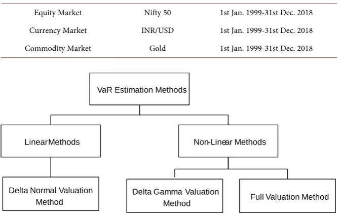
3.1. Data PeriodThe study investigates three markets: equity, currency and commodity for a pe-riod of 20 years so as to incorporate different economic conditions. There are a total of 4981, 5281 and 5081 observations for Nifty 50 returns, INR/USD returns and gold returns respectively (Table 1).
The daily close price for each of the asset is considered as the input to the various models. The close prices are then converted into lognormal returns us-ing the followus-ing equation:
(
1)
100R=l Rt Rt− ×
where,
R = Return of the closing prices. Rt= Today’s closing prices.
Rt − 1= Previous day’s closing prices. Ln = log normal.
3.2. Sources of Data
The secondary sources of data used in this study are obtained from NSE, BSE, RBI and Bloomberg database amongst others.
3.3. Various Approaches for Estimating VaR
DOI: 10.4236/tel.2019.98177 2829 Theoretical Economics Letters Table 1. Data period for the study.
Equity Market Nifty 50 1st Jan. 1999-31st Dec. 2018 Currency Market INR/USD 1st Jan. 1999-31st Dec. 2018 Commodity Market Gold 1st Jan. 1999-31st Dec. 2018
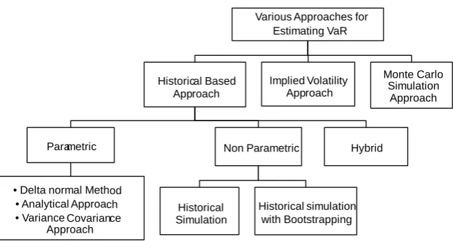
Figure 1. VaR estimation methodologies classification I. (Source: Author Generated).
The Delta Normal Valuation Method is to be used in case of linear derivative such as forwards, Futures and swaps.
The Delta Gamma Valuation Method is to be used in case of non-linear de-rivatives which are well behaved like options and non-option embedded bonds.
The Full Revaluation Method is to be used in case of non-linear misbehaved series like option embedded bonds i.e. callable bonds or puttable bonds and for structured products like Mortgage Backed Securities (MBS). It is also to be used when there exist cross partial effects (Figure 2).
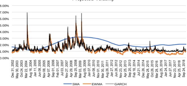
The second type of classification is based on the type of data used for calculating VaR. Historical based approaches use historical data to calculate the volatility for VaR while the implied volatility approach uses option price and Black and Scholes Model (BSM) to back calculate the forward looking implied volatility.
3.3.1. Parametric Approaches
Parametric Approaches are based on the assumption that the asset returns follow a certain distribution, say normal distribution. It is also known as Delta Normal Method, Analytical Approach or Variance Co-Variance (VCV) Approach.
1) Why volatility is required for calculating VaR:
Suppose we have a portfolio whose returns are normally distributed with a daily mean = 0 and daily volatility = 1.5%. The portfolio is currently worth $1000 million. The 1-day VaR at 99% confidence interval is as follows:
For an area of 1 % in a tail z = 2.33. VaR (%) = z *σ = 2.33 * 1.5% = 3.5%.
VaR (in $ terms) = 3.5% of $1000 million = $ 35 million.
Thus, maximum possible loss that can take place in a day is $ 35 million with 99% confidence i.e. with just 1% chance of being exceeded. In 1% of the worst cases, loss would be at least $ 35 million.
VaR Estimation Methods
Linear Methods
Delta Normal Valuation Method
Non-Linear Methods
Delta Gamma Valuation
DOI: 10.4236/tel.2019.98177 2830 Theoretical Economics Letters Figure 2. VaR estimation methodologies classification II. (Source: Author Generated.)
The above example goes to show that the standard deviation is a necessary input for estimating the Value at Risk.
2) Observed properties of volatility
A volatility estimation engine must capture the following three properties of volatility:
a) Adaptability: Volatility is dynamic or regime switching so the engine should keep on forecasting new volatility based on innovation.
b) Persistence: Volatility is persistent or sticky, i.e. it tends to cluster around the current value.
c) Mean Reverting: Volatility tends to revert back to a particular mean rever-sion level.
3) Parameter Estimation (MLE) and choice of window size Parameter Estimation Techniques
The technique is designed in such a manner that we try to maximize the probability of the observations occurring. The Maximum Likelihood Estimation technique is used in the study for parameter calibration of the various probabili-ty distributions considered in the VaR models.
Choice of window size
There is a trade off between statistical accuracy i.e. precision and adaptability when selecting a window size for a volatility estimation engine.
The study uses 1000 days window size to incorporate persistency. The VaR is estimated using approximately past 4 years data.
4) Method 1: VaR using SMA
The simple moving average is also known as the historical standard deviation approach. The unbiased formula for calculation variance under the SMA ap-proach is as follows:
2 2 k
σ =
∑
µwhere, μ = Past Returns k-window size. 5) Method 2: VaR using EWMA
Various Approaches for Estimating VaR
Historical Based roach App
Parametric
• Delta normal Method • Analytical Approach • Variance Covariance
Approach
Non Parametric
Historical Simulation
Historical simulation with Bootstrapping
Hybrid Volatility Implied
Approach
Monte Carlo Simulation
DOI: 10.4236/tel.2019.98177 2831 Theoretical Economics Letters Variance under EWMA (Exponential weighted moving average) is given by the following equation:
(
)
2 * 2 1 1 * 2 1
n n n
σ =λ σ − + −λ µ −
where, μ = Past Returns. λ = Decay Factor.
The beauty of EWMA is the requirement of less storage. We just need to store the previous day’s estimate of volatility i.e. σn−1 and the recent innovation σn−1.
The RiskMetrics approach is just an EWMA model that uses a pre-specified decay factor for daily data, which is equal to 0.94 and a factor equal to 0.97 for monthly data.
6) Method 3: VaR using GARCH
One of the most popular methods of estimating volatility is the generalized autoregressive conditional heteroskedastic (GARCH) (1,1) model. The best way to describe GARCH (1,1) model is to take a look at the formula:
2 2 2
1 1
n n n
σ = +ω αµ − +βσ −
where:
α = weight on the previous period’s return β = weight on the previous volatil-ity estimate ω = weighted long-run variance = ƔVL.
VL = long-run average variance = ω/(1 – α − β)α+ β + Ɣ = 1α + β < 1 for sta-bility so that Ɣ is not negative.
If α + β > 1 then Ɣ < 0, then GARCH model becomes unstable, as the variance becomes mean fleeing then compared to mean reverting.
7) Analogy between EWMA with GARCH
EWMA (Exponential weighted moving average) is a special case of GARCH when α + β = 1.
Conceptually GARCH is better than EWMA as it captures mean reverting tendency, which EWMA approach doesn’t.
EWMA is considered better than GARCH, as it is parsimonious. Requires just one parameter estimation i.e. λ. Whereas GARCH requires three para-meters α, β and ω.
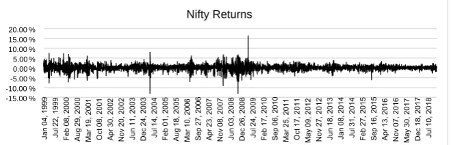
However, empirically it was found that GARCH performed better than EWMA for each asset class under consideration (Figure 3).3.3.2. Non Parametric Approaches
1) Historical Simulation
Historical Simulation does not assume any particular distribution. It also does not suffer from the problem of fat tails as it considers the extreme values of the returns as well.
The following steps were performed to estimate VaR under HS approach: Step 1: Collected past returns of each asset class.
Step 2: Arranged them from worst to best.
DOI: 10.4236/tel.2019.98177 2832 Theoretical Economics Letters Figure 3. Comparison of the three volatility estimation engines. (Source: Author Gener-ated).
2) Historical Simulation with Bootstrapping
Historical Simulation with Bootstrapping is an improved approach of Historical Simulation approach. It involves random sampling from past observa-tions with replacement. We then arrange the data from worst to best. To get the VaR, we slice the significance level percentage from the worst side.
4. Analysis and Findings
This study employs both numerical measures and graphical measures to evaluate the predictive ability of the VaR models as stated in the previous section. Mul-tiple analytical techniques as mentioned in the figure below may be employed (Figure 4).
4.1. Descriptive Analysis
Descriptive analysis involves describing the characteristics of data i.e. summa-rising the data.
a) Numerical Measures (Table 2) b) Graphical Measures:
The figure (Figure 5) reflects daily Nifty 50 Index from 1st Jan 1999 to 31st Dec
2018. The horizontal axis corresponds to time while the vertical axis displays the value of the index.
Nifty 50 log returns reflect a subdued volatility over 20 years. The stationarity and volatility clustering in the market is evident (Figure 6).
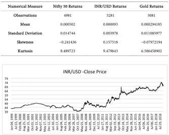
The above figure (Figure 7) portrays the daily INR/USD from 1st Jan 1999 to
31st Dec 2018. The horizontal axis corresponds to time while the vertical axis
displays the closing exchange rate.
The above figure reflects the INR/USD log returns. The stationarity and vola-tility clustering in the market is visible (Figure 8).
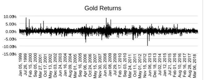
The daily gold close price from 1st Jan 1999 to 31st Dec 2018 is chalked in the
figure above (Figure 9). The horizontal axis corresponds to time while the ver-tical axis displays gold close price.
% 0.00 1.00% 2.00% % 3.00
% 4.00
% 5.00
% 6.00
% 7.00
% 8.00
Projected Volatility
DOI: 10.4236/tel.2019.98177 2833 Theoretical Economics Letters Figure 4. Data Analysis techniques for VaR Model prediction (Source: Au-thor Generated).
Figure 5. Nifty 50 historical data (Source: Author Generated).
Figure 6. Nifty 50 Log returns (Source: Author Generated).
Even ingold returns, the stationarity and volatility clustering in the market areee visible (Figure 10).
4.2. Unit Root Analysis
Unit root analysis is tested using the Augmented Dickey-Fuller (ADF) test. To test for stationary, we conducted the ADF test. It is used for larger and more complicated set of time series models. We can perform GARCH forecasting only on stationary data. Thus, the data needs to be made stationary.
riptive Desc
istics Stat
erical Num
sures Mea
Measure of Central Tendency
Measure of Dispersion
Measure of Skewness
Measure of Peakedness
Graphical Measures
Histogram Leaf Plot Box plot Inferential
St atistics Data Analysis
0 2000 4000 6000 8000 10000 12000 14000
Nifty -Close Price
% -15.00
% -10.00
% -5.00
0.00 % % 5.00
% 10.00
% 15.00 20.00 %
[image:10.595.209.539.463.569.2]DOI: 10.4236/tel.2019.98177 2834 Theoretical Economics Letters Table 2. Numerical measures (Consolidated).
Numerical Measure Nifty 50 Returns INR/USD Returns Gold Returns Observations 4981 5281 5081
[image:11.595.204.541.388.522.2]Mean 0.000502 0.000093 0.000294185 Standard Deviation 0.014744 0.003978 0.011085977 Skewness −0.241436 0.157518 −0.07972194 Kurtosis 8.489723 9.479643 6.586458902
[image:11.595.209.537.564.702.2]Figure 7. INR/USD historical data (Source: Author Generated).
Figure 8. INR/USD Log returns (Source: Author Generated).
Figure 9. Commoditized Gold historical data (Source: Author Generated).
39 44 49 54 59 64 69 74 79
INR/USD -Close Price
% -3.50
% -2.50
% -1.50
% -0.50
% 0.50
% 1.50
% 2.50 3.50%
INR/USD Returns
0 200 400 600 800 1000 1200 1400 1600 1800 2000
DOI: 10.4236/tel.2019.98177 2835 Theoretical Economics Letters Figure 10. Commoditized Gold log returns (Source: Author Generated).
When having a unit root ρ1 = 1 in the following equation
1 1 2 1 3 2
Yt=ρ Y t− +ρ ∆ − +Yt ρ ∆ − +Yt εt
This is called the augmented Dickey-Fuller (ADF) test and implemented in many statistical and econometric software packages. We have conducted ADF test on Excel through Real Stat software package.
4.3. Back-Testing Results with Exceedances
Back testing is the process of comparing losses predicted by the value at risk (VaR) model to those actually experienced over the sample testing period.
If a model were completely accurate, we would expect VaR to be exceeded (also called as an exception) with the same frequency predicted by the confi-dence level used in the VaR model. In other words, the probability of observing a loss amount greater than VaR is equal to the significance level.
When using the above back testing approach, the following three desirable attributes of VaR estimates are to be evaluated: VaR estimate should be un-biased, adaptable and robust.
5. Conclusions
5.1. Inferences
The results show that parametric model using normal distribution with GARCH (1,1) fits best for estimating value at risk at 99% confidence interval in all the three markets under consideration.
The research indicates that the Historical simulation model with 99% confi-dence fails the backtesting test for each asset class.5.2. Implications
The findings will assist the commercial and investment banks in determining the extent and occurrence ratio of potential losses in their institutional port-folios.
The study will help build additional confidence in measuring the extent of
potential forced reductions of the firm’s capital over short time periods. %
-15.00 % -10.00
% -5.00
% 0.00
% 5.00
% 10.00
DOI: 10.4236/tel.2019.98177 2836 Theoretical Economics Letters
5.3. Limitations
The statistical probability distributions assumed for testing purposes are li-mited to normal and student-t distributions only.
The calculations done are to estimate only 1-day VaR. However, the study can be extended to estimate 30-day VaR, 50-day VaR, 100 day-VaR accord-ing to the investors’ need and risk exposure.
The research studies only the market risk in the Indian markets. The VaR concept can be applied to estimate the credit risk, operational risk and li-quidity risk.
The rolling window size considered for backtesting is of 1000 days. Rolling window sizes play a crucial role in determining the VaR as it leads to a choice between persistence and adaptability.
The study considers three markets viz. index, exchange rate and commodi-ties. The models can be used for individual stocks as well for derivative in-struments like futures and options.Conflicts of Interest
The authors declare no conflicts of interest regarding the publication of this paper.
References
[1] Kuester, K. (2006) Value-at-Risk Prediction: A Comparison of Alternative Strate-gies. Journal of Financial Econometrics, 4, 53-89.
https://doi.org/10.1093/jjfinec/nbj002
[2] Skoglund, J., Erdman, D. and Chen, W. (2010) The Performance of Value-at-Risk Models during the Crisis. The Journal of Risk Model Validation, 4, 3-21.
https://doi.org/10.21314/JRMV.2010.052
[3] Chen, L., Peng, J., Zhang, B. and Rosyida, I. (2017) Diversified Models for Portfolio Selection Based on Uncertain Semivariance. International Journal of Systems
Science, 48, 637-648. https://doi.org/10.1080/00207721.2016.1206985
[4] Zhang, B., Peng, J. and Li, S. (2015) Uncertain Programming Models for Portfolio Selection with Uncertain Returns. International Journal of Systems Science, 46, 2510-2519. https://doi.org/10.1080/00207721.2013.871366
[5] Koutsoyiannis, A. (2006) A Short-Run Pricing Model for a Speculative Asset, Tested with Data from the Gold Bullion Market. Applied Economics, 15, 563-581. https://doi.org/10.1080/00036848300000037
[6] Gupta, S., Choudhary, H. and Agarwal, D.R. (2018) An Empirical Analysis of Mar-ket Efficiency and Price Discovery in Indian Commodity MarMar-ket. Global Business
Review, 19, 771-789. https://doi.org/10.1177/0972150917713882
[7] Gencay, R. and Selçuk, F. (2004) Extreme Value Theory and Value-at-Risk: Relative Performance in Emerging Markets. International Journal of Forecasting, 20, 287-303. https://doi.org/10.1016/j.ijforecast.2003.09.005
DOI: 10.4236/tel.2019.98177 2837 Theoretical Economics Letters Estimation: Evidence from Turkey. The Journal of Risk Finance, 11, 164-179. https://doi.org/10.1108/15265941011025189
[10] Timotheos, A. (2010) Idiosyncratic Risk in Emerging Markets. Financial Review, 45, 1053-1078. https://doi.org/10.1111/j.1540-6288.2010.00285.x
[11] Lehar, A., Scheicher, M. and Schittenkopf, C. (2002) GARCH vs. Stochastic Volatil-ity: Option Pricing and Risk Management. Journal of Banking & Finance, 26, 323-345. https://doi.org/10.1016/S0378-4266(01)00225-4
[12] Walsh, D.M. and Tsou, G.Y.-G. (1998) Forecasting Index Volatility: Sampling In-terval and Non-Trading Effects. Applied Financial Economics, 8, 477-485. https://doi.org/10.1080/096031098332772
[13] Yu, J. (2002) Forecasting Volatility in the New Zealand Stock Market. Applied
Fi-nancial Economics, 12, 193-202. https://doi.org/10.1080/09603100110090118
[14] Angelidis, T., Benos, A. and Degiannakis, S. (2003) The Use of GARCH Models in VaR Estimation. Statistical Methodology, 1, 105-128.
https://doi.org/10.1016/j.stamet.2004.08.004
[15] Rockafellar, R. and Uryasev, S. (2002) Conditional Value-at-Risk for General Loss Distributions. Journal of Banking & Finance, 26, 1443-1471.
DOI: 10.4236/tel.2019.98177 2838 Theoretical Economics Letters
Appendix
Rolling EWMA code in R language:
library ("tseries") library ("zoo") library ("forecast") library ("FinTS") library ("rugarch")
Niftydata <- read.csv ("Nifty4981.csv") attach (Niftydata) Nifty.return <- Return result = matrix (c (0,0,0,0), ncol = 4) a = 1 while (a < 3982)
{b=a+999
X<- Nifty.return[a:b] ewma_spec <- ugarchspec (variance.model = list (model = "iGARCH", garchOrder = c (1,1)), mean.model = list (armaOrder = c (0,0), include.mean = TRUE), distribution.model = "norm", fixed.pars = list (omega = 0)) ewma_fit<- ugarchfit (spec = ewma_spec, data = X)
result = rbind (result,ewma_fit@fit$coef) a=a+1 } write.csv (result,"result.csv")
Rolling GARCH (1,1) code in R language
library ("tseries") library ("zoo") library ("forecast") library ("FinTS") library ("rugarch") Niftydata<- read.csv ("Nifty4981.csv") attach (Niftydata) Nifty.return <-Return result = matrix (c (0,0,0,0,0,0), ncol = 6) a = 1 while (a < 3982)
{b = a + 999
X<- Nifty.return[a:b]
res_garch11_spec <- ugarchspec (variance.model = list (garchOrder = c (1,1)), mean.model = list (armaOrder = c (1,1))) res_garch11_fit <- ugarchfit (spec = res_garch11_spec, data = X) result = rbind (result, res_garch11_fit@fit$coef) a = a+1