TVE 16 045 juni
Examensarbete 15 hp
Juni 2016
Integrated Thermal Energy Systems
A Case Study of Nya Studenternas IP and
Uppsala University Hospital
Mika Bäckelie
Thomas Lindén
Freja Nielsen
Emma Pålsson
Teknisk- naturvetenskaplig fakultet UTH-enheten Besöksadress: Ångströmlaboratoriet Lägerhyddsvägen 1 Hus 4, Plan 0 Postadress: Box 536 751 21 Uppsala Telefon: 018 – 471 30 03 Telefax: 018 – 471 30 00 Hemsida: http://www.teknat.uu.se/student
Abstract
Integrated Thermal Energy Systems
Mika Bäckelie, Thomas Lindén, Freja Nielsen, and Emma Pålsson
The aim of this project is to evaluate the possibility to integrate, in terms of energy, the future Nya Studenternas IP and Uppsala University Hospital. The focus is on integration of thermal energy solutions. To cover the cooling demand a seasonal snow storage and the use of cooling machines is studied. For the heat demand a joint heat storage is investigated which is heated partly with the excess heat from cooling machines. The
environmental impact in terms of CO2 emissions is investigated.
A conclusion drawn from the project is that the use of district heating and cooling of Nya Studenternas IP and the Uppsala University Hospital could be reduced in several ways by integrating the energy systems of the two facilities. For instance, with the
support of a seasonal snow storage and cooling machines for cooling, and heat obtained from the cooling machines for heating, the emissions of CO2 could be reduced with 36% based on a Nordic electricity mixture. Out of the suggested integrated energy solutions the most efficient when it comes to reducing CO2 emissions is cooling and heating through cooling machines with a capacity of reducing the CO2 emissions of 20.6 %.
ISSN: 1650-8319, TVE 16 045 juni Examinator: Joakim Widén Ämnesgranskare: Magnus Åberg
Table of contents
Table of contents ... 0
1. Introduction ... 2
1.1 Aim and research questions ... 3
1.2 Delimitations ... 3
2. Background ... 4
2.1 Uppsala University Hospital... 4
2.2 Nya Studenternas IP ... 4
2.3 Energy solutions to be integrated ... 5
2.3.1 District heating ... 5
2.3.2 District cooling ... 5
2.3.3 Seasonal snow storage ... 5
2.3.4 Cooling machines... 7
2.3.5 Solar collectors for heat ... 8
2.3.6 Heat storage ... 9
3. Methodology and Data ... 10
3.1 Data of Uppsala University Hospital ... 10
3.2 Model of Nya Studenternas IP ... 11
3.3 Environmental impact ... 14
3.3.1 Emissions from district heating and cooling ... 14
3.3.2 Emissions from electricity production ... 15
3.3.3 Emissions from different thermal energy sources ... 16
3.4 Seasonal snow storage ... 16
3.5 Cooling Machines ... 21
3.5.1 Winter season ... 21
3.5.2 Summer season ... 24
3.5.3 Total annual production ... 24
3.6 Hot water storage ... 25
4. Results ... 32
4.1 Snow storage ... 32
4.2 Cooling machines ... 33
4.3 Snow storage and cooling machine integration ... 36
4.4 Hot water storage ... 37
4.5 Results summary ... 39
5. Sensitivity Analysis ... 40
1
5.2 Hot water storage ... 42
6. Discussion ... 44
7. Conclusions ... 46
2
1. Introduction
"This is not a partisan debate; it is a human one. Clean air and water, and a livable climate are inalienable human rights. And solving this crisis is not a question of politics. It is our moral obligation." - Leonardo DiCaprio, 2016.
DiCaprio, a very influential actor and environmental advocate, is just one of many prominent people to declare the importance of a sustainable development. In accordance with the Brundtland commission such a development is defined as a development that “meets the needs of the present without compromising the ability of future generations to meet their own need” (United Nations 1987, p. 41). Due to conventional methods of energy extraction, with corresponding impacts on the environment, our climate is reaching a critical status. With a continuously increasing population and welfare come an unavoidable and necessary increase in the consumption of energy (International Energy Agency 2015, p. 20, 33). This leaves us with a responsibility to find ways in which these needs can be met without causing continuously increasing environmental damage.
In order to meet today’s energy demands every detail of the distribution chain must be taken into consideration. The importance of finding new solutions for an increasing energy demand has never been greater. These solutions include both finding new energy sources as well as utilizing untapped resources. Such a holistic perspective includes issues like possible use of excess energy capacity, which is most commonly existing in the form of thermal energy. Bearing this in mind, modern construction projects can be planned in ways to avoid loss of excess energy, either by internal recycling or by distribution to another user. For example, public buildings with heat generating activities and large energy demands, could be linked together in an integrated energy system.
Integrated energy systems between buildings is however only of interest if achieved with effectiveness and a minimal damaging impact on the environment. Possible integrations are highly dependent on the local conditions, energy demands and the activities from which thermal energy might be obtained. In order to establish such an energy exchange the factors must be mapped.
A project currently facing the challenges of energy demand, local conditions and the question of where thermal energy might be obtained is the construction of Nya Studenternas IP, a sports arena planned to be located in central Uppsala. During the development of this new facility there has been a discussion about whether it would be possible to create a systematic energy integration with the nearby hospital, Uppsala University Hospital. This dialogue includes the integration of potential energy sources to maximize energy efficiency. The goal is to achieve a sustainable solution which is mutually beneficial for all actors involved.
3
1.1 Aim and research questions
The aim of this report is to investigate the possibilities to create thermal energy system integrations for Uppsala University Hospital and Nya Studenternas IP, and to find sustainable solutions that are energy efficient. The energy solutions will be examined in reference to a full use of district heating and cooling.
In order to meet the objectives these research questions are to be answered
● What are the seasonal thermal energy demands for the future Nya Studenternas IP and what are the total thermal energy demands for Nya Studenternas IP and Uppsala University Hospital?
● To what extent could alternative energy solutions to district heating and cooling, such as heat and cold storage and increased utilization of available thermal capacity, cover these demands?
● In terms of emissions, how will alternative and complementary energy solutions to district heating and cooling affect environmental impact?
1.2 Delimitations
This project will focus on the implementation of integrating thermal energy systems and not take into account any exchange of electricity. This because the CO2 emissions from
production of thermal energy supply in the form of district heating and cooling contributes to the local pollution, which is not the case for the electricity consumed. This project will not present detailed plans or schemes, but rather offer an overall description of different possible solutions.
The possible solutions presented focus mostly on cooling and are therefore modeled to suit the cooling demand. Some solutions may partially cover the heating demand as well but in such cases, the available heat will be the excess heat generated in a cooling process. The only exception to this rule is heat generating solar collectors.
Only the emissions from operational use and not emissions from construction will be looked at. Environmental impact will be presented as CO2 emissions and compared to
the impact of current energy solutions. These calculations are based solely on emissions due to electricity and thermal energy consumption. No financial analysis for the
4
2. Background
In this section the two areas Uppsala University Hospital and Nya Studenternas IP will be presented. A description of the existing thermal energy system at the hospital as well as the different options for an integrated energy system including Uppsala University Hospital and the future sports arena will follow. Integrated solutions with seasonal snow storage, cooling machines, and heat storage will be described. District cooling and heating systems in Uppsala will be briefly presented.
2.1 Uppsala University Hospital
Uppsala University Hospital is a teaching hospital from 1867 but dates all the way back to the 14th century (Akademiska sjukhuset (a) 2016). The hospital consists of a
complex of buildings which covers almost all medical departments. The hospital includes operating theatres, laboratories and provides a major part of the medical education and nurse training in association with Uppsala University (Akademiska sjukhuset (b) 2016). The hospital has about 8 000 employees and the capacity of 943 hospital beds and each year over 30 000 operations are conducted (Akademiska sjukhuset (c) 2016).
In 2013 major renovations started. The project is called Future of Akademiska and is one of the largest redevelopments of Uppsala University Hospital. By 2020, rebuildings, upgrades, and a new care and treatment building is to be built. The rebuilding started due to that many 40 years old buildings were in need of renovation, but also due to increased regulatory requirements such as fire safety, sanitary facilities and working environment (Akademiska sjukhuset (d) 2016).
Uppsala University Hospital has a large demand of thermal energy. Sterile
environments and working facilities requires both high standard and reliable supply of comfort heating and cooling. Today the thermal energy is supplied by district heating and cooling by the local district heating system operated by Vattenfall. Heat generated through different processes in the hospital are being recycled internally and used for comfort heating, and when the outside-temperature air allows it, free cooling is used to cool the indoor air (Larsson, 2016).
2.2 Nya Studenternas IP
In 2017 a major reconstruction of the sports stadium Studenternas IP will commence, a project led by Sportfastigheter. It is supposed to result in a whole new soccer arena with capacity for 8 000-10 000 spectators. Adjacent to the arena a multi-story facility
(referred to as the F-house), of about 10 000 m2 will be built, including restaurants,
locker rooms, VIP-lounge, and offices (Sportfastigheter, 2016).
In addition to the soccer field there are two, currently existing, ice fields which are used from mid-October to mid-March. When the outdoor temperature is above -5 degree
5
Celsius the ice fields are maintained with cooling from cooling machines. The cooling machines that are currently being used to cool the ice fields were installed in 1958. In addition to the reconstruction of the arena, new cooling machines will also be installed with a peak effect of 2 800 kW (Lindberg, 2016).
The thermal energy supply to Nya Studenternas IP will mainly consist of district heating and cooling delivered by Uppsala district heating system operated by Vattenfall. As for the heating, there are plans to use the excess heat generated by the cooling machines for warm water and comfort heating. During the warmer periods, usually ranging from May to late August, comfort cooling will be supplied to office- and process areas through district cooling. Methods of free cooling are being evaluated, along with the possible use of a seasonal snow storage. Plans to add solar panels to some of the rooftops are being discussed, this to possibly cover parts of the electricity demand (Lindberg, 2016).
2.3 Energy solutions to be integrated
2.3.1 District heating
District heating is a closed system of insulated pipes through which heated water from a heat plant is supplied to the heat users in the system. The temperature of the water leaving the heat plant varies between 70 and 120 degrees Celsius depending on season and system. The water is then used for space heating mainly through radiators and water heating. District heating is delivered to about 50 percent of Swedish buildings (Svensk Fjärrvärme (a), 2016).
District heating often utilize heat that would otherwise be wasted, many times waste from forestry, excess heat from industries, peat, or waste from households. Many heat plants use a combination of different energy sources. In Uppsala heat is mainly generated in waste incineration plants. Incineration is a part of the Swedish waste management treatment (Svensk Fjärrvärme (a), 2016).
2.3.2 District cooling
There are different methods of producing district cooling. One of them being absorption cooling, which is the most common in Uppsala heat and cooling plant. Absorption cooling utilizes the production of the thermal energy for district heating. By increasing the pressure, the water evaporates at a temperature of about three degrees Celsius. The water is then distributed in the district cooling system all over Uppsala (Svensk
Fjärrvärme (b), 2016).
2.3.3 Seasonal snow storage
The method of using chilled surroundings to store and preserve cool material is an ancient strategy. Snow, caverns, lakes, and low temperature air are a few sources that could offer cooling potential. Free cooling is the modern term used to describe cooling
6
that is naturally obtained from chilled surroundings rather than using mechanical refrigeration. Generally, free cooling is low temperature energy extraction that only requires a pump or a fan to utilize the cold (Skogsberg, 2005).
One method of free cooling is using seasonal snow storage. Snow or ice is either
collected or created artificially during the winter and then stored until summer, when the cold is utilized. Snow can be stored in ponds, underground, on ground, or indoors. A common nominator for these different storing methods is that insulation is required to slow down the melting process. Storage indoors is done with a thermally insulated storehouse. Underground storage in caverns do not need any extra insulation. A snow depot on ground or in a pond requires insulation, often being a layer of wood chips, which has in recent studies proved to be an efficient snow insulator (Skogsberg, 2005). The process of extracting cold from snow uses a chilled carrier which passes through the stored snow and then transfer the carrier to a load. The carrier then absorbs heat from the load resulting in a cooler environment. The cold carrier is then transported back to the snow storage and the process can be repeated. Since heat is transferred spontaneously from hot to cold environments, the snow storage will absorb heat from the cold carrier, resulting in the snow melting. Snow melting due to cold extraction is defined as forced melting. Natural melting is heat transfer from external sources to the snow storage. The amount of natural melting can vary a lot depending on geometric structure of the storage as well as annual levels of temperature and precipitation. However, a large snow storage with at least 0.2 dm of wood chip insulation loses approximately 30-35% of its volume because of natural melting (Näslund 2012, p. 12). The Sundsvall Regional Hospital is the only large scale operational seasonal snow storage system in Sweden, see figure 1. With an annual cooling demand of around 1000 MWh, up to 90 % is supplied through snow cooling (Granström et al. 2010, p. 4). With a slightly inclined (~1%) open pond the snow storage is designed for a maximum capacity of 60000 m3. A 0.1 m layer of wood chips is used for insulation, resulting in a
snow perseverance that lasts the summer.
Technically, cooling energy is obtained by pumping melted snow from the snow storage through heat exchangers connected to the cooling system within the hospital. The water is cleaned through filters, collecting all the toxic emissions from the snow. Two pumps provide a water flow with the rate of 0.035 respectively 0.050 m3/s flow through the
heat exchangers, with an effect of 1 000 respectively 2 000 kW. After the melted water is heated by the hospital through the heat exchangers, the water is recirculated to the snow, repeating the process (Skogberg, 2005).
7
Figure 1 Illustration of the Sundsvall Hospital snow cooling system.
2.3.4 Cooling machines
When it is not possible to cool ice fields with the outside-temperature air by free cooling, one method is to create artificially frozen ice by using a cooling machine. Due to that the second law of thermodynamics prohibits heat to be transferred from a cold to warm environment without any input work, the machine is designed to move thermal energy opposite to the direction of spontaneous heat flow by using external power. It absorbs the thermal energy from a colder medium, a heat source, and releases it to a warmer medium, a heat sink.
The machine is also called a heat pump and consists of four main parts: an evaporator, a compressor, a condenser and an expansion valve. The machine uses a refrigerant as an intermediate, which evaporates when it absorbs the heat in the evaporator. The
refrigerant then runs through the compressor which uses electricity to compress the refrigerant, causing it to rise in temperature. The vaporized and compressed refrigerant then transports the absorbed heat and releases it in the condenser, where the refrigerant condenses. The refrigerant then runs through the expansion valve, causing an expansion and the temperature decreases. The refrigerant then again evaporates in the evaporator and the process is restarted (Britannica Academic 2016).
When artificially frozen ice is created, water on a field is working as an evaporator. The refrigerant absorbs thermal energy from the water, causing the water to drop in
temperature and eventually freeze to ice. On the condenser side the outdoor air is used to condense the refrigerant. By using fans, the condensing process could be done more efficiently, but the absorbed heat is just released outside in the air. This heat is often of low-grade, approximately 20-40°C, but the amount of heat delivered is high (Svensk Fjärrvärme (b) 2009). By taking care of this heat instead of just releasing it outside, the
8
cooling machine could be used more efficiently. In figure 2 a cooling machine at an ice rink is shown.
A measurement for how efficiently a cooling machine operates is determined by its Coefficient of Performance, COP. The COP is an evaluation of how much cooling or heating capacity is produced per unit of input work. COPheating is always 1 unit higher
than COPcooling, meaning that the amount of heat obtained from cooling machines will
be higher than the amount of cooling. If a cooling machine operates with the cooling capacity of COPcooling around 3, then 3 times the effect of input work will be obtained as
cooling. The same cooling machine will in the same process also generate 4 times the amount of the input work as heat. (Thermia [no date])
Figure 2 Illustrative principle of ice rink cooling (Wwip 2003).
2.3.5 Solar collectors for heat
The sun provides the Earth with massive amounts of energy through its radiation. The use of solar collectors as support to the heating system is a feature commonly seen in modern buildings. They are equipped with a coating which absorbs short wave solar radiation and converts it into long wave heat rays. In the front of the coating is a protective glass and insulation on the back. The glass is designed to allow most of the short wave sunlight to pass through. It does cause an optical loss, corresponding to the percentage of energy that failed to pass through. Solar collectors also have a thermal loss since some of the heat is emitted. On average, the solar collectors have an optical efficiency, percentage of energy from solar rays that passes through the protective glass, of about 70-80%. The thermal efficiency varies with the season (Solarserver, 2011). To be able to save solar heat for later use solar collectors are often connected to a heat storage. It is common practice to use solar collectors as an external source of thermal energy for hot water storages. The water in the hot water storage is heated by the collectors when the sun is shining and can maintain its temperature for some time without contribution from solar heat (Solarserver, 2011).
9
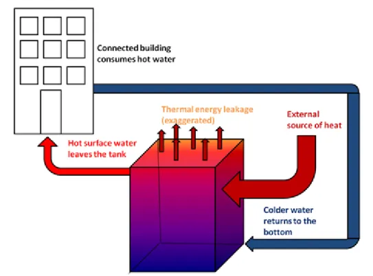
2.3.6 Heat storage
One conventional method of seasonal heat storage is to store heat in water. Due to its high specific heat capacity, water has an excellent ability of keeping its change in temperature at a low rate. When excess heat is available the water is heated. Since its temperature drops very slowly the water will remain warm until the outdoor temperature gets low enough to cause a need for extra heat. This heat can then be derived from the water (Svensk Fjärrvärme, 2008).
The use of water as a mean of seasonal heat storage calls for a large-scale container designed to maintain the water temperature, much the same as a big thermos. Hot water storage tanks are usually made of insulating material to prevent heat exchange between the water and its surroundings (Svensk Fjärrvärme, 2008).
Figure 3 Illustration of hot water storage tank.
Any source of thermal energy can be used to heat the water in the storage tank. It is however common to connect it to solar collectors, seen as external source of heat in figure 3. This since the solar collectors tend to generate heat when the demand for heat is low and it is desirable to store the heat for future use (Svensk Fjärrvärme, 2008).
10
3. Methodology and Data
The model of the integrated energy systems of Nya Studenternas IP and Uppsala
University Hospital is presented in figure 4. The model of the different energy solutions will be described as well as the data collected. The gathering of information has mainly been done by interviews and e-mail contact as well as literature studies.
Figure 4 Suggested energy solutions would be connected to Uppsala University Hospital, Nya Studenternas IP and to each other. It marks the demands for heating and cooling and their complementary energy solutions. The energy solutions with light grey
lines are the ones that will be presented in the modelling. Arrows in dark red for heating and light blue for cooling indicates thermal energy exchange.
3.1 Data of Uppsala University Hospital
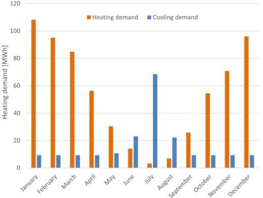
The data for the heating and cooling energy demands for Uppsala University Hospital was obtained from Uppsala County Council Service. The data was based on use of district heating and cooling the last two years. The representation of Uppsala University Hospital in this report will only include the thermal demands of currently existing and operational buildings. The energy use is presented in figure 5 for both heating and cooling for each month. The thermal energy demands of Uppsala University Hospital are assumed to be annually constant based on the use of district heating through 2014-2015. Similarly for district cooling through 2010 to 2014-2015.
11
Figure 5 Heating and cooling demand at Uppsala University hospital.
3.2 Model of Nya Studenternas IP
Estimated data was provided for the future Nya Studenternas IP, by Sportfastigheter. In order to determine the monthly basis of thermal energy demands, MATLAB was used and the result of these calculations is presented in figure 6. The simulation of monthly thermal energy use was based on outside temperatures provided by Swedish
Meteorological and Hydrological Institute together with an estimation of annual thermal demand from Sportfastigheter. The model includes simulations of both heating and cooling demands. To create reliable monthly demands of cooling during the summer period of April to end of September, daily average weather data was used from 2005 - 2015. The model for cooling consists of two types of cooling demands; comfort- and process cooling. For comfort cooling, the script calculates the number of cooling degree days each month. If the average temperature is higher than a reference temperature, the difference is added to the number of degree days. The reference temperature is a variable that can be changed, which makes it possible to regulate when cooling is needed based on the outdoor temperature. The comfort cooling demand is then divided on a monthly basis according to the number of cooling degree days during the months, by using the preliminary energy demand for cooling.
Process cooling for office buildings was modeled by using preliminary rated power of the cooling processes given by Sportfastigheter. By assuming that the cooling processes operates at rated power the whole year, a roughly estimated energy demand is obtained. The demand is assumed to be evenly distributed over the year since the process cooling is not believed to be as dependent on the outdoor temperature as the comfort cooling is.
0 2000 4000 6000 8000 10000 12000 H eat in g d em an d [MWh ]
12
Figure 6 Modeled heating and cooling demand at Nya Studenternas IP.
The model of heating demand is based on the average number of degree days for each month the last two years. The degree days that were used were obtained from Uppsala County Council Service. By using the preliminary energy demand for comfort heating and hot water over a year, which was obtained from Sportfastigheter, the energy is divided on a monthly basis according to the number of heating degree days during the months. Figure 7 shows the total heating demand at Nya Studenternas IP and Uppsala University Hospital and figure 8 shows the total cooling demand.
0 20 40 60 80 100 120 H eat in g d em an d [MWh ]
13
Figure 7 The total heating demand of Nya Studenternas IP and Uppsala University hospital.
Figure 8 The total cooling demand of Nya Studenternas IP and Uppsala University hospital. 0 2000 4000 6000 8000 10000 12000 H eat in g d em an d [MWh ]
Uppsala University Hospital Nya Studenternas
0 500 1000 1500 2000 2500 H eat in g d em an d [MWh ]
14
3.3 Environmental impact
The new integrated energy solutions will affect the environment in different ways. To compare their sustainability, one possibility is to investigate the CO2 emissions of the
solutions and how it will vary. CO2 is one of the greenhouse gases that has the biggest
impact on the climate, making it of interest to examine. In this project the emissions from producing district heating and cooling will be used as reference. The new solutions will only consume electricity when operating. Consequently, there will be of interest to compare the emissions from district heating and electricity production and see if there has been any decrease of emissions of CO2 with the new solutions.
3.3.1 Emissions from district heating and cooling
The emissions from the plant in Uppsala depends on the climate. During a cold year, more peat is used as fuel, which increases the CO2 emissions. A warmer year the need
for peat is not as high and the emissions decrease. Vattenfall is planning to achieve carbon-neutral production by 2030. In this long-term plan the peat-fired CHP plant is going to be replaced by a biomass-fired CHP plant.
This report will investigate the changes in CO2 emissions of system integration. There are several different systems for reporting emissions from district heating. Swedish Heating Market Committee are measuring the environmental impact by reporting the emissions of CO2. They are taking the emissions from the incineration in the plant,
transport and production of the fuel into account (Svensk fjärrvärme, 2016). According to this system, the emissions of CO2 for district heating in Uppsala are 181 kg/MWh
(Vattenfall, 2015) The corresponding emissions from district cooling is 56 kg/MWh (Karlsson, 2016).
As a reference, the amount of CO2 emissions from the sole use of district heating and
cooling will be used to compare the other energy solutions on an annual basis, looking more closely at the summer season. The emissions from the production of the summer and annual demand of thermal energy for Uppsala University and Nya Studenternas IP is presented in table 1.
Table 1 Total CO2 emissions from district heating and cooling on an annual basis and
during the summer season.
CO2 emissions [tonnes]
District heating, annual basis 12 047 District cooling, annual basis 510 District heating, summer season 3 183 District cooling, summer season 325
15
3.3.2 Emissions from electricity production
The emissions from electricity production could be based on fuel mixtures. The
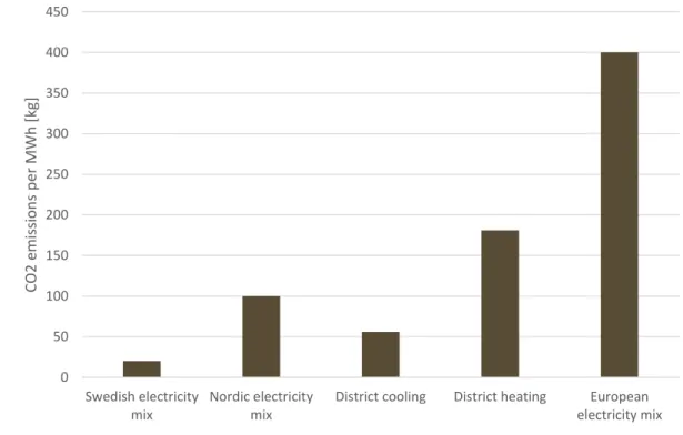
majority of electricity in Sweden is generated by nuclear and hydro power. These power sources account for base load and regulation power in Sweden. Together with other sustainable power sources such as wind power, up to 98 % of the electricity production consists of sources with low emissions of greenhouse gases (Svensk energi (a), 2016). With this mixture, the CO2 emissions are 20 kg/MWh (Svensk Energi (b), 2016).
The electrical grid in Sweden is integrated with the other Nordic countries. Electricity that is used in Sweden is bought on a common Nordic market, Nord Pool, making it more appropriate to use the emissions from the Nordic fuel mixture. Since there is 15 % fossil fuel based electricity production in the Nordic countries combined, the Nordic mixture emits more CO2 than the Swedish mixture. The Nordic mixture emits 100
kg/MWh (Svensk Energi (b), 2016). Further, the grid in Nordic countries is connected to the rest of Europe, where the European mixture is 400 kg/MWh (Svensk Fjärrvärme (a), 2009). In figure 9 CO2 emissions per produced MWh from electricity production
and district heating and cooling production is presented.
Figure 9 Environmental impact in terms of CO2 emission for different energy sources in terms of MWh in kilograms. 0 50 100 150 200 250 300 350 400 450 Swedish electricity mix Nordic electricity mix
District cooling District heating European electricity mix CO2 e m is sion s p er MWh [kg]
16
3.3.3 Emissions from different thermal energy sources
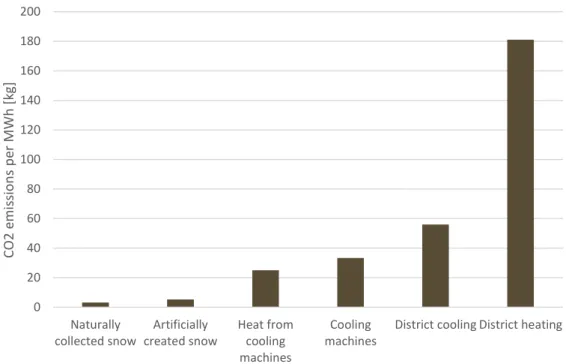
The environmental impact in terms of CO2 emissions for different thermal energy
sources is shown in figure 10. The total emissions will be calculated by taking the energy delivered from different sources, multiplied with the CO2 emission factor.
Figure 10 CO2 emissions per MWh produced thermal energy for evaluated methods in
kilograms.
3.4 Seasonal snow storage
A snow storage could be constructed to cover part of, or the whole, cooling demand for Uppsala University Hospital and Nya Studenternas IP. Since it is possible to create artificial snow with snow canon technologies, the storage does not necessarily need to be dimensioned after the accessibility of natural snow. However, producing artificial snow comes with an expense, both financial and environmental, making it beneficial to maximize the use of the free natural snow while minimizing the use of snow canons. In this model the construction of the storage will be of an open pond design. The location of the storage will remain unspecified. As an insulator, a 0.2 m thick layer of wood chips will be used, reducing natural melt loses to roughly 35 % of the total snow volume. This percentage of losses has been approximated in other studies and is considered an acceptable standard for snow storages with a few meters depth and at least 2 dm of wood chips as insulation (Skogsberg, 2012).
The energy stored within snow is mainly in form of latent energy, which is about 333.7 kJ / kg (92.7 Wh / kg) (Çengel et al, 2007). This energy is stored in the solid phase and is obtained when the snow melts by absorbing heat from the recirculating water.
0 20 40 60 80 100 120 140 160 180 200 Naturally collected snow Artificially created snow Heat from cooling machines Cooling machines
District cooling District heating
CO2 e m is sion s p er MWh [kg]
17
Additional energy is found in the heat of the recirculating water between the intervals 0 to 10 degrees Celsius. The total cooling effect is approximately 100 kWh per ton snow. The total volume of snow stored is dependent on the snow density. Since the densities for snow can vary depending on whether it is naturally or artificially produced a mean value is assumed. Considering that the snow will be compressed when stored, a density of 650 kg per m3 is generalized for this model.
The total amount of snow needed to cover a specific cooling demand can be calculated as follows
𝑉𝑠𝑛𝑜𝑤 = 𝑄𝑑𝑒𝑚𝑎𝑛𝑑
𝑄𝑠𝑛𝑜𝑤∙𝜌𝑠𝑛𝑜𝑤∙(1−𝐿𝐿𝑜𝑠𝑠) [m
3] (1)
Where
- 𝑉𝑠𝑛𝑜𝑤 is the requisite snow volume [m3] - 𝑄𝑑𝑒𝑚𝑎𝑛𝑑 is the total cooling energy demand to be covered [Wh]
- 𝑄𝑠𝑛𝑜𝑤 the cooling energy within snow [Wh kg-1] - 𝜌𝑠𝑛𝑜𝑤the density of snow [kg m-3] - 𝐿𝐿𝑜𝑠𝑠 is the losses in the storage [-]
The corresponding mass of snow is known through
𝑚𝑠𝑛𝑜𝑤 = 𝑉𝑠𝑛𝑜𝑤∙ 𝜌𝑠𝑛𝑜𝑤 [kg] (2)
The total accessible cooling energy stored within the snow storage is calculated as
𝑄𝑎𝑐𝑐𝑒𝑠𝑠 = 𝑚𝑠𝑛𝑜𝑤∙ 𝑄𝑠𝑛𝑜𝑤 [Wh] (3)
Thus the useful cooling energy because of losses is
𝑄𝑢𝑠𝑒𝑓𝑢𝑙 = 𝑄𝑎𝑐𝑐𝑒𝑠𝑠∙ (1 − 𝐿𝐿𝑜𝑠𝑠) [Wh] (4)
By using equation (1), the total useful cooling energy could be calculated by using the available snow from the streets in Uppsala. Uppsala municipality transported 4500 trucks with a volume of 13 m3 from the streets of Uppsala during the winter of 2015 (Bellenox, 2016). This gives a volume of 58 500 m3 of available snow. It is assumed that 50 % of the snow is collected during the last months of the previous year and in January, 40 % in February and 10 % in March. The density of this snow is assumed to be the same as the compressed snow in the storage. Equation 4 gives the total useful cooling energy 2 471.6 MWh.
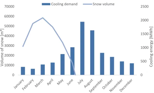
As calculated above, a snow storage would be delivering cooling to the system from April to the beginning of July, as shown in the figure 11.
18
Figure 11 The diagram displays the cooling demand and the volume and remaining energy of the snow storage when the storage is based on the available snow in Uppsala.
According to formula (1) and (2), the total volume and mass of the storage can also be based on the sum of the total cooling demand during the period April - September. The total energy demand during this period is 6 617 MWh. This corresponds to a snow volume of 137 430 m3 with losses.
Figure 12 shows how the cooling capacity stored within the snow storage is utilized and the volume of the snow is decreasing during operation, beginning in April.
Figure 12 The diagram displays total cooling demand and the volume and remaining energy of the snow storage when the storage is based on the total energy demand
during the summer months.
0 500 1000 1500 2000 2500 0 10000 20000 30000 40000 50000 60000 70000 Coo ling en ergy [ MWh ] Volu m e o f sno w [ m ³]
Cooling demand Snow volume
0 500 1000 1500 2000 2500 0 20000 40000 60000 80000 100000 120000 140000 160000 Coo ling en ergy [ MWh ] Volu m e o f sno w [ m ³]
19
When the storage is based on the available natural snow in Uppsala, there is a deficit of energy from the storage. This deficit could be covered up with artificial snow. The artificially created snow has a lower density when produced, but is assumed to be compressed to a density of 650 kg/m3 when stored. The electricity needed to create the snow is approximated to 2 kWh/tonne (Skogberg, 2005). The required artificial snow to be created is 41 454 tonnes. The electricity required to create this amount is 82.9 MWh. Artificial snow combined with natural collected snow can be used to cover the cooling demand for the system. Figure 13 shows how much artificial snow is needed to cover the cooling demand, based on a fixed amount of natural snow.
Figure 13 The amount of natural respectively artificial snow required to cover the cooling demands of Uppsala University Hospital and Nya Studenternas IP during the
period April - September.
In order to estimate an operational energy consumption for the modeled snow storage the cooling capacity is assumed to be an average of the cooling demand. If the cooling energy in the storage were to be delivered evenly over the months of operation, the average delivered cooling capacity would be 1.51 MW.
The cooling capacity is determined by the mass flow and temperature difference of the water during the process, and is calculated as:
𝑃 = 𝑐𝑝∙ 𝑚̇
𝜌 ∙ ∆𝑇 [W] (5)
Where
- cp is the specific heat capacity of water [kJ kg-1K-1]
- ṁ is the mass flow of the water [kg s-1]
2472 4145 6617 Snow Demand Coo ling en ergy [ MWh ]
20
- 𝜌 is the density of water [kg m-3]
According to equation (5) an effect of 1.51 MW corresponds to a water flow of approximately 72 liters per second. Industrial pumps with a total capacity of pumping 72 liters per second operates on a total effect of about 27 kW (Gustafsson, 2016). For the period April to the end of September this would correspond to a total pumping energy of 118.6 MWh.
If the snow storage was to be modeled for the cooling demand of the whole period of April to September artificial snow would have to be created. The total delivery of cooling will then increase as well as the electricity consumption. Table 2 shows cooling delivered and electricity use to deliver that amount of cooling through the snow storage.
Table 2 Cooling capacity with electrical use for the whole period April – September.
Delivered cooling [MWh] Electricity use [MWh]
6 617 201.5
However, if the storage was dimensioned for the amount of natural snow collected in Uppsala, the snow storage would not be able to cover the cooling demand for the period April - September, according to figure (15). The snow canons would in that scenario not be used, resulting in a lower electricity use, but the remaining cooling demand is
covered with district cooling. Table 5 shows the delivered cooling and corresponding electricity use for the scenario without artificially snow created.
Table 1 Cooling delivered with electrical use based on collected amount of natural snow.
Delivered cooling [MWh] Electricity use [MWh]
2 471.6 58
The CO2 emissions will depend on the electricity use during operation. To compact the
snow a piste caterpillar is used. This machine consumes approximately 2000 liters of diesel during operation. One liter of diesel emits approximately 2.7 kg CO2 (EPA,
21
3.5 Cooling Machines
The modeling of the cooling machines will be separated into three sections, winter season, summer season and the two seasons combined.
3.5.1 Winter season
The cooling machines that is used to create and maintain the ice fields at Nya
Studenternas IP are not operational for the most part of the year. They stop running in late March and is not operated again until start of the next season, in mid-October. Moreover, the machines are only operated for ice cooling when the outdoor temperature is above -5 °C when cooling maintenance is required (Lindberg, 2016). Whenever the outside temperature is above -5 °C during the months of ice maintenance, the ice will absorb heat making it a necessity to run the cooling machines. Since the ambient temperature can vary a lot from year to year, the time for which the cooling machines are in operation will also vary. Due to a lack of operating data for the existing cooling machines, simulations in MATLAB were made to get an approximation of the seasonal use of the cooling machines. Monthly averages of outdoor temperatures were calculated based on the years from 2005 to 2015. The difference between the average monthly ambient temperatures and -5 °C was used in equation (6) to get a daily average of the cooling capacity needed.
𝑄𝑖𝑐𝑒 𝑐𝑜𝑜𝑙𝑖𝑛𝑔 = 𝑈𝑖𝑐𝑒∙ 𝐴 ∙ (𝑇𝑎𝑚𝑏𝑖𝑒𝑛𝑡− 𝑇𝑖𝑐𝑒) [W] (6)
Where
- A is the area of the field [m2]
- 𝑈𝑖𝑐𝑒 is the overall heat transfer coefficient from air to ice [W (m-2K-1)]
Due to the second law of thermodynamics the ice will absorb heat from its warmer environment, making a continuous refrigeration of the ice a necessity. The heat transfer coefficient from the air to the ice can be calculated as:
𝑈𝑖𝑐𝑒 = 1 ( 1 ℎ𝑎𝑖𝑟)+( 𝑑 𝐾𝑖𝑐𝑒) [W (m-2K-1)] (7) Where
- d is the thickness of the field [m]
- Kice is the thermal conductivity for ice [W(m-1K-1)]
22
In order to estimate the cooling delivered from the cooling machines, the specific cooling capacity required for each month is calculated in MWh for the months of operation. The delivered cooling during the winter season can be seen in figure 14.
Figure 14 The corresponding energy required to be delivered each month by the cooling machines in order to keep the ice at a temperature of -5 degrees.
The cooling machines at Nya Studenternas IP are assumed to have a nominal cooling capacity of 2 800 kW and a COPcooling of 3 (Lindberg, 2016). An approximation of the
electrical input to operate the compressor can be calculated by using equation (8):
𝐶𝑂𝑃𝑐𝑜𝑜𝑙𝑖𝑛𝑔 = 𝑄𝑐𝑜𝑙𝑑̇
𝑃𝑐𝑜𝑚𝑝 [-] (8)
Where
- 𝑄𝑐𝑜𝑙𝑑 is the cooling effect produced [W] - Pcomp is the input work as electricity [W]
According to formula (9) the heat effect delivered is the sum of electrical input to operate the compressor and the heat absorbed from the ice.
𝑄̇ℎ𝑒𝑎𝑡 = 𝑄̇𝑐𝑜𝑙𝑑+ 𝑃𝑐𝑜𝑚𝑝 [W] (9)
The given and calculated specifications and properties of the cooling machines can be seen in table 3.
23
Table 3 Specifications and properties of the cooling machines.
Cooling capacity 2 800 kW
Heating capacity 3 733 kW
COPcooling 3
COPheating 4
Electrical input 933 kW
During operation, the cooling machines will move heat from the ice that can be obtained and used. The total amount of heat removed each month is described in formula (10). It is assumed that the machine only provides cooling to the ice during this period of time. In figure 15 the delivered cooling and heating, and the electricity input are presented.
𝑄ℎ𝑒𝑎𝑡 = (𝑄̇𝑐𝑜𝑙𝑑+ 𝑃𝑐𝑜𝑚𝑝) ∙ 𝑡 [Wh] (10)
Where
- t is the amount of operating hours per month [h]
Figure 15 The required electricity input needed to cool the ice per month and the amount of heat that can potentially be obtained from the cooling machines during the
season. Observe that the cooling machines are only operational for the latter half of October and the first half of March.
24
3.5.2 Summer season
During the warmer periods of the year, ranging from April to September the cooling machines are not operational. However, if the cooling machines were to be used to support cooling to Nya Studenternas and Uppsala University Hospital, the total need for district cooling could be reduced. In the process of cooling these facilities, heat would be obtained which could then be utilized. The cooling machines offers a total cooling capacity of 2 800 kW continuously. This cooling effect corresponds to approximately 2016 MWh per month if the cooling machines were to be operated constantly. Figure 16 below shows the monthly amount of heat that is obtained when the cooling demand of Uppsala University Hospital and Nya Studenternas IP is covered with the cooling machines.
Figure 16 The amount of heat obtained and input work when producing cooling matching the demands of Uppsala University Hospital combined with Nya Studenternas
during the summer season.
3.5.3 Total annual production
In this model the cooling machines are operated for most part of the year, absorbing heat from different areas depending on the season. Heat is obtained from the cooling machines during the whole year, which could be utilized and used in order to reduce district heating and cooling demands. In figure 17 the total annual delivery from the machines are presented. How the absorbed heat could be utilized is described closer in the next section (section 3.6).
25
Figure 17 Total annual delivery of cooling and heating to the facilities from the cooling machines with corresponding electrical power consumption to the system, in MWh.
3.6 Hot water storage
For both Uppsala University Hospital and Nya Studenternas IP, district heating covers their demand for comfort heating and hot water. For Uppsala University Hospital the hot water is about 27 % of their district heating demand displayed in figure 5 (Nystrand, 2016). Therefore, the hot water demand of the hospital has been modeled as 27% of its annual district heating demand evenly distributed over the moths. Nya Studenternas IP’s hot water demand is based on a prediction, which states that the sports arena will
consume 105 096 kWh of hot water per year (Quarfordt, 2016). In order to distribute the hot water demand of the sports arena over a year, it was fitted with the monthly
distribution made in a similar study conducted by Belgian Building Research Institute (Gerin, Bleys and De Cuyper, 2014, p 4). The resulting hot water demands are found in table 4.
26
Table 4 Estimated monthly hot water demand for Uppsala University Hospital and Nya Studenternas IP.
Uppsala University Hospital Nya Studenternas IP Total
Jan 1 482 991 9 546 1 492 537 Feb 1 482 991 9 984 1 492 975 Mar 1 482 991 9 459 1 492 449 Apr 1 482 991 9 021 1 492 011 May 1 482 991 8 670 1 491 661 Jun 1 482 991 8 233 1 491 223 Jul 1 482 991 7 094 1 490 085 Aug 1 482 991 7 269 1 490 260 Sep 1 482 991 8 233 1 491 223 Oct 1 482 991 8 846 1 491 836 Nov 1 482 991 9 196 1 492 187 Dec 1 482 991 9 546 1 492 537
The potential sources of thermal energy for water heating are:
● Thermal energy generated by the solar collectors placed on the F-house roof ● Excess heat from Nya Studenternas IP’s cooling machines
Below follows the formulas used in order to calculate thermal energy supply from solar collectors, equation (11), and predict the capacity of a potential hot water storage, equation (12).
27 Thermal energy obtained from solar collectors:
𝑄𝑠𝑜𝑙𝑎𝑟 ≈ 𝜂𝑜𝑝𝑡.⋅ 𝜂𝑡ℎ𝑒𝑟𝑚.⋅ 𝐼𝑠𝑜𝑙𝑎𝑟⋅ 𝐴𝑠𝑜𝑙𝑎𝑟 [kWh] (11)
Where:
𝑄𝑠𝑜𝑙𝑎𝑟 - Thermal energy from solar collectors [kWh]
𝜂𝑜𝑝𝑡. - Optical efficiency [-]
𝜂𝑡ℎ𝑒𝑟𝑚. - Thermal efficiency [-]
𝐼𝑠𝑜𝑙𝑎𝑟 - Solar irradiance [kWh/m2]
𝐴𝑠𝑜𝑙𝑎𝑟 - Area covered by solar collectors [m2]
As for the amount of stored thermal energy, it varies depending on whether the supply is greater than the demand or the other way around. Hence equation (12) has been divided into three parts. The first part (1), is used for months where the thermal energy yield is greater than the demand and therefore offers a possibility to store heat. Part (2) applies for months where there is a thermal energy deficit but the heat storage is not yet emptied. The third and last part, part (3), represents the months with energy deficit where the storage has already been emptied.
Stored amount of thermal energy at a given month (set of equations):
(1) 𝑆𝑡𝑀= 𝑠𝑡𝑐⋅(𝑆𝑡𝑀−1+ 𝐸𝑀)
(2) 𝑆𝑡𝑀 =(𝑠𝑡𝑐⋅ 𝑆𝑡𝑀−1)− 𝐸̂𝑀 (3) 𝑆𝑡𝑀= 0
} (12)
Where:
𝑆𝑡𝑀 - Stored thermal energy at month M [Wh] 𝑠𝑡𝑐 - Heat storage coefficient [-] 𝑆𝑡𝑀−1 - Energy stored during previous month [Wh]
𝐸𝑀 - Surplus energy generated month M [Wh]
28
Solar collectors are to be installed on an area of 125 m2 on the roof of Nya Studenternas
IP’s office building, the F-house. The solar collectors that are going to be installed are the model Vitosol 200-F, which has an optical efficiency of 79.3 % (Viessman, Vitosol 200-F, p 4). Their thermal efficiency varies over the year and the variation is displayed in table 8. To avoid detailed and complex variables, such as relation between circulating fluid temperature in solar collectors and ambient temperature, the thermal efficiency varies in accordance with a study conducted on seasonal thermal efficiency of solar collectors. (Gorjian, Hashjin, Ghobadian and Banakar, 2015, p 501) The solar irradiance is based on data for Stockholm and can be found in table 5 (Fältström and Nilsson, 2012, p 20). Based on this, the amount of thermal energy output from the solar
collectors for each month has been calculated using equation 11. The resulting thermal energy output is shown in figure 18. In addition to this the thermal energy output from the solar collectors is illustrated in proportion to the hot water demand of Nya
Studenternas IP in figure 19.
Table 5 Variation of solar irradiance [kWh/m2] and thermal efficiency experienced by the solar thermal collectors on the F-house roof.
Jan Feb Mar Apr May Jun Jul Aug Sep Oct Nov Dec
𝐼𝑠𝑜𝑙𝑎𝑟 10 26 68 110 164 174 165 130 78 36 12 6
𝜂𝑡ℎ𝑒𝑟𝑚. 0.66 0.69 0.70 0.73 0.74 0.77 0.78 0.77 0.76 0.74 0.70 0.64
29
Figure 19 Illustration of proportion between yielded energy from solar collectors and Nya Studenternas hot water demand
By adding the thermal energy yielded from the solar collectors (figure 18) with the excess heat generated by the cooling machines (figure 16 and 17) the total monthly supply of energy for hot water is obtained. The obtained energy available for hot water suggests that the cooling machines run the entire summer, unlike the case of the
integrated energy system solution for cooling. Table 6 shows the total energy supply, what percentage of the total hot water demand it covers, and the monthly deviation between supply and demand. The deviation, together with the set of equations referred to as equation 12, has been used to calculate the possibilities of storing the hot water.
30
Table 6 Thermal energy supplied by solar collectors and cooling machines, its coverage of the total hot water energy demand and the difference between demand and supply.
Thermal energy supplied by solar collectors and cooling
machines [MWh]
Coverage of total hot water demand [%] Difference between supply and demand [MWh] Jan 326 21.8 -1 167 Feb 680 45.5 -813 Mar 460 30.8 -1 032 Apr 614 41.2 -878 May 1 030 69.1 -462 Jun 1 367 91.7 -124 Jul 2 604 175 1 114 Aug 2 185 147 695 Sep 1 084 72.7 -407 Oct 1 401 93.9 -91 Nov 1 641 110 149 Dec 1 175 78.7 -318
A heat storage coefficient, much similar to a monthly efficiency of the hot water
storage, has been used in order to estimate the possibility to store excess thermal energy over seasons. The coefficient is set to 0.79 (21 % thermal losses per month) which is the lowest value that can generate a storage which lasts throughout December. A sensitivity analysis of this coefficient will be presented later on in section 5.2. Figure 20 illustrates the amount of energy stored in the hot water storage after the monthly demand has been satisfied. The thermal energy storage has been calculated using the set of equations referred to as equation 12.
31
Figure 20 Amount of thermal energy present in the hot water storage at given months. Heat storage coefficient is set to 0.79.
0 0 0 0 0 0 880 1244 576 364 405 2,42
Jan Feb Mar Apr May Jun Jul Aug Sep Oct Nov Dec
Sto re d t h erm al en ergy [MWh ]
32
4. Results
The results of the modeled solutions for energy alternatives will be presented below. There will be a comparison of the presently used energy sources were CO2 emission reduction will be in focus. When the emissions from the energy solutions are presented, a Nordic electrical mixture is used.
4.1 Snow storage
The snow storage would be a new solution that could deliver cooling to the facilities. By having a storage with a volume of 137 430 m3, the total cooling demand during the
summer could be covered. However, the available snow in Uppsala varies from year to year. By assuming that the average volume of available snow is 58 500 m3, there is a deficit of 40 391 tonnes snow that has to be produced with snow canons. To create this amount of snow 82.9 MWh electricity is needed. In order to maintain a water flow in the circulating system, 118.6 MWh of electricity is required.
The scenario where the deficit volume of snow is chosen not to be artificially produced, the cooling capacity delivered by the snow storage is limited to what is naturally
collected in the local areas. With a snow collection of 58 500 m3 and cooling capacity of 2 471.6 MWh, the storage would last until the start of July. Supporting the system with this amount of cooling would require an electricity input to operate the pumps of 58 MWh. The rest of the cooling energy required for July, August and September would in this scenario be supplied with district cooling.
Figure 21 CO2 emissions in tonnes for the summer period of April - September for
district cooling use versus a combination of snow storage and district cooling.
0 50 100 150 200 250 300 350 400
District cooling District cooling and snow storage Snow storage CO2 e m is sion s [to n n es ] April - september
33
The reduction of CO2 emissions provided by the solutions can be seen in figure 21 and
is about 345 tonnes for the snow storage used the whole summer season. This amount corresponds to a decrease of 93.1 % compared to sole use of district cooling the given period. The emissions from a snow storage complemented with district cooling is 127.2 tonnes. This amount corresponds to a decrease of 34.3 % compared to sole use of district cooling the given period.
4.2 Cooling machines
The cooling machines at Nya Studenternas IP can be considered an untapped resource. If the cooling machines were to be utilized for the whole year, cooling and heat would be obtained in exchange for electrical input.
During the summer season, ranging from April to end of September, the cooling machines could supply the system with both cooling and heating energy.
The cooling machines have the capacity to deliver cooling to the system that would completely eliminate the need for district cooling during the summer season. In addition, the cooling machines produces heat that covers a portion of the heating demands for the same season. Seen in figure 22.
Figure 22 Reduction of district heating through cooling machines over the summer. The excess heat generated (negative in the diagram) during July and August is stored and
used in September. -1500 -500 500 1500 2500 3500 4500 5500 6500
April May June July August September
H eat in g D em an d [MWh]
34
Figure 23 CO2 emissions in tonnes of sole use of district heating and cooling (left), and
the emissions with contribution of cooling machines (right) during the summer season. The emissions from district cooling this period is eliminated.
According to figure 23, the contribution of cooling machines to the system reduces the amount of CO2 emissions released to the atmosphere by 1 747 tonnes during the
summer. This amount corresponds to a CO2 emission reduction of 49 % during this
period.
During the winter season ranging from mid of October to mid of March the cooling machines will only deliver cooling to the ice fields. The obtained heat that could in theory be utilized to reduce district heating is displayed in figure 24.
35
Figure 24 The reduced need for district heating when the cooling machines are delivering heat for the winter season.
Adding together the uses of the cooling machines for both seasons gives a total annual district heating and cooling use reduction seen in figure 25. In figure 26, the annual reduction of CO2 emissions is shown for the use of cooling machines.
Figure 25 The total demand of heating and cooling is split up between district heating, district cooling and the use for the cooling machines for a year.
0 2000 4000 6000 8000 10000 12000
October November December January February Mars
He at dem an d [MW h] District heating 0 10000 20000 30000 40000 50000 60000 70000 80000
Heating demand Cooling demand
En er gy [M Wh ] District heating
Heat from cooling machines District cooling
Cooling from cooling machines
36
Figure 26 CO2 emissions in tonnes of sole use of district heating and cooling (left), and
the emissions with contribution of cooling machines (right).
According to the diagram above the contribution of cooling machines to the system reduces the amount of CO2 emissions released to the atmosphere by 2 484 tonnes. This
amount corresponds to an annual CO2 emission reduction of 20.6 %.
4.3 Snow storage and cooling machine integration
A combination of cooling systems could be integrated and used to deliver cooling by using a snow storage based on the naturally available snow in Uppsala and the cooling machines to cover the rest of the cooling demand. Heat will also be delivered from the cooling machines. During the first three months, when the snow storage is operational, heat is obtained through district heating while the three last months is mainly covered with the heat from cooling machines. This scenario will result in reducing both district cooling and heating demand. In figure 27 the left diagram displays how the monthly cooling demands can be covered using naturally collected snow in a snow storage the first three months of the summer and then the last three months is covered with cooling machines. The right diagram shows how the heating demands can be covered with a combination of heat from the cooling machines and district heating. The CO2 emissions
released to the atmosphere using this thermal energy system is presented in figure 28.
0 2000 4000 6000 8000 10000 12000 14000
District heating and cooling usage Support of cooling machines
CO2 e m m is ion s [to n n es ]
37
Figure 27 Thermal energy from integrated energy solutions during the summer season.
Figure 28 CO2 emissions in tonnes of sole use of district heating and cooling (left), and
the emissions with contribution of snow storage until July and cooling machines until September (right). The emissions from district cooling this period is eliminated.
The reduction of CO2 emissions provided by this solution is presented in figure 28 and
is about 1 276 tonnes. This amount corresponds to a decrease of 36 % compared to the CO2 emissions of sole use of district heating and cooling the given period.
4.4 Hot water storage
The estimated seasonal demands of thermal energy in terms of hot water use for Uppsala University Hospital and Nya Studenternas IP are a part of the demand for district heating. They can be found in table 4 in the modeling chapter.
38
Provided that the hot water storage uses only the solar collectors and cooling machines as heating sources and that it can maintain the amount of thermal energy in accordance with the heat storage factor 0.79, it will be able to replace the district heating as
presented in table 7.
Table 72 Coverage status of hot water storage supplied with heat by solar collectors and cooling machines.
Surplus energy or energy deficit Coverage status
January Deficit Insufficient coverage, storage empty
February Deficit Insufficient coverage, storage empty
March Deficit Insufficient coverage, storage empty
April Deficit Insufficient coverage, storage empty
May Deficit Insufficient coverage, storage empty
June Deficit Insufficient coverage, storage empty
July Surplus Sufficient coverage, surplus energy stored
August Surplus Sufficient coverage, surplus energy stored
September Deficit Sufficient coverage using stored energy
October Deficit Sufficient coverage using stored energy
November Surplus Sufficient coverage, surplus energy stored
December Deficit Sufficient coverage using stored energy
The energy stored during July, August and November could in this case provide both Uppsala University Hospital and Nya Studenternas IP with hot water during September, October and December. Some complementary source of thermal energy, district heating for instance, would still be needed in order to cover the hot water demand January-June. Since the cooling machines and solar collectors are still productive, though not enough to cover the entire demand, during these months, the use of district heating would still be reduced if these solutions were implemented. In accordance with table 7, the estimated annual reduction of district heating is displayed in figure 29.
39
Figure 29 Estimated reduction of district heating for hot water demand if using the solar collectors and cooling machines as heat sources for a hot water storage.
In total, a hot water storage with a heat storage coefficient of 0.79 would, together with the heat generated by cooling machines and solar collectors, be able to cover 75.0 % of the annual hot water demand.
For environmental impacts of the hot water storage, see the environmental impacts of the cooling machines, section 4.2.
4.5 Results summary
Summary of results when using a Nordic electrical mixture will follow in table 8.
Table 8 Reduction of CO2 emissions during the summer season compared to full use of
district heating and cooling.
Solution Reference Reduction [%]
Snow storage District cooling 93.1 District cooling and snow
storage
District cooling 34.3
Cooling machines District cooling and heating
49
Snow storage and cooling machines
District cooling and heating 36 0 200 400 600 800 1000 1200 1400 1600 1800
Jan Feb Mar Apr May Jun Jul Aug Sep Oct Nov Dec
Th erm al en ergy [ MWh ] District heating Hot water solutions
40
5. Sensitivity Analysis
A sensitivity analysis has been made to evaluate how the environmental impacts for the modeled solutions depends on the emittance of CO2 per produced MWh electricity. For
the heat storage the coefficient for heat loss in storage is analyzed. This to evaluate the result.
5.1 CO
2emissions for different electricity mixtures
Depending on what type of electricity mixture is used to operate the pumps, cooling machines and, snow canons, which were presented in the modeling section, the
environmental impact will vary. A sensitivity analysis of the total CO2 emissions during
the summer season has been made for four modeled solutions. These present how sensitive each solution is for changes of electricity production. The x-axis displays how the CO2 emissions from electricity production vary and the corresponding total CO2
emissions for the different solutions on the y-axis. The analysis starts with a Swedish mixture of 20 kg/MWh and is then increased, and the emissions from district cooling and heating will be constant.
Figure 30 presents the total amount of CO2 emissions for different cooling solutions
with sole use of district cooling as reference.
Figure 30 Sensitivity analysis for cooling supplement during the summer season for the different modeled solutions. Each line represents the CO2 emissions produced when
41
Sole supplement by cooling machines and a combination of snow storage and cooling machines are the two most sensitive solutions to variations of CO2 emissions per MWh
produced electricity. When the electricity production emits more than approximately 170 kg/MWh respectively 250 kg/MWh, these solutions are emitting more CO2 than by
using district cooling. The solutions based on snow storage are however less sensitive and are emitting less CO2 than sole use of district cooling this given interval.
Corresponding diagram for heating is displayed in figure 31 with sole use of district heating as reference.
Figure 31 Sensitivity analysis for heating supplement during the summer season for the presented modeled solutions. The diagram represents the CO2 emissions produced when
covering the seasonal heating demands with variated emissions per MWh produced electricity.
Using the heat generated from the cooling machines in combination with district heating for the energy shortage emits less than a sole use of district heating, or a use of the combination with a snow storage, until the CO2 emissions is above 730 kg per produced
MWh electricity. This solution is however more sensitive than the combination with a snow storage, where the latter will emit less when the CO2 emissions is above 730 kg
per produced MWh electricity.
In figure 32, the CO2 emissions for both heating and cooling is displayed. Reference is
the sum of emissions from heating and cooling using solely district heating and district cooling.
42
Figure 32 Sensitivity analysis for both heating and cooling for the summer season with the total thermal energy demands as reference. Each line represents a modeled solution
covering both the heating and cooling demands with the total CO2 emissions on the
y-axis. Cooling supplement / Heating supplement is used as notation.
The use of snow storage as cooling source with heating supplement of district heating is the most robust solution presented. However, using snow storage in combination with cooling machines as cooling source while supplying heat through district heating and from cooling machines, results in a more sensitive solution but has the potential to emit less CO2 emissions. The solution with sole use of cooling machines as cooling
supplement and heat demand is covered with district heating and heat from cooling machines, emits the least of the solutions until the CO2 emissions per produced MWh electricity is above 190 kg/MWh. When the emissions from electricity is more than 190 kg/MWh, the combination with a snow storage is the least emitting solution.
5.2 Hot water storage
Here follows a sensitivity analysis regarding the heat storage coefficient for the hot water storage. The value used in the modeling of the hot water storage, 0.79, has been compared to one of 0.63, which is the limit in order for the stored heat to last throughout October, and to one of 1.0, which is an ideal but unrealistic case. The results can be seen in figure 33.
43
Figure 33 Stored thermal energy (left) and the resulting coverage of the total hot water demand (right). The heat storage coefficient varies and is 0.79 for section A, 0.63 for
section B, and ideal (1.0) for section C.
As can be seen in figure 33 not even an ideal hot water storage is enough to cover the annual hot water consumption. The gap between supply and demand is too great. A heat storage coefficient between 0.63 and 0.79 is enough for the storage to last 2-3 months of deficit. The heat storage coefficient of 0.79 is equal to 75.0 % coverage on an annual basis. Corresponding coverage for the other coefficients are 73.6 % (B) and 81.4 % (C).