The HARPS search for southern extra solar planets XLIII A compact system of four super Earth planets orbiting HD 215152

February 14, 2018

The HARPS search for southern extra-solar planets

XLIII. A compact system of four super-Earth planets orbiting HD 215152

J.-B. Delisle

_{, D. Ségransan}

_{, X. Dumusque}

_{, R.F. Diaz}

_{, F. Bouchy}

_{, C. Lovis}

_{, F. Pepe}

_{, S. Udry}

_{, R. Alonso}

_,

W. Benz

_{, A. Co}

_ffi

_net

_{, A. Collier Cameron}

_{, M. Deleuil}

_{, P. Figueira}

_{, M. Gillon}

_{, G. Lo Curto}

_{, M. Mayor}

_,

C. Mordasini

_{, F. Motalebi}

_{, C. Moutou}

_{, D. Pollacco}

_{, E. Pompei}

_{, D. Queloz}

_{, N.C. Santos}

_{, and}

A. Wyttenbach

1 _{Observatoire de l’Université de Genève, 51 chemin des Maillettes, 1290, Sauverny, Switzerland}

e-mail:[email protected]

2 _{ASD, IMCCE, Observatoire de Paris - PSL Research University, UPMC Univ. Paris 6, CNRS,}

77 Avenue Denfert-Rochereau, 75014 Paris, France

3 _{Universidad de Buenos Aires, Facultad de Ciencias Exactas y Naturales, Buenos Aires, Argentina}

4 _{CONICET - Universidad de Buenos Aires, Instituto de Astronomía y Física del Espacio (IAFE), Buenos Aires, Argentina}

5 _{Instituto de Astrofísica de Canarias, 38205 La Laguna, Tenerife, Spain,}

6 _{Dpto. de Astrofísica, Universidad de La Laguna, 38206 La Laguna, Tenerife, Spain}

7 _{Physikalisches Institut, Universitat Bern, Silderstrasse 5, CH-3012 Bern, Switzerland}

8 _{School of Physics and Astronomy, University of St Andrews, North Haugh, St Andrews, Fife KY16 9SS}

9 _{Aix Marseille Université, CNRS, LAM (Laboratoire d’Astrophysique de Marseille) UMR 7326, 13388, Marseille, France}

10 _{Instituto de Astrofísica e Ciências do Espaço, Universidade do Porto, CAUP, Rua das Estrelas, 4150-762 Porto, Portugal}

11 _{Institut d’Astrophysique et de Géophysique, Université de Liège, Allée du 6 Août 17, Bat. B5C, 4000, Liège, Belgium}

12 _{European Southern Observatory, Karl-Schwarzschild-Str. 2, D-85748 Garching bei München, Germany}

13 _{Canada France Hawaii Telescope Corporation, Kamuela, 96743, USA}

14 _{Department of Physics, University of Warwick, Coventry, CV4 7AL, UK}

15 _{Cavendish Laboratory, J J Thomson Avenue, Cambridge, CB3 0HE, UK}

16 _{Departamento de Física e Astronomia, Faculdade de Ciências, Universidade do Porto, Rua do Campo Alegre, 4169-007 Porto,}

Portugal February 14, 2018

ABSTRACT

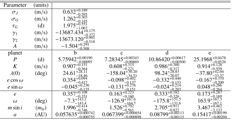
We report the discovery of four super-Earth planets around HD 215152, with orbital periods of 5.76, 7.28, 10.86, and 25.2 d, and

minimum masses of 1.8, 1.7, 2.8, and 2.9M⊕respectively. This discovery is based on 373 high-quality radial velocity measurements

taken by HARPS over 13 years. Given the low masses of the planets, the signal-to-noise ratio is not sufficient to constrain the planet eccentricities. However, a preliminary dynamical analysis suggests that eccentricities should be typically lower than about 0.03 for the system to remain stable. With two pairs of planets with a period ratio lower than 1.5, with short orbital periods, low masses, and low

eccentricities, HD 215152 is similar to the very compact multi-planet systems found byKepler, which is very rare in radial-velocity

surveys. This discovery proves that these systems can be reached with the radial-velocity technique, but characterizing them requires a huge amount of observations.

Key words. planetary systems – planets and satellites: general – planets and satellites: detection – planets and satellites: dynamical

evolution and stability

1. Introduction

The properties of extrasolar planetary systems are very diverse and often very different from those in the solar system (e.g.,

Mayor et al. 2014). Transit surveys, and especially the Kepler

telescope, have discovered many systems of super-Earth plan-ets in compact orbital configurations. In particular,Keplerfound many systems with period ratios (Pout/Pin) lower than 1.5 (

Lis-sauer et al. 2011; Fabrycky et al. 2014). These compact

plan-etary systems raise several interesting questions regarding their formation and long-term evolution, such as whether these

sys-? _{The HARPS data used in this article are available in electronic form}

at the CDS via anonymous ftp to cdsarc.u-strasbg.fr (130.79.128.5) or

viahttp://cdsweb.u-strasbg.fr/cgi-bin/qcat?J/A+A/.

tems formed in situ or by converging migration of the planets in the proto-planetary disk, and the role played by mean-motion resonances in setting up their architecture and in their long-term stability. These questions are still open, and new observa-tional data would help in better constraining the formation mod-els. While compact systems are favored by observational biases in transit surveys (e.g.,Steffen & Hwang 2015), such systems

are particularly challenging to separate with the radial velocity (RV) method. To our knowledge, only three pairs of planets with

Pout/Pin<1.5 have been found using the RV technique: – HD 5319b and c, giant planets with Pout/Pin = 1.38 (see

Robinson et al. 2007;Giguere et al. 2015),

– HD 200964b and c, giant planets withPout/Pin =1.34 (see

Johnson et al. 2011), and

Table 1.Stellar properties of HD 215152.

Parameter (units)

M (M) 0.77±0.015

R (R) 0.73±0.018

Spectral type K3V1

Prot (d) 42 logR0

HK -4.86

vsini (km/s) 3.352

Teff (K) 4935±763

[Fe/H] −0.10±0.043

MV (mag) 6.453

B−V (mag) 0.994

π (mas) 46.24±0.265

logg (cgs) 4.403

Notes.(1)_{Gray et al.(2003) ,}(2)_{Martínez-Arnáiz et al.(2010) .}(3)_Sousa et al.(2008) ,(4)_{Høg et al.(2000) ,}(5)_{Gaia Collaboration et al.(2016)}

– GJ 180b and c, super-Earth planets withPout/Pin=1.40 (see

Tuomi et al. 2014).

Only one of these systems consists of super-Earth planets (GJ 180). Several other systems have been claimed, but were subsequently contested (e.g.,Díaz et al. 2016).

In this article we present a system of four super-Earth plan-ets around HD 215152, with periods of 5.76, 7.28, 10.86, and 25.2 d (period ratios of 1.26, 1.49, and 2.32). Such a compact system of super-Earth planets is very similar to the compact sys-tems found byKepler. Separating these signals required a huge observational effort, in which 373 high-quality HARPS RV

mea-surements were taken over 13 years.

In Sect.2we describe the stellar properties and the data we used. We then describe the method we employed to analyze the data in Sect.3. In Sect.4we assess the orbital stability of the sys-tem and deduce additional constraints on the orbital parameters. Finally, we discuss our results in Sect.5.

2. HARPS data and stellar properties

We present here 373 RV measurements of the K-dwarf HD 215152 that have been obtained with the HARPS high-resolution spectrograph mounted on the 3.6m ESO telescope at La Silla Observatory (Mayor et al. 2003). The observations span 13 years, from June 2003 to September 2016. The optical fibers feeding the HARPS spectrograph were changed in May 2015

(Lo Curto et al. 2015), which results in an offset between the

284 measurements taken before and the 89 measurements taken after the upgrade. The RV points have been taken in 330 diff

er-ent nights. Of these 330 nights, 287 have a single point, and 43 have two points.

Dumusque et al. (2015) found that the stitching of the

HARPS detector could introduce a spurious RV signal of small amplitude with periods close to one year or an harmonic of it. The stitching of the detector creates pixels of different sizes

ev-ery 512 pixels in the spectral direction, which perturbs the wave-length solution that is obtained by interpolating the wavewave-length of the thorium emission lines on an even scale. Owing to the barycentric Earth RV, the spectrum of a star is shifted on the CCD in the spectral direction, and some lines can cross stitches. When this is the case, the mismatch in the wavelength solution at the position of the stitch creates a spurious RV effect, which,

−10 −5 0 5

∆

v

(m

/

s)

−2000 −1000 0 1000 2000

t(BJD−2455000.0)

−5.00 −4.95 −4.90 −4.85 −4.80

log

R

0 HK

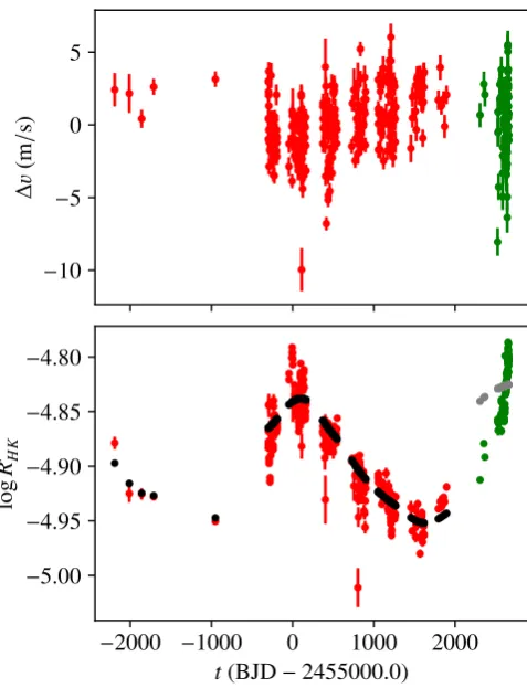
Fig. 1.Time series of the RV (top) and the logR0

HKactivity index

(bot-tom).Red(green) dots correspond to HARPS data taken before (after)

the fiber upgrade. The smoothed activity index, described in Sect.3.1,

is superimposed (blackandgraydots) over the raw logR0

HKvalues for

comparison. We observe a long-term evolution in the RVs that is

anti-correlated with the magnetic cycle (long-term evolution of the logR0

HK).

coupled with the shift of the spectrum on the CCD over time, creates a signal typically with the period of the rotation of Earth around the Sun or an harmonic of it. To remove this spurious sig-nal from the data, we adopted the method proposed inDumusque

et al.(2015), that is, we removed all the lines that crossed stitches

from the computation of the RV .

In addition to the RVs, we also derived the logR0

HK activity index from each of the 373 spectra. As for the RV, this index might also be affected by the fiber upgrade. The RV and logR0_HK

measurements are shown in Fig.1. We also provide a brief sum-mary of the properties of HD 215152 in Table1. The mass and the radius of the star as well as their uncertainties were de-rived using the Geneva stellar evolution models (Mowlavi et al. 2012). The interpolation in the model grid was made through a Bayesian formalism using observational Gaussian priors onTeff,

MV, logg, and [Fe/H] (Marmier 2014). The rotation period of the star, estimated usingMamajek & Hillenbrand(2008) andNoyes

et al.(1984), is 42 days. HD 215152 is a quiet star similar to

the Sun, with a mean logR0

HK of−4.86 and values between−5 and−4.8 (see Table1and Fig.1). However, we clearly observe

a long-term evolution in the logR0

HK activity index, with a pe-riod of about 3,000 d (see Fig.1). This evolution is most likely related to the magnetic cycle of the star. We also observe a long-period signal in the RVs, which is anticorrelated with the signal found in the activity index (see Fig.1). Using only the data taken before the fiber upgrade (to avoid offset issues), we find a

100 ₁₀1 ₁₀2 ₁₀3 ₁₀4

P(d)

0.0 0.2 0.4 0.6 0.8 1.0

Normalized

po

wer

raw activity smoothed activity residuals

Fig. 2.Periodogram of the raw activity (logR0

HK index, inred), the

smoothed activity (see Sect.3.1, ingreen), and the residuals of the

activ-ity after the smooth component is subtracted (ingray). The smoothed

activity captures the long-term evolution of the logR0

HK index and

re-duces the high-frequency part of the signal.

et al. 2016) between the RVs and the logR0

HK index. This anti-correlation is surprising since a anti-correlation is usually found (and expected) on the timescale of the magnetic cycle (Lovis et al.

2011;Dumusque et al. 2011). However, for late-K and M stars,

the correlation might reverse (Lovis et al. 2011, Fig. 18), which might be evidence for convective redshift (Kürster et al. 2003).

3. Analysis

We modeled the RVs of HD 215152 as follows: For thek-th data point, we have

v(tk)=vKep(tk)+γi+Mag.cycle(tk)+k, (1) wherevKep(tk) is the Keplerian motion of the star,γi is the ra-dial proper motion of the system plus instrumental offset (one

independent constant for each instrument), Mag.cycle(tk) is the component of the RV generated by the magnetic cycle of the star, andkis the noise. We here only worked with a single instrument (HARPS), but since the fiber upgrade of May 2015 might induce an offset, we considered measurements before and after the fiber

upgrade as coming from two independent instruments, and intro-duced two constantsγ1(before) andγ2(after). The noise termk in Eq. (1) takes the white and the correlated components of the noise into account (instrumental error, short-term activity of the star, etc.).

3.1. Magnetic cycle correction

In order to account for the effect of the magnetic cycle on the

RVs (see Sect.2), we introduce a proportionality coefficient

be-tween the RVs and the activity index in our model. While an (anti)correlation is expected between the two quantities on long timescales because of the magnetic cycles, on shorter timescales, other effects might break this correlation (stellar rotation,

ap-pearing and disapap-pearing active regions, or different types of

ac-tive regions). In order to avoid introducing artificial short-term signals in the RVs, we first filtered the logR0

HK index to keep only the long-term trend by averaging it using a Gaussian kernel.

100 ₁₀1 ₁₀2 ₁₀3 ₁₀4

P(d)

−5 0 5 10 15 20

log

BF

model w/o mag. cyc.

model w/mag. cyc.

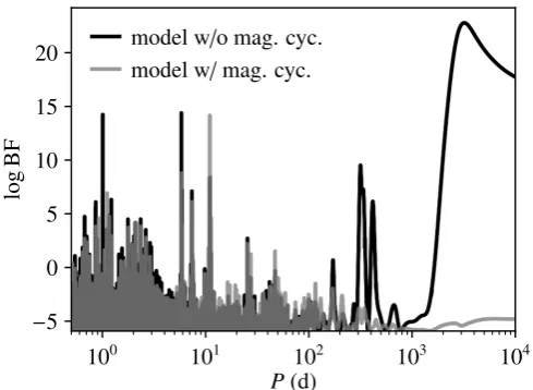
Fig. 3.Periodogram of the RVs using two different models. The first (black) does not include the corrections for magnetic cycles, while the

second (gray) does includes them (see Sect.3.1). The main peak in the

blackcurve is around 3,000 d (similar to the period observed in the logR0

HK). This peak disappears when the magnetic cycle is corrected

for (graycurve).

We used a six-month width for the Gaussian kernel, which ap-proximately corresponds to one observational season, in order to clean the high-frequency part of the logR0

HKwhile preserving the 3,000 d cycle. Since there might be a small offset in the logR0_HK

values after the fiber change, we filtered the two data sets inde-pendently. The smoothed activity index is shown in Fig.1, super-imposed with the initial logR0

HKindex. In Fig.2we also compare the periodogram of the raw logR0

HK index, the smoothed activ-ity index, and the residuals of the logR0

HK after subtracting this smooth component. For these periodograms, we adjusted for a possible offset between the data taken before and after the fiber

upgrade. We observe, as expected, that the smoothed activity in-dex captures the long-term evolution of the logR0

HK index while cleaning the high-frequency part of the signal (see Fig.2). We do not observe any significant signal at the rotation period of the star (around 42 d) in the periodogram of the residuals of the logR0

HKindex (see Fig.2).

The magnetic cycle component in Eq. (1) is thus given in this simple model by

Mag.cycle(tk)=A×smoothed activity_k, (2)

whereAis the proportionality coefficient that is to be adjusted.

In order to have velocity units for Aand to minimize correla-tions betweenAandγi, we rescaled and centered the smoothed activity indicator to have a zero mean and a semi-amplitude of one.

The magnetic cycle component of Eq. (2) might introduce an offset in our model before and after the fiber change as a result of

the possible offset in the logR0_HKindex. This offset adds up to the

offset in RV that is already considered in our model (parameters

γiin Eq. (1)). In the following results, the fitted offset (γ2−γ1) is therefore always a combination of the RV offset and the logR0_HK

offset.

Figure 3 shows a periodogram (see Sect. 3.3) of the RV data with and without the magnetic cycle in our model. When the magnetic cycle is ignored, the periodogram is dominated by a peak around 3,000 d (see Fig. 3). The period of this signal is compatible with the period found in the logR0

Fig.2), but the phase is opposite. When the (negative) propor-tionality coefficient between the RVs and the smoothed

activ-ity index is adjusted, the low-frequency part of the periodogram

(P&100 d) almost disappears (see Fig.3).

3.2. Short-term activity and correlated noise

We modeled the short-term part of the activity as well as ad-ditional instrumental noise (not included in the measurement uncertainties provided by the pipeline, which only considers the photon noise contribution) using a Gaussian process (e.g.,

Baluev 2011;Haywood et al. 2014). We assumed the noise (k

in Eq. (1)) to follow a multivariate Gaussian random variable with covariance matrixCgiven by

Ci,j=δi,j(σ2i +σJ2)+g(|tj−ti|), (3) whereσiis the estimated error bar of thei-th measurement,σJ is the stellar jitter,δi,jis the Kronecker symbol, andgis the co-variance function which is to be determined. Several shapes for the covariance function have been proposed in the literature: a squared exponential decay (e.g.,Baluev 2011) of amplitudeσG and correlation timescale (τG)

g(∆t)=σ_G2exp

    

−

∆t2

2τ2_G

    

, (4)

or a more complex function (e.g.,Haywood et al. 2014) that in-cludes the rotation period of the star (Prot) and a smoothing pa-rameter (η)

g(∆t)=σG2exp

    

−

∆t2

2τ2_G −

2

η2sin

2 π∆t

Prot !

   

. (5)

In the case of HD 215152, we find that these models give similar results. In particular, in contrast to the case of Corot-7 (Haywood

et al. 2014), the activity is weak and does not show significant

correlation at the rotation period of the star (i.e., around 42 d). We thus use the simpler squared exponential decay function (Eq. (4)). This function equalsσ2_Gon the diagonal (∆t=0) and

rapidly decreases for∆t τG(far from the diagonal). In order to improve the computation efficiency, we neglected all the

sub-and super-diagonals for which all terms satisfyg(∆t)<10−3_σ2 G. We thus obtained a band matrix (whose bandwidth depends on

τG) that allowed us to use faster dedicated algorithms for the matrix inversion and for computing the determinant.

For a given noise covariance matrixCand given model pa-rameters, the likelihood function reads (e.g.,Baluev 2011)

logL=−n

2log(2π)− 1 2detC−

1

2rTC−1r, (6)

whereris the vector of the residuals.

3.3. Periodograms

In order to determine the Keplerian component of our model (Eq. 1), we started by inspecting the data using periodograms. We sequentially added planets in the model. At each step, we first subtracted the Keplerian part of the last model (previously found planets) from the RVs. For each periodPto be tested, we then compared the model with the new planet (sinusoidal sig-nal of periodP) with the model without it (reference). For each period P and for the reference, we readjusted all other model parameters (A,γi,σG, andτG), except for the previously found

−5 0 5 10 15

log

BF

−5 0 5 10

log

BF

−5 0 5 10

log

BF

−5 0 5

log

BF

100 ₁₀1 ₁₀2

P(d)

−5.0 −2.5 0.0 2.5 5.0

log

BF

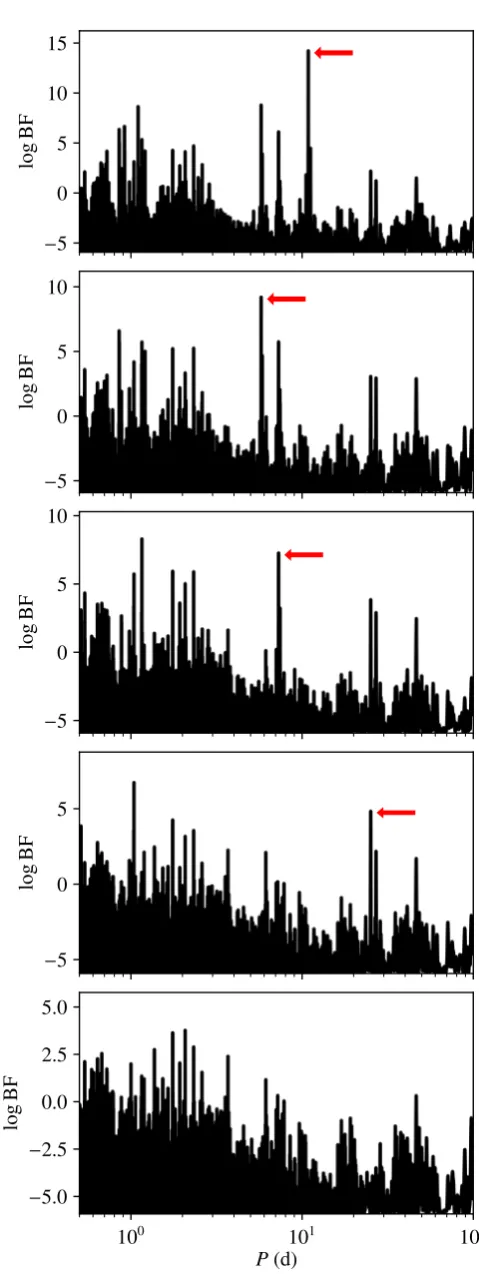
Fig. 4.Periodogram of the RVs at each step of constructing our

Keple-rian model (see Sect.3.3). We highlight (redarrows) the selected period

(highest peak) for each planet: 10.87, 5.76, 7.28, and 25.2 d. We also show (bottom) the periodogram of the residuals. Intermediate values of

Table 2.Evolution of the noise and planetary parameters at each step of the construction of our Keplerian model (see Sect.3.3and Fig.4).

number of planets σJ(m/s) σG(m/s) τG(d) P(d) K(m/s)

0 0.000 1.799 1.035

1 0.000 1.645 0.966 10.866 1.069

2 0.585 1.443 1.568 10.866, 5.760 1.019, 0.798

3 0.653 1.327 1.939 10.865, 5.760, 7.282 0.970, 0.765, 0.666

4 0.651 1.228 1.881 10.865, 5.760, 7.282, 25.197 0.963, 0.773, 0.675, 0.747

planet parameters, by maximizing the likelihood. We then used the Bayesian information criterion (BIC, seeSchwarz 1978)

BIC=2 log_Lmax−plogn (7)

(where pis the number of parameters of a given model) to esti-mate the Bayes factor between the models

log BF(P)=BIC(P)−BICref

2 . (8)

Following Feng et al. (2017), we used these log BF values to draw the periodogram, and we used a threshold at log BF=5 to

add a planet candidate in our model. The main difference in our

approach is that we modeled the correlated noise using a Gaus-sian process (see Sect. 3.2), in contrast to Feng et al.(2017), who used a moving-average model. The complete model (includ-ing all previous planets) was then readjusted by maximiz(includ-ing the likelihood using a downhill simplex algorithm (Nelder & Mead 1965), and we iterated the process. At this stage, we did not al-low eccentric orbits. The successive periodograms thus built are shown in Fig.4. The evolution of the noise and planetary param-eters at each step of the process are detailed in Table2. We find four planet candidates at periods 10.87, 5.76, 7.28, and 25.2 d.

The aliases at one sidereal day (1.16 and 1.04 d) of the two last candidates (7.28 and 25.2 d, respectively) show slightly higher log BF values than the periods we selected. Given that we find a correlation timescale (τG) of about 1-2 days (see Table2), we suspect that periods of about one day are significantly af-fected by the correlated noise, and we considered the candidates at 7.28 and 25.2 d to be more likely than their aliases at one day. However, we cannot rule out any of the possibilities. In order to break the alias at one sidereal day and to better characterize the correlated noise, we would need a dedicated observing strategy with several points per night during several consecutive nights. The signal-to-noise ratio (S/N) and the 43 nights with two points

are not sufficient in this case to apply a dealiasing technique such

as is described inDawson & Fabrycky(2010). As in the case of the logR0

HK index, there does not seem to be a significant signal at the rotation period of the star (about 42 d) in the periodogram of the RV residuals (see Fig.4).

We note that the HD 215152 system was listed in the statis-tical study ofMayor et al. (2011), with a detailed analysis yet to be published. In this previous analysis, only two planets were detected at 7.28 and 10.87 d. We still find these two planets, but we find two other candidates as well (at 5.76 and 25.2 d). How-ever, the number of data points increased greatly since 2011, from 171 to 373 points, the time span increased from 8 to 13 years, and the sampling is better (more nights with two points per night). Since all the candidates have small amplitudes, it is not surprising that some of them were missed in Mayor et al.

(2011). As a comparison, we reran our analysis, but using only the first 171 data points. This analysis differs from the analysis

used byMayor et al.(2011) since we here included the stitching correction, magnetic cycle modeling, and a more complex noise

Table 3.Priors used for the full model sampling.

Parameter (units)

σJ (m/s) |N|(µ=0, σ=5)

σG (m/s) |N|(µ=0, σ=5)

τG (d) logN(µ=0, σ=3)

γi (m/s) U(min=−106, max=106)

A (m/s) U(min=₋103, max=103)

P−1 _{(1/d) U(min=0, max=10)}

K (m/s) U(min=0, max=100)

λ(0) (deg) U(min=0, max=360)

e B(α=0.867, β=3.03)1

ω (deg) U(min=0, max=360)

Notes.(1)_{Kipping(2013) .}

model (Gaussian process). As inMayor et al.(2011), we find the candidates at 10.87 and 7.28 d (with a strong alias at 1.16 d). The 5.76 d signal is just below the detection threshold (log BF<5), and we do not detect the 25.2 d signal. This confirms that the huge observational effort employed since 2011 was essential to

better characterize this system.

3.4. Full model sampling

In order to better determine the orbital architecture of the system, we explored the parameter space of our full model (four planets, offsets, magnetic cycle, and Gaussian process) using an

adap-tive Metropolis approach. The sampling algorithm is described in AppendixA, and the priors are detailed in Table3. We ran two experiments, one with elliptical orbits and one with circular orbits. In both cases, we ran the algorithm for 2,000,000 steps, but only keep the last 1,500,000 steps to compute statistics. Ta-ble4 shows the results of the elliptical fit, while the results of the circular fit are summarized in Table5. In both tables, the uncertainty on the mass of the star (see Table1) is taken into account to derive the minimum masses (msini) and semi-major axes (a) of the planets. Table4clearly shows that the eccentrici-ties cannot be constrained with the current data. This is expected for such low-amplitude signals (K.1 m/s for all four planets).

Table 4.Results of the elliptical fit (see Sect.3.4). Values correspond to the ML, and errors give the 2σinterval.

Parameter (units)

σJ (m/s) 0.632+₋0₀._.189₅₉₅

σG (m/s) 1.262+₋0₀._.303₁₄₅

τG (d) 1.975+₋0₁._.551₀₆₇

γ1 (m/s) −13687.434+₋0₀..175372

γ2 (m/s) −13673.120+₋0₀..901518

A (m/s) −1.504+0.291 −0.508

planet b c d e

P (d) 5.75942+0.00190

−0.00095 7.28345+−00..0086900343 10.86420−+00..0061700500 25.1968+−00..04780526

K (m/s) 0.907+0.151

−0.364 0.608+−00..221315 0.986−+00..300317 0.914+−00..128559

λ(0) (deg) 24.61+28.11

−18.46 −158.04+−3430..5120 98.24−+2820..8307 −37.80+−4233..0437

ecosω 0.354+0.094

−0.417 −0.098+−00..402137 −0.332−+00..440153 −0.167+−00..370200

esinω ₋0.045+0.236

−0.135 −0.131−+00..276151 −0.024+−00..214203 0.048+−00..286264

e 0.357+0.108

−0.351 0.163+−00..160223 0.333−+00..182326 0.173+−00..287169

ω (deg) −7.3+143.2

−143.4 −126.9−+164167..67 −175.8+−151131..56 163.9+−167167..31

msini (m⊕) 1.996₋+00..414746 1.526−+00..792561 2.705−+00..911822 3.467+−02..462133

a (AU) 0.057635+0.000742

−0.000755 0.067399+−00..000898000854 0.08799−+00..0011300115 0.15417+−00..0019900204

Table 5.Same as Table4, but for the circular fit.

Parameter (units)

σJ (m/s) 0.651+₋0₀._.176₆₁₆

σG (m/s) 1.228+₋0₀..338103

τG (d) 1.881+₋0₀..604988

γ1 (m/s) −13687.517+₋00..269274

γ2 (m/s) −13672.936+₋0₀..675730

A (m/s) −1.612+0.380 −0.399

planet b c d e

P (d) 5.75999+0.00157

−0.00175 7.28243+−00..0082700451 10.86499−+00..0056400613 25.1967+−00..04760505

K (m/s) 0.772+0.211

−0.266 0.675+−00..284242 0.963−+00..277317 0.747+−00..275384

λ(0) (deg) 30.43+25.25

−25.49 −156.03+−3728..6651 104.66−+2326..5237 −31.73+−3537..0096

msini (m⊕) 1.819₋+00..501629 1.720−+00..618725 2.801−+00..809923 2.877+−11..063481

a (AU) 0.057638+0.000739

−0.000759 0.067393+−00..000893000860 0.08799−+00..0011300116 0.15417+−00..0019900204

4. System dynamics and stability

The planetary system around HD 215152 is very compact, es-pecially the three inner planets, which exhibit period ratios of

Pc/Pb = 1.26 (close to 5/4) and Pd/Pc = 1.49 (close to 3/2). This compact architecture raises several interesting questions re-garding the dynamics of the system, such as whether the planets are locked in mean-motion resonances, if the observed system is stable, and how the stability of the system depends on the eccen-tricities and the inclinations of the planets. In order to partially answer these questions, we ran three sets of N-body integrations of the system. We used the ML solution of the circular model (see Table5) as a reference and varied the period and eccentric-ity of Planet c to generate three grids of 161x161 (25921) initial conditions. In the first set of simulations (referred to as S90), we assumed the four planets to be coplanar, with inclinations of 90◦_{(m=msini). In the second set of simulations (S30), we} as-sumed the four planets to be coplanar, with inclinations of 30◦ (m =2msini). Finally, the third set (S15) corresponds to

incli-nations of 15◦_{(m≈3.86msini).}

For each initial condition, we integrated the system for 1 kyr using GENGA (Grimm & Stadel 2014), and we assessed the sta-bility of the system using the NAFF stasta-bility indicator (Laskar

1990,1993; Correia et al. 2005). We show the results of these

integrations in Fig.6. In the S90 simulations, where the masses are equal to minimum masses, the system is stable at low eccen-tricities (ec .0.03, see Fig.6top). If the masses are twice the minimum masses (S30, Fig.6center), the system can still be sta-ble, but only at lower eccentricities (ec .0.02). Finally, for the S15 simulations (Fig.6bottom), the system is unstable even at zero eccentricities. We also note in Fig.6that stable orbits that are compatible with the data correspond to a system that clearly lies outside both the 5:4 resonance between Planets b and c and the 3:2 resonance between Planets c and d.

−5 0 5

∆

vb

(m

/

s)

−5 0 5

∆

vc

(m

/

s)

−10 −5 0 5

∆

vd

(m

/

s)

0.0 0.2 0.4 0.6 0.8 1.0

φ −5

0 5

∆

ve

(m

/

s)

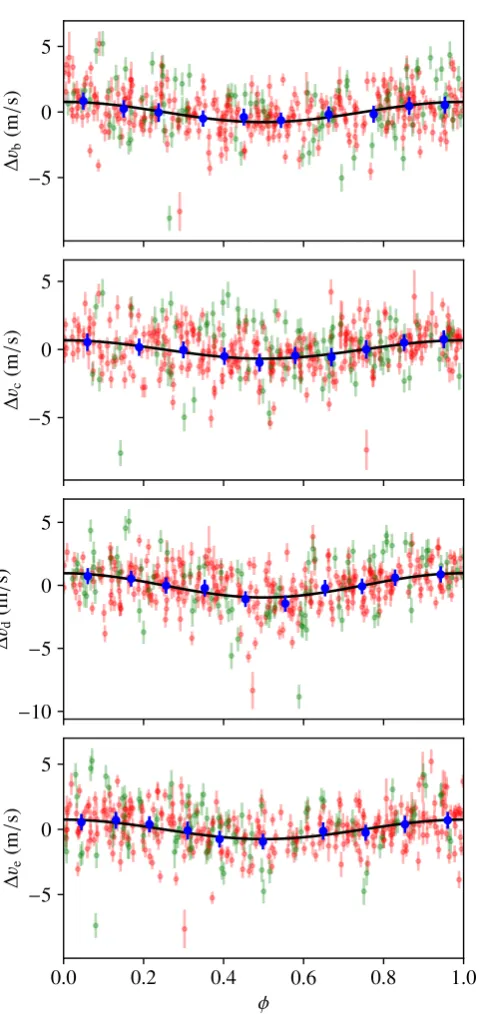
Fig. 5.Phase-folded curve for each of the four planets obtained using

the parameters of the circular ML. Theblackline shows the model.Red

(green) dots correspond to HARPS data taken before (after) the fiber

upgrade.Bluedots show the data binned in phase. For each panel, we

subtracted the Keplerian signal associated with all other planets from the data, as well as the magnetic cycle component and instrumental off-sets.

5. Discussion

We reported the discovery of a compact system of four super-Earth planets around HD 215152. The planets have periods of 5.76, 7.28, 10.86, and 25.2 d, and minimum masses of 1.8, 1.7, 2.8, and 2.9 M⊕(respectively). Planets b and c are close to but outside of a 5:4 mean motion resonance (period ratio of 1.26), and Planets c and d are close to but outside of a 3:2 mean mo-tion resonance (period ratio of 1.49). Owing to the low masses of

0.00 0.02 0.04 0.06

ec

5:4

w

/

b

2:3

w

/

d

S90

0.00 0.02 0.04 0.06

ec

5:4

w

/

b

2:3

w

/

d

S30

7.1 7.2 7.3 7.4

Pc(d)

0.00 0.02 0.04 0.06

ec

5:4

w

/

b

2:3

w

/

d

S15

−10 −8 −6 −4 −2 0

log

10

(

∆

nc

/

T

)(de

g

/

yr

2 )

Fig. 6.Stability analysis of HD 215152 c around the circular ML

solu-tion (see Table5) and assuming planetary inclinations of 90◦_{(top), 30}◦

(center), and 15◦_{(bottom). Blue points correspond to stable orbits, red}

points to unstable orbits, and white points correspond to highly unstable solutions (collision or ejection of a planet during the 1 kyr of the

sim-ulation). The two vertical black lines highlight the 2σinterval for the

period of Planet c. We also highlight the location of the 5:4 resonance with Planet b and the 3:2 resonance with Planet d.

the planets (low S/N), it is very difficult to constrain the planets

eccentricities. However, using N-body simulations, we showed that interesting constraints on the eccentricities and on the in-clinations of the planets could be derived from studying the sys-tem stability. Assuming inclinations of 90◦_{for all the planets, we} find that the system remains stable forec .0.03. If the planets remain coplanar but have inclinations of 30◦ _{(masses of twice} the minimum masses), the maximum eccentricity is about 0.02. Moreover, for a coplanar system with an inclination of 15◦_{, the} system is unstable even at zero eccentricities. Interestingly, these values (ec.0.03) are on the order of magnitude of eccentricities found inKeplermulti-transiting systems that are close to reso-nances (eccentricities inferred using transit timing variations, see

Wu & Lithwick 2013). This is not surprising as the HD 215152

the star on the planets. We note that the bounds we obtain on the eccentricity of Planet c should only be taken as very crude estimates because we did not explore the entire parameter space and only varied a few orbital parameters. A more complete dy-namical analysis is thus necessary to obtain precise constraints on the planet eccentricities and inclinations, but this is beyond the scope of this paper.

Acknowledgements. We thank the anonymous referee for his/her useful com-ments. We acknowledge financial support from the Swiss National Science Foundation (SNSF). This work has in part been carried out within the frame-work of the National Centre for Competence in Research PlanetS supported by SNSF. XD is grateful to The Branco Weiss Fellowship–Society in Science for its financial support. PF and NCS acknowledge support by Fundação para a Ciência e a Tecnologia (FCT) through Investigador FCT contracts of reference IF/01037/2013/CP1191/CT0001 and IF/00169/2012/CP0150/CT0002,

respec-tively, and POPH/FSE (EC) by FEDER funding through the program “Programa

Operacional de Factores de Competitividade - COMPETE”. PF further acknowl-edges support from Fundação para a Ciência e a Tecnologia (FCT) in the form of an exploratory project of reference IF/01037/2013/CP1191/CT0001. RA

ac-knowledges the Spanish Ministry of Economy and Competitiveness (MINECO) for the financial support under the Ramón y Cajal program RYC-2010-06519, and the program RETOS ESP2014-57495-C2-1-R and ESP2016-80435-C2-2-R.

References

Baluev, R. V. 2011, Celestial Mechanics and Dynamical Astronomy, 111, 235 Correia, A. C. M., Udry, S., Mayor, M., et al. 2005, A&A, 440, 751 Dawson, R. I. & Fabrycky, D. C. 2010, ApJ, 722, 937

Díaz, R. F., Ségransan, D., Udry, S., et al. 2016, A&A, 585, A134 Dumusque, X., Lovis, C., Ségransan, D., et al. 2011, A&A, 535, A55 Dumusque, X., Pepe, F., Lovis, C., & Latham, D. W. 2015, ApJ, 808, 171 Fabrycky, D. C., Lissauer, J. J., Ragozzine, D., et al. 2014, ApJ, 790, 146 Farr, B., Kalogera, V., & Luijten, E. 2014, Phys. Rev. D, 90, 024014 Feng, F., Tuomi, M., & Jones, H. R. A. 2017, MNRAS, 470, 4794

Figueira, P., Faria, J. P., Adibekyan, V. Z., Oshagh, M., & Santos, N. C. 2016, Origins of Life and Evolution of the Biosphere, 46, 385

Gaia Collaboration, Brown, A. G. A., Vallenari, A., et al. 2016, A&A, 595, A2 Giguere, M. J., Fischer, D. A., Payne, M. J., et al. 2015, ApJ, 799, 89

Gray, R. O., Corbally, C. J., Garrison, R. F., McFadden, M. T., & Robinson, P. E. 2003, AJ, 126, 2048

Grimm, S. L. & Stadel, J. G. 2014, ApJ, 796, 23

Haario, H., Saksman, E., & Tamminen, J. 2001, Bernoulli, 7, 223 Hastings, W. K. 1970, Biometrika, 57, 97

Haywood, R. D., Collier Cameron, A., Queloz, D., et al. 2014, MNRAS, 443, 2517

Høg, E., Fabricius, C., Makarov, V. V., et al. 2000, A&A, 355, L27 Johnson, J. A., Payne, M., Howard, A. W., et al. 2011, AJ, 141, 16 Kipping, D. M. 2013, MNRAS, 434, L51

Kürster, M., Endl, M., Rouesnel, F., et al. 2003, A&A, 403, 1077 Laskar, J. 1990, Icarus, 88, 266

Laskar, J. 1993, Physica D Nonlinear Phenomena, 67, 257

Lissauer, J. J., Ragozzine, D., Fabrycky, D. C., et al. 2011, ApJS, 197, 8 Lo Curto, G., Pepe, F., Avila, G., et al. 2015, The Messenger, 162, 9 Lovis, C., Dumusque, X., Santos, N. C., et al. 2011, ArXiv e-prints, 1107 Mamajek, E. E. & Hillenbrand, L. A. 2008, ApJ, 687, 1264

Marmier, M. 2014, PhD thesis, Geneva Observatory, University of Geneva Martínez-Arnáiz, R., Maldonado, J., Montes, D., Eiroa, C., & Montesinos, B.

2010, A&A, 520, A79

Mayor, M., Lovis, C., & Santos, N. C. 2014, Nature, 513, 328 Mayor, M., Marmier, M., Lovis, C., et al. 2011, ArXiv e-prints Mayor, M., Pepe, F., Queloz, D., et al. 2003, The Messenger, 114, 20

Metropolis, N., Rosenbluth, A. W., Rosenbluth, M. N., Teller, A. H., & Teller, E. 1953, The Journal of Chemical Physics, 21, 1087

Mowlavi, N., Eggenberger, P., Meynet, G., et al. 2012, A&A, 541, A41 Nelder, J. A. & Mead, R. 1965, The Computer Journal, 7, 308

Noyes, R. W., Hartmann, L. W., Baliunas, S. L., Duncan, D. K., & Vaughan, A. H. 1984, ApJ, 279, 763

Robinson, S. E., Laughlin, G., Vogt, S. S., et al. 2007, ApJ, 670, 1391 Schwarz, G. 1978, The Annals of Statistics, 6, 461

Sousa, S. G., Santos, N. C., Mayor, M., et al. 2008, A&A, 487, 373 Steffen, J. H. & Hwang, J. A. 2015, MNRAS, 448, 1956

Tuomi, M., Jones, H. R. A., Barnes, J. R., Anglada-Escudé, G., & Jenkins, J. S. 2014, MNRAS, 441, 1545

Wu, Y. & Lithwick, Y. 2013, ApJ, 772, 74

Appendix A: Adaptive Metropolis algorithm

In order to explore the parameter space of our model, we used an adaptive Metropolis algorithm inspired byHaario et al.(2001). This algorithm is similar to the classical Metropolis-Hastings al-gorithm (Metropolis et al. 1953;Hastings 1970), except that at each step the proposal is randomly generated around the previ-ous point, using the covariance matrix of all preceding points

(seeHaario et al. 2001).

We additionally included in the algorithm a possibility to go back around an anterior point (not the previous one). This idea is inspired by the tuned jump proposal described inFarr et al.

(2014), and it allowed us to improve the mixing of the chain. We implemented it as follows:

– At each step, there is a given probability (pgo−back=0.01 in

our case) to make a go-back proposal. Otherwise, a classical proposal around the previous point is made.

– In case of a go-back proposal, an anterior point is randomly selected, and a proposal is made around this point (still using the covariance matrix of all previous steps).

– Since the proposal is not symmetrical, and in order to main-tain detailed balance, we computed the forward and back-ward jump probabilities (e.g.,Farr et al. 2014) and took them into account in computing the acceptance probability. – The computation of forward and backward jump

probabil-ities becomes very expensive in computer time when the number of possible anterior points increases. We thus only considered one point over hundred as a possible go-back point (around which the proposal can be made).

We used this algorithm to explore the parameter space for both the elliptical case and the circular case. The results are de-tailed in Sect.3.4(Tables4and5). In order to illustrate the mix-ing properties of our chains, we show in Figs.A.1andA.2the autocorrelation functions of all parameters in both cases. In the elliptical case, the maximum integrated autocorrelation time is 223 (effective sample size of 6,721). This is sufficient to estimate

2σerror bars. In the circular case, the mixing is even better (in-tegrated autocorrelation time of 112, and effective sample size

10

₁₀

₁₀

₁₀

lag

0.0

0.2

0

.

4

0

.

6

0

.

8

1.0

ρ

Fig. A.1.Autocorrelation functions for the 26 parameters of the ellip-tical model, the log likelihood, and log posterior, computed on the last 1,500,000 steps of the Metropolis algorithm. The maximum integrated autocorrelation time is 223, which corresponds to an effective sample size of 6,721.

10

₁₀

₁₀

₁₀

lag

0.0

0.2

0.4

0

.

6

0.8

1.0

ρ