Engineering Entertainment: Adaptive interventions to enhance player engagement in the Interactive Tag Playground

Engineering Entertainment:

Adaptive interventions to enhance player

engagement in the Interactive Tag Playground

Jelle Pingen

Master’s thesis

January 18, 2019

Abstract

The last decade has seen a rise in the use of interactive technology in physical play, with games and interactive installations using players’ body movements as core part of the game experience. This addition of technology gives extra sensing and feedback capabilities to these interactive playgrounds, which enables them to adapt to the current situation and players. This study aims to design and develop an adaptive intervention to enhance player engagement in the Interactive Tag Playground (ITP), an interactive camera-projector system to play the game of tag.

Playing data from the ITP was gathered, and video recordings were analyzed by an observer to mark periods of low engagement during play. This data is used to train a logistic regression model in order to predict the level of engagement during play. The final logistic regression model, using only a subset of features that can be easily retrieved from the ITP, has an F1-score of 0.75. This model, combined with a time frame of 15 seconds and a threshold of 85%, shows promising results at triggering an intervention at appropriate times.

Contents

1 Introduction 9

1.1 Adaptivity in interactive play . . . 10

1.2 Methodology . . . 11

2 Literature review 12 2.1 Goals of Adaptivity . . . 12

2.1.1 Skill balancing . . . 12

2.1.2 Behavior steering . . . 14

2.2 Requirements for adaptivity . . . 14

2.2.1 Sensing . . . 15

2.2.2 Measure of Engagement . . . 15

2.2.3 Measure of Difficulty . . . 16

2.2.4 Player modeling . . . 16

2.2.5 Interventions . . . 17

3 The Interactive Tag Playground 20 3.1 Setup . . . 20

3.2 Adaptivity in the ITP . . . 21

4 Experiment 1 - Data collection and analysis 23 4.1 Introduction . . . 23

4.2 Methodology . . . 23

4.3 Observations . . . 25

4.4 Analysis . . . 25

4.5 Conclusions . . . 31

5 Engagement prediction model 32 5.1 Data . . . 32

5.2 Methodology . . . 33

5.3 Results . . . 34

5.4 Feature selection . . . 35

5.5 Cross validation . . . 37

5.6 Intervention Trigger . . . 37

5.7 Conclusions . . . 39

6 Experiment 2 - Model evaluation 40 6.1 Introduction . . . 40

6.2 Intervention . . . 40

6.3 Implementation . . . 41

6.4 Methodology . . . 41

6.5 Results . . . 42

7 Discussion and limitations 45

7.1 Future work . . . 48

8 Conclusion 50

References 51

List of Figures

1 Flowchart of the game adaptation process . . . 18 2 Left: Disposition of the Kinects and projectors on the ceiling

of the playground. Right: Playing area of the ITP. (Moreno et al., 2015) . . . 20 3 Circles projected on the floor during the tag game. The

or-ange circle denotes the tagger. . . 24 4 Frequency histogram of players’ average heart rate for a single

game . . . 26 5 Heart rate development over time for single player . . . 26 6 Frequency histogram of players’ average heart rate for a single

game after dropping first 120 seconds . . . 27 7 Root-mean-square energy of the sound signal for both low

and not-low engagement in each game. Note that the vertical scales are different per game. . . 28 8 Average player speed (km/h) for each game during low

en-gagement (blue) and not-low enen-gagement (red) . . . 29 9 Illustration of dropped frames around the edges of periods

classified as low-engagement. . . 33 10 Adaptation trigger examples per game . . . 38 11 Implementation of the swag intervention in the adaptive ITP 41 12 Result of GEQR questionnaire scores, per condition . . . 44 13 Average distance between runners and tagger, with and

List of Tables

1 Previous interventions done with the ITP . . . 21 2 Average sound level (RMSE) and Cohen’s d . . . 28 3 Average player speed (km/h) and Cohen’s d . . . 30 4 Average tagger speed at time of tag (in km/h) and standard

deviation (SD) . . . 30 5 Average time between tags (in seconds) for each game . . . . 31 6 Logistic Regression classification metrics . . . 34 7 Logistic Regression confusion matrix (’0’ denotes not-low

en-gagement, ‘1’ denotes low engagement) . . . 34 8 Random Forest classification metrics . . . 35 9 Random Forest confusion matrix (‘0’ denotes not-low

1

Introduction

Play is widely accepted as an essential activity for children, as it provides entertainment, social interaction, as well as physical and cognitive benefits (Barnett, 1990). In the last decade, more technology has been introduced into play, as video games have become a very popular way of playing. How-ever, there has also been a rise in the use of interactive technology in phys-ical play. This has been done in several ways, ranging from interactive toys and attributes to complete interactive installations which use players’ body movements as core part of the game experience (Moreno et al., 2015). True interactive play differentiates from interactive toys in four ways, as defined by Van Delden et al. (2018). Firstly, interactive play systems require explicit body movements for interaction, as opposed to using a controller such as a joystick or mouse. Second, it can enhance the provided feedback in several ways, e.g. by using lights, sounds or movements/vibrations. Thirdly, the interactive play system is able to store a history of states. This means it can, for example, remember where a player has been in order to switch between states or change scores. Lastly, these systems provide the ability to share their state and data between multiple devices, which opens opportunities for new ways of interaction.

These sensing and feedback capabilities enable the use of interactive play-grounds and systems for a number of different goals, as defined by Poppe et al. (2014). First and foremost, interactive playgrounds can provide a fun ex-perience and enhance engagement by presenting novel interaction methods and visualizations. Second, by providing a fun experience, interactive play-grounds further promote physical activity. Through sensing, the system can measure players’ skill and adapt the game accordingly. Third, interactive playgrounds can be employed to stimulate behavior change, i.e. encour-age positive behavior and discourencour-age negative behavior. Fourth, interactive playgrounds can play a role in education and learning. The systems can be adapted to support a certain theme or learning goal. Finally, interactive playgrounds may even provide opportunities for diagnosis. Using automatic sensing, players’ behavior can be analyzed and possibly spot any abnormal-ities.

Kajastila et al. (2016)). The system uses a depth camera and projector to help climbers by projecting possible routes, giving video feedback or even play small games. Their study has shown that these augmented visuals can increase the diversity of movements and challenges, by steering play-ers to unexpected directions. Based more on traditional children’s play is the interactive playground developed by Tetteroo et al. (2011). Their sys-tem tracks players’ positions with an infrared camera which films reflective markers attached to the players’ heads. Next to that, Sun SPOT sensors were used to track small foam balls. A projector mounted on the ceiling can project visualizations on the floor. This playground allows for open-ended play, where players can create and interact with several projected shapes. Similar to this setup, are a number of commercially available interactive play systems. Most of them employ a similar setup of a (depth-)camera to track players and a projector to project visualizations on the floor, like the BEAM from EyeClick1 and the MotionMagix box2. LumoPlay3, for example, only provides the software that can be used with your own projector/camera setup.

1.1 Adaptivity in interactive play

The first three chapters of this thesis are largely based on the ‘research topics’, a preliminary (literature) study conducted as an exploration of the research area (Pingen, 2017). This preliminary study mainly focused on the possibilities of adaptivity in the Interactive Tag Playground (ITP), an inter-active playground setup at the University of Twente. This setup is further discussed in section 3. Previous interventions in the ITP were analyzed, along with different methods to make the ITP more adaptive. Because of its availability, it was decided to use the ITP as main instrument for this research. Focusing specifically on player engagement in the ITP appeared to give the most interesting options for adaptive interventions. Previous research with children in the ITP has shown that player engagement de-creases after about 90-100 seconds. This is a good opportunity for the ITP to adapt to and automatically intervene, in order to restore engagement. Furthermore, to circumvent any issues with tracking issues in the ITP, the system should look at a global (combined) model of player engagement in-stead of each individual player. The preliminary study lead to the following research question, which form the basis for this thesis:

• How to create adaptive interventions for the Interactive Tag Play-ground to enhance player engagement?

1

http://www.joinbeam.com/, last accessed 18-06-2018

2

http://www.motionmagix.com/, last accessed 15-06-2018

3

To answer this main research question, the following two sub-questions were devised:

1. How can the ITP sense or detect when to intervene?

2. What is the effect of an adaptive intervention?

1.2 Methodology

When trying to solve these questions, one has to take the requirements for the intervention into account. The intervention should preferably be simple and robust, have a clear and great effect on the players, and be easy to make adaptive. Next to this, the limitation of the system should be taken into account. Previous research with the ITP has shown that occasionally a ‘track switch’ occurs, which means that the tracking system assigns the wrong ID to the wrong player. This may result in incorrect adaptations. To solve such issues, the adaptive system only looks at a global model of player engagement.

The goal of this research is thus to develop an adaptive intervention, which can enhance player engagement in the ITP. In order to do so, the approach is divided into three steps:

1. Gather data and recordings of play sessions in the ITP. In order to create an adaptive intervention, the system must be able to distinguish between a high and low level of engagement. Therefore, the recorded play sessions should include both a high level of engagement as well as (part of) sessions with a low level of engagement.

2. Create a model of player engagement in relation to playing in the ITP. Using the data gathered in the previous step, determine which elements indicate engagement levels and should thus be the actual trigger for the intervention. This might be a combination of different types of player data, such as amount of movement, sound, game speed or even the players’ heart rate.

2

Literature review

In order to properly design an adaptive intervention, it is important to discuss the previous research in this area. The following chapter provides an overview of the different adaptive systems that have been developed, which problems they aim to solve and what is needed to create such adaptive systems.

2.1 Goals of Adaptivity

As shortly mentioned before, by making interactive playgrounds adaptive they can provide an engaging and entertaining experience, while actively promoting or discouraging certain types of behavior. Ambient games have been shown to benefit from behavioral analysis to adapt the game (Schouten et al., 2011). Instead of analyzing the data afterwards, information can be processed during play, which makes new types of interactions possible (Moreno, 2016). By adapting the game mechanics during play, an interactive playground can challenge the players based on their personal skill level, thus making the game more fun to play. Next to that, adaptive playgrounds can even be used to encourage positive social behavior.

2.1.1 Skill balancing

Games, and thus interactive play systems, become boring when they are too easy and frustrating when the difficulty is too high, which might lead to a lower level of engagement. In order to account for this problem, games usu-ally give the player the option to select a difficulty level (Lopes and Bidarra, 2011). However, the chosen challenge level is static, and does not depend on the actual player performance. This may lead to a mismatch between player skill and game difficulty, for example when players incorrectly clas-sify themselves. Therefore, many game designers aim to adjust the game difficulty during the play. This is also known as Dynamic Difficulty Adjust-ment or Dynamic Game Balancing. Even in multiplayer games, similar to a handicap in the game of golf, some players can be given an advantage or disadvantage based on their skill level in order to even the playing field. This can be done for each (sub)set of skills: e.g. running speed, strength, agility, etcetera. This can increase challenge for the player, which in turn leads to a higher level of engagement. However, proper dynamic game balancing is not easy to accomplish. Schell (2008) defines three problems with dynamic game balancing:

2. It is exploitable. When players realize the game will get easier if they play badly, they might play badly on purpose in order to win or complete a challenge. This migh defeat the purpose of an adaptive difficulty (i.e. players are not challenged anymore).

3. Players improve with practice. If enemies get easier to beat each time you’re defeated by them, the game loses the aspect of challenge and the pleasure it gives players of mastering that challenge.

The first might not be too much of a problem for interactive playgrounds. These systems are usually not designed to fully immerse the players in a vir-tual world, since they are mostlyaugmenting the real world. The other two problems mentioned above should definitely be considered while designing the adaptive system for such a playground. Exploitation, for example, might be hard to detect without an external (human) observer. Next to that, it is important to keep the challenge at an adequate level in order not to lose engagement.

Skill balancing is not new, as extensive has been done on this subject. For example, Andrade et al. (2006) developed an intelligent adaptive agent for a real-time fighting game, using reinforcement learning. This agent can choose between actions with high or low expected performance. For exam-ple, if the game level is too hard, the agent chooses a sub-optimal action, and progressively less optimal actions until its performance is as good as the player. Similarly, if the game level is too easy, it will pick a progres-sively better action until it matches the player’s skill. Their study shows that this adaptive approach has the best result compared to other adaptiv-ity approaches: it can adequately deal with players of different skill levels, providing a challenging opponent for each. Next to that, it also provided the highest user satisfaction. Their approach is similar to thedynamic scripting

technique by Spronck et al. (2003). Dynamic scripting uses an adaptive rule-base to control the opponent AI in a game. The rulerule-base’s weights are then updated based on the success or failure rate of a particular rule. Dahlbom (2004) proposes a new, adaptive structure for this approach, employing a goal-rule hierarchy. In this case, rules are viewed as a strategy to reach a higher-level goal. The system is adaptive by adjusting the probabilities of selecting each rule. This allows the AI to make strategic choices and in-crease the challenge for the player when needed. Results have shown that this updated dynamic scripting algorithm can be more effective, and can re-adapt quicker than the original algorithm.

to win more), it reduced the engagement for the higher-skilled player. Jog-ging over a Distance, as developed by Mueller et al. (2012) aims to balance exertion in jogging pairs. The joggers can hear the audio of their co-located jogging partner. This audio is positioned in a 2D space around the joggers head, based on the difference of the relative heart rates. If one jogger’s heart rate is relatively high, the other jogger would hear him ‘in front’ of him, and vice-versa. This allows people with different skill levels to run together in a balanced way. Also the Adaptive Circles by Van Delden et al. (2014) balance players of different skill levels. In a game of tag, players of a higher skill level (i.e. those who are never tagged), are made easier to tag. This evens out the playing field to some extent.

2.1.2 Behavior steering

As mentioned before, interactive play systems can be employed to stimulate behavior change. In order to encourage positive social behavior, the system needs to be able tosteer the player’s behavior. In this case, steering refers to “introducing interactions or gameplay elements that change in-game physi-cal play behavior towards a desired direction”. This is different from more traditional persuasion methods, as it does not aim for long-term behavior change outside of the game (Van Delden et al., 2018). It also does not constrain behavior by hiding certain options or enforcing a specific type of interaction. In contrast, it tries to influence player activity, such as how and where they move or what type of interaction they perform.

This can be done by changing (adapting) the game mechanics. Naturally, the best way to accomplish this is to employ a (slightly) different set of game mechanics or feedback tailored towards each specific player (Poppe et al., 2014). As one player might not be as involved as the others, the system could give them a more prominent role. As mentioned previously, steering gameplay also allows players of different skill levels to play together (such as done by Van Delden et al. (2014)). Next to that, it can also be employed to increase physical exertion and activity (Moreno, 2016). For example, Landry and Pares (2014) show that they are able to control physical activity of the players by changing the interaction tempo of the game (i.e. the pace of gameplay).

2.2 Requirements for adaptivity

two steps, required to ensure that game adjustments induce the personalized player experience, are essential but still form a major challenge.

2.2.1 Sensing

To correctly interpret player behavior, sensors are needed that can capture a player in sufficient detail (Greenberg et al., 2011). Currently, most inputs are low-fidelity, limited and include some level of noise. It is therefore a challenge to design a robust interactive system with such data. More importantly, these sensors need to be embedded into the environment without hindering or distracting players (Moreno, 2016). For example, equipping children with microphones might restrict their movement, or at the very least make them

aware of the microphones, which in turn might lead to different behavior. In the case of interactive play systems, the tracking should have a high temporal and spatial resolution. This means it should react quickly and accurately: it should be accurate enough to distinguish different players and possibly even different types of movement. If the system wrongly identifies players or behavior, it means it will now adapt to the wrong action. Moreover, the study of Nijhar et al. (2011) shows that a higher accuracy of movement recognition leads to a higher level of immersion for the players.

2.2.2 Measure of Engagement

In order to increase player or group engagement, the level of engagement needs to be measured accordingly. However, it must be noted that inter-preting behavioral cues only indirectly observes actual player experience (Yannakakis et al., 2013). For example, a player who has only little inter-action with the system (i.e. is not moving much) may be either bored or actually thoughtful and captivated. As such, behavioral metrics can only approach the likelihood of experience.

Bianchi-Berthouze discusses the role of body pose and motion in detect-ing user engagement, by usdetect-ing body trackdetect-ing systems such as the Kinect (Bianchi-Berthouze, 2012, 2013). Changes in body movement entropy can show how the player is appropriating the game control, which might be an indicator of user engagement. Players enter a vicious circle of sorts; they are more affected as they move more, which in turn makes them want to move even more. Monitoring movement entropy might, therefore, be a good indicator of user engagement, either personal or for the group of players as a whole. Measuring group engagement might also give a way to detect outliers: players that are not really engaged and might need some extra stimulation to join the play.

move-ment, identity (who is playing) and location (Greenberg et al., 2011). The physical arrangement of groups, how players position themselves in relation to others, can be an indicator of engagement. For example, shy players might hide behind others, or very engaged players might hide behind other players to use them as a ‘human shield’. This physical group-arrangement might therefore be an indicator of the relation between players.

2.2.3 Measure of Difficulty

Relating to the previously discussed ability of the system to ‘identify what triggers the need for adjustments’, it can be hard to assess whether a game is too difficult for a player or not. Hunicke and Chapman (2005) try to predict this level of difficulty by determining flailing behavior. To do this, they look at the inventory of the player. First, the overall flow (input and output) of inventory items is modeled. Using this inventory flow, and an estimation of the upcoming damage to be received, it is possible to predict a shortcoming in the inventory. When this is detected, the player will probably not complete the level or task and most likely fail. When this is detected, the game can adapt by, for example, spawning more items or decreasing the damage of an incoming attack.

Bailey and Katchabaw discuss several factors that need to be taken into account in order to determine when to adjust game difficulty (Bailey and Katchabaw, 2005): the player’s skill level, their success/failure rate for var-ious gameplay elements, and the player’s general type, motivations, frustra-tion tolerance, and emofrustra-tional state. The player’s skill and success/failure rates are naturally tied to the particular game or gameplay elements. There are multiple metrics that can be measured from the game itself, for exam-ple the number of attempts before success, time to comexam-pletion or amount of damage taken per level. Using these metrics, it is possible to determine when a player is encountering difficulty with a certain element of gameplay. In these cases, the game or interactive play system can adapt that particular game-element, or support the player in other ways.

2.2.4 Player modeling

the player, one of the pre-defined game adaptations can be utilized, tai-lored to that specific playing style. This process consists of three phases:

observation, classification and adaptation. The observation phase can be automatically done by the interactive play system’s sensors. The classifi-cation phase is a difficult problem. First, different classes of players must be defined. Consecutively, an on-line classifier must be constructed which can classify players to one of the defined classes in (near) real-time. The adaptation phase is then merely choosing the right (pre-defined) parameters based on the classification. For example, idle players might be encouraged to become more active by choosing a higher game speed. With a working classifier, one can even analyze different game strategies employed by the players, and see which one works best. Going even further, the playground can potentially steer the players towards the optimal playing strategy.

Besides player classification based on their behavior, it is also possible to create unique, personal profiles tailored towards a single user. For each person, the system would store their personal preferences and behavior, as opposed to mapping them to a set of pre-defined profiles. This could lead to a highly optimized and adapted system. However, constructing such user profiles is a hard problem. The system would need a way to learn that user’s behavior. Next to that, it would need a way to detect which user is playing. This can be done either automatically (e.g. using cameras to detect and identify different players), or by making the players log-in before the game (and log-out afterwards). The latter method has a downside that players are not able to simply walk in and out of the playground whenever desired, as is common in regular playgrounds.

2.2.5 Interventions

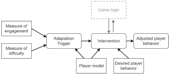
In order to design and develop a fully adaptive system, an inventory of different kinds of interventions is needed. Such an ‘intervention’ is a set of game mechanics or interactions designed to either stimulate or discourage a certain type of behavior. This means that (ideally) for each type of possible (undesired) behavior or interaction in the game, an intervention needs to be designed, leading to a database of interventions. This can be a very time-consuming process, as each intervention needs to be studied and evaluated to make sure it has the right, desired, effect on the players.

model into account and the expected outcome behavior when selecting an intervention. This is a continuous process, which can be roughly modeled as outlined in figure 1.

Figure 1: Flowchart of the game adaptation process

The game adaptation process is, for the most part, separate from the game logic. This separation between game logic and adaptation logic can also be found in the ALIGN system as developed by Peirce et al. (2008). Each intervention, or Adaptive Element (AE) as they call it, is pre-designed and annotated with metadata which describes in which game settings it can be used and what the outcome of its use would be. A separate process analyzes game events and translates this to the appropriate AE, taking the player model into account. This separation of adaptation logic and game logic allows for greater independent control over each element.

sensors in the ITP.

3

The Interactive Tag Playground

The Interactive Tag Playground (ITP) is an interactive playground, aug-mented with sensors and projectors in order to enhance game play (Moreno et al., 2015; Van Delden et al., 2014). It was developed by the Human-Media Interaction group at the University of Twente to conduct research on interactive play.

3.1 Setup

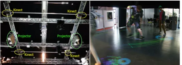
The ITP consists of four Kinect 3D-cameras and two projectors. The four Kinect cameras are mounted on the ceiling in a grid-like pattern, 4 meters apart. The two wide-angle projectors are also mounted on the ceiling, 4 meters apart, displaying visualizations on the floor. Together, they cover an area of about 5.3 by 5.3 meters. Figure 2 shows the setup of the interactive playground. Only the depth images from the Kinect cameras are used, since the projected visualizations would be picked up by the color cameras as well. These depth images are filtered to remove noise and thresholded in order to detect players. The detected positions are then mapped from local Kinect coordinates to global coordinates. The cameras have a slight overlap, thus in order to prevent duplicate detections, detections closer than 50 centimeters are merged together. Based on the detections, the movement of each player is logged using a real-time tracker. This tracker uses Kalman filters to estimate the locations for each player in each frame.

Figure 2: Left: Disposition of the Kinects and projectors on the ceiling of the playground. Right: Playing area of the ITP. (Moreno et al., 2015)

automati-cally chosen as tagger by the system. When the tagger tags another player, their roles, and thus the color of their circles, switch. In contrast to tradi-tional tag, players do not have to physically touch, but can tag each other by making their circles overlap. A sound effect is played to indicate the tag event. Next to that, a cooldown period of two seconds is enforced, during which the tagger cannot tag back the previous tagger. This is visualized by making the previous tagger’s circle semi-transparent. In case the tagger leaves the playing area (or is lost by the tracking system) for two seconds, another player is randomly assigned as tagger.

Since the ITP is equipped with multiple sensors, it is possible to au-tomatically detect and analyze different cues of player behavior. The ITP currently tracks the player position, movement (speed and direction, which can be deducted from the position), tag events and current game state (e.g. who is tagger or runner in the game of tag). All this information is stored and can be used for analysis, either afterwards or possibly even during play.

3.2 Adaptivity in the ITP

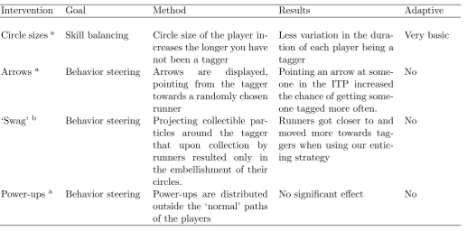
A number of different interventions have already been implemented and re-searched using the ITP. However, the interventions were not all fully adap-tive. Table 1 shows the previously implemented interventions in the ITP.

Table 1: Previous interventions done with the ITP

Intervention Goal Method Results Adaptive

Circle sizesa Skill balancing Circle size of the player in-creases the longer you have not been a tagger

Less variation in the dura-tion of each player being a tagger

Very basic

Arrowsa Behavior steering Arrows are displayed, pointing from the tagger towards a randomly chosen runner

Pointing an arrow at some-one in the ITP increased the chance of getting some-one tagged more often.

No

‘Swag’b Behavior steering Projecting collectible par-ticles around the tagger that upon collection by runners resulted only in the embellishment of their circles.

Runners got closer to and moved more towards tag-gers when using our entic-ing strategy

No

Power-upsa Behavior steering Power-ups are distributed outside the ‘normal’ paths of the players

No significant effect No

In order to detect and decidewhen adaptivity is required, the ITP needs to sense when the engagement appears to be low. Therefore, in order to properly apply such adaptivity, it is required to do some behavior analysis or activity recognition.

4

Experiment 1 - Data collection and analysis

4.1 Introduction

In order to make the system adaptive, it needs to be able to distinguish between high and low engagement during play. Previous research with the ITP resulted in the creation of the ‘Play Corpus’: a dataset of children playing tag. Unfortunately, the playing time in this dataset was deliberately kept short so the children would not get too bored. This means that there are very few periods of low engagement in the dataset. Furthermore, it would be hard to visually detect engagement, as there is no video of the players’ facial expressions. Therefore, new data would have to be gathered which includes periods of both high and low engagement. To make sure that the new dataset would indeed include periods of low engagement, it was decided to let the game run for a longer time. It was expected that by letting the players play for a longer time, eventually an engagement dip would occur as players get bored.

4.2 Methodology

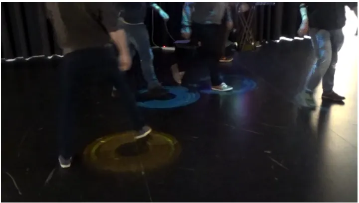
Five games were played in the ITP, each game consisting of four players, giving a total of 20 participants. Participants’ age ranged from 16 to 28 (median: 17), with 15 males and 5 females. Each game had a duration of 10 minutes, with about 13 seconds of introductory audio at the start. Play-ers were instructed to stay within the designated play area until the game was finished. Before playing, each player was also outfitted with a Scosche Rhythm+ heart rate monitor armband4, which was connected through Blue-tooth to an Android smartphone running the Sport Gear Tracker5 applica-tion. Figure 3 shows players playing a game of tag in the ITP.

A Kinect 2 sensor was placed on a tripod (putting the sensor at around 2 meters high) next to the playing area to capture sound. This sensor was chosen due to its multi-array microphone setup and ambient noise cancel-lation abilities. A separate video camera was used to capture video of the play area. During play, the ITP automatically logs players’ positions, role (tagger or runner) and tag events. An observer annotated any anomalies during the game, such as heart rate armbands getting loose, track switches, etcetera. Afterwards, the video recordings were re-watched and periods of low engagement were marked.

4

www.scosche.com/rhythm-plus-heart-rate-monitor-armband, last accessed 12-01-2018

5

Figure 3: Circles projected on the floor during the tag game. The orange circle denotes the tagger.

Data collection

With the setup as described, for each game a number of different types of data is collected:

Heart rate: The Scosche Rhythm+ heart rate armband, connected to the Android app, records the player’s heart beat every second, in beats per minute.

Sound: The Kinect v2 has a four-microphone array, which detects audio input in an angle of 100◦around the sensor. It outputs a 32-bit audio stream, sampled at 48 kHz.

Position & role: About 3 times per second, the ITP logs for each player their position, as well as their current role in the game (tagger or runner). A median filter of 5 frames is applied to the x- and y-position separately to filter out noise. From this position data, other data such as player speed can be derived.

Tag events: Every time a tag event occurs, the ITP logs the timestamp (in milliseconds since the game started) at which it happened, as well as which player was tagged by who.

4.3 Observations

From the observations, a couple of things could be noted. Firsly, it appears that ‘track switches’, where players are assigned the wrong circle after com-ing too close to each other, are almost no issue for the game. These track switches would occur a couple of times per game. Players quickly learned to deal with it, and some even used it to their advantage by clinging onto other people so their own circle would disappear. The same can be said for the tracker performance: the projected circles would sometimes lag behind the player a bit depending on the their speed, but again players quickly adapted their playing style to make use of this mechanic. No real problems with these ‘bugs’ were expressed by the players.

4.4 Analysis

After collecting all the data, it is possible to make a comparison between periods of low engagement and the rest of the game. In the following section, each type of data is analyzed to find possible indicators of low engagement. For this analysis, the SciPy6 package for Python was used, which contains several tools for data analysis and statistics.

Heart rate

Heart rate is a generally accepted indicator of a person’s physical effort (Achten and Jeukendrup, 2003). Physical exertion will lead to an increase in heart rate. Therefore, heart rate might be a good indicator of engagement in the ITP.

Unfortunately, the heart rate sensors that were used were not completely fool-proof. One player had issues with correctly fastening the sensor to his arm, which resulted in the armband shifting and coming loose during the game. For another player in a different game, it was noted afterwards that apparently the sensor had some problems with connecting to the Android application, leading to missing heart rate readings. For these two players, the heart rate data was discarded, resulting in 18 correct heart rate readings which could be used for analysis.

Comparing exercise intensity between individuals is often done by using a percentage of the person’s maximal heart rate (HRmax), as this maximal

heart rate appears to decrease with age. The most commonly used equation isHRmax = 200 - age, but it is debated how accurate this is (Tanaka et al.,

2001). Combined with the fact that the age range of the participants is relatively small, it was decided to just use the absolute heart rate instead.

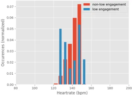
However, simply taking the heart rate for the whole game yields skewed results, as can be seen in figure 4. The histogram shows a lot more

occur-6

rences in the lower regions (<140 bpm) for not-low engagement. This is due to the way a person’s heart rate changes during exercise. Figure 5 shows a single player’s heart rate during the game. As can be seen, the heart rate keeps rising for about 150-200 seconds (from 75 bpm to 175 bpm), after which it only fluctuates around 150-175 bpm. This effect is visible for all players. This, combined with the fact that low engagement generally occurs in the second half of the game, skews the analysis quite a bit.

Figure 4: Frequency histogram of players’ average heart rate for a sin-gle game

Figure 5: Heart rate development over time for single player

To solve this problem, the first two minutes were dropped, which removes the rise in heart rate at the start of the game. Dropping the first two minutes of heart rate data and averaging them per game, yields a histogram as can be seen in figure 6. Looking at the figure, there seems to be a visible difference between low- and high engagement. Low engagement periods have more occurences in the 120-140 bpm region, while high engagement generally occurs more often in the region of 140-150 bpm. However, no statistical significant difference could be found between the two conditions (meanLow engagement = 149.4, meanHigh engagement = 154.6, p-value = 0.28).

Sound

The loudness of an audio signal closely corresponds with the energy of that signal (the total amplitude of the signal), which is defined as:

energy=X

n

Figure 6: Frequency histogram of players’ average heart rate for a single game after dropping first 120 seconds

The root-mean-square energy (RMSE), which will be used as indicator of ‘loudness’ in the analysis is thus defined as:

RM SE =

s

1

N

X

n

|x(n)|2

For the analysis of the sound files, the LibROSA7 library for Python was used, which can compute the RMSE for each frame in the recorded audio file. It is expected that the energy will be lower (i.e. players are more quiet) during low engagement periods.

As can be seen in figure 7, during periods of low engagement (the blue bars) there are relatively more occurrences in the lower end of the spectrum for most games. This might indicate that players are quieter when the engagement is low, which would be consistent with the observations. During high engagement, players tend to shout to each other, laugh more often, and their shoes make more noise on the floor.

Due to the large number of samples (over 25.000 per game), when con-ducting a t-test on the mean RMSE the p-value will quickly go to zero, in this case with results in in the order of p=10-20. Therefore, instead of relying on this extremely low p-value, the effect size is analyzed instead by means of Cohen’s d. Cohen’s d is the difference between the two sample means, divided by the pooled variance. A score of 0.2 is considered a ‘small effect’, a score of 0.5 a ‘medium effect’ and 0.8 a ‘large effect’. As can be seen in table 2, the effect size is very small with an average of 0.12 over all games.

7

Figure 7: Root-mean-square energy of the sound signal for both low and not-low engagement in each game. Note that the vertical scales are different per game.

Game 4 shows the largest effect, but with d=-0.249 this is still considered relatively small.

Table 2: Average sound level (RMSE) and Cohen’s d

Game Low engagement mean

Not-low en-gagement mean

Cohen’s d

1 1.013 0.798 0.148

2 0.892 1.005 -0.085

3 0.399 0.470 -0.087

4 0.886 1.320 -0.249

5 1.166 1.242 -0.049

Speed

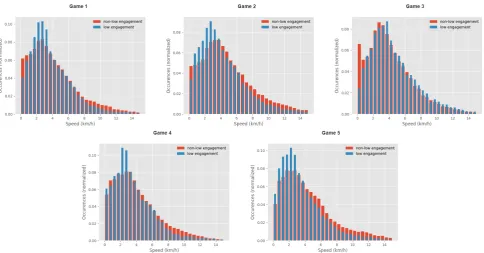
frequency histograms for player speeds, for both low engagement and not-low engagement.

As can be seen in the figure, there is not much difference in player speed between low engagement and not-low engagement. In game 1, 2 and 5, the histogram for low engagement (blue bars) seems a bit shifted to the left: higher speeds (>6 km/h) occur less, whereas lower speeds (<4 km/h) occur more. Interestingly, standing (almost) still (speed <0.5 km/h) appears to happenless during low engagement.

Figure 8: Average player speed (km/h) for each game during low engagement (blue) and not-low engagement (red)

As with the sound analysis, the speed data also has a lot of samples (around 15000) for each game. Thus, again the Cohen’s d is calculated to measure the effect size. Table 3 shows the Cohen’s d for each game. With an average of d=0.153 over all games, the effect is considered to be low. Moreover, the effect is not even in the same direction for all the games: in game 3 and 4, the speed ishigher on average during low engagement.

Tag speed

Table 3: Average player speed (km/h) and Cohen’s d

Game Low engagement mean

Not-low engage-ment mean

Cohen’s d

1 3.423 3.703 -0.154

2 3.794 4.300 -0.267

3 4.081 3.703 0.207

4 3.712 3.485 0.127

5 3.782 3.802 -0.010

will likely follow. As such, the speed of the tagger might say something about engagement. From the observations it was noted that during low engagement, taggers would make low effort to tag others, usually slowly walking around until (s)he could tag someone. Therefore the speed of the tagger at the time of tagging is analyzed.

First, the timestamp from the logged tag events are taken. Then, from the previously discussed player speeds, the speed of the player who was the tagger at that time is taken. These speeds are then averaged for both low-engagement and the rest of the game. The results can be seen in table 4. For each game the tagger’s speed is lower when the engagement is low, as expected. For game 3 and 4, this shows a trend (p<0.1) but also game 5 shows a high difference between low engagement or not. These results show that the speed of tagger at the time of tagging can be an indicator of low engagement.

Table 4: Average tagger speed at time of tag (in km/h) and standard devi-ation (SD)

Game Low engagement mean (SD)

Not-low engage-ment mean (SD)

p-value Observations

1 7.81 (3,6) 7.94 (2,7) 0.79 (83,154) 2 7.51 (2,6) 8.10 (2,8) 0.30 (39,111) 3 5.52 (2,7) 8.00 (2,6) 0.051 (9,83) 4 5.03 (2,4) 8.26 (2,5) 3.74e-5 (19,119) 5 8.37 (3,1) 9.48 (3,1) 0.14 (29,134)

Tag frequency

Another hypothesis was that the higher the engagement, the more often players would tag each other. As players would become more bored and engagement drops, they would not put in as much effort to tag another player, thus resulting in a lower tag frequency.

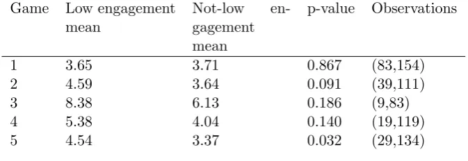
can easily be retrieved. Table 5 shows the average time between tags for each game for periods of low engagement and not-low engagement. In the Observations column, the first number is the number of tags that happened during a period of low engagement, the second number are the amount of tags during the rest of the game. Except for game 1, the time between tags is higher when the engagement is low. This again shows a trend (p <0.1) for game 2 and 5. Game 3 shows the largest difference (8.38 seconds versus 6.13 seconds), but with a p-value of 0.186 cannot be considered significant. This is likely due to the relatively low number of observations (only 9 tags occurred during low engagement, 83 tags during the rest of the game). The time between tags appears to be a promising indicator of low engagement.

Table 5: Average time between tags (in seconds) for each game

Game Low engagement mean

Not-low en-gagement mean

p-value Observations

1 3.65 3.71 0.867 (83,154) 2 4.59 3.64 0.091 (39,111)

3 8.38 6.13 0.186 (9,83)

4 5.38 4.04 0.140 (19,119) 5 4.54 3.37 0.032 (29,134)

4.5 Conclusions

From the analysis, it appears that mainly ‘tagger speed’ and ‘tag frequency’ might be good indicators of low engagement, since they show the most sig-nificant difference between high- and low-engagement periods. As expected, both of them are lower during low engagement, meaning that taggers tag people less often and do so with a lower speed. Contrary to expected, this same difference could not be found for the average speed ofall players. Es-pecially heart rate is difficult to use as indicator of low engagement. Players’ heart rates start rising at the start of a game, until they reach a more stable value. Next to that, it is difficult to correlate heart rate with engagement levels. This is also shown by Yannakakis et al. (2008), who reach a 64% accuracy on children’s preferences in interactive playgrounds, by using mul-tiple heart rate features in a complex neural network.

5

Engagement prediction model

After manual statistical analysis has shown promising indicators of low en-gagement, a model is created in order to try to predict low engagement accurately in new games. Using the previous analysis as a starting point, a machine learning classifier was implemented and used as a predictor.

5.1 Data

The complete dataset consists of five games of four players each. Each game had a duration of 10 minutes. During each game, the following data was recorded: position of each player (about 3 times per second), player role (tagger or runner), tag events, heart rate of each player and global sound level. From these recordings, the following data features were derived:

• Seconds since start: Amount of time the current game is running (in seconds)

• Sound level: Captured global sound energy (total magnitude of the signal)

• Time between last two tags: Amount of time (in seconds) between the last two tag events

• Tagger speed: Speed (in km/h) of the tagger at the last tag event

• Speed: Average speed of the four players, in km/h

• Heart rate: Average heart rate of the four players, in beats per minute

• Heart rate variability: Average heart rate variability of the four players over the last five seconds

This results in a relative score of the feature, compared to normal play (the ‘baseline’ value).

Next, the data was split into frames of 0.5 seconds, where the average value for each feature during this time frame was taken. Each frame was then assigned a label (low engagement or not) based on earlier observations. In order to account for observer accuracy, frames within a second of the edges of a period of low engagement were dropped, as illustrated in figure 9. Each vertical bar represents a frame of 0.5 seconds, the frames classified as low-engagement are colored green. The red area shows the frames that are dropped. This resulted in a final dataset of 6522 frames with 7 features. Of these 6522 frames, around 23% is labeled as low engagement.

Figure 9: Illustration of dropped frames around the edges of periods classi-fied as low-engagement.

5.2 Methodology

only slightly outperforming randomly guessing. Therefore, under-sampling is first applied to the dataset, by using Scikit-learn’s default ‘RandomUnder-Sampler’ method. The under-sampling method randomly picks frames from the majority class (not-low engagement) to approximately balance the two classes. This results in a dataset of 3032 frames, with a ratio of 46/54 low-engagement/not-low engagement.

This balanced dataset is split into 75% training set and 25% test set after shuffling. The dataset is shuffled because frames labeled as low engagement are always next to each other, leading to an imbalanced training and/or test set. Next, both the Logistic Regression classifier and Random Forest classifier are fitted to the training set, using the features as described earlier.

5.3 Results

Using all 7 available features, the initial classifiers seem to perform quite well. As can be seen in table 6 and table 7, the logistic regression classifier has an average F1-score of 0.78. The precision for the low-engagement class is a bit lower than for the non-low engagement class, but this is reverse for recall.

Table 6: Logistic Regression classification metrics

Class Precision Recall F1-score N Not-low engagement 0.83 0.73 0.78 406 Low engagement 0.73 0.83 0.78 352

average/total 0.78 0.78 0.78 758

Table 7: Logistic Regression confusion matrix (’0’ denotes not-low engage-ment, ‘1’ denotes low engagement)

Actual

v

alues

Predicted values

0 1

0 298 108

1 60 292

of the model. Looking further into some of the decision trees of this random forest classifier, it appears that they are indeed overfitting mainly on the ‘Seconds since start’ feature. The classifier learns the exact timings of the periods of low engagement in the dataset. While this yields a very high accuracy score, this cannot be generalized over future games as timings will be different. Countering overfitting by limiting, for example, the maximum tree depth or minimum samples required for a split or a leaf reduces the score on the test set, but the model still tries to capture the exact training values.

Therefore, logistic regression seems to be the better choice for the prob-lem. A linear relation between the features and classes (low engagement or not) is a logical fit and less prone to overfitting than the way the decision trees try to capture the data.

Table 8: Random Forest classification metrics

Class Precision Recall F1-score N Not-low engagement 0.96 0.92 0.94 406 Low engagement 0.91 0.96 0.93 352

average/total 0.94 0.94 0.94 758

Table 9: Random Forest confusion matrix (‘0’ denotes not-low engagement, ‘1’ denotes low engagement)

Actual

v

alues

Predicted values

0 1

0 372 34

1 14 338

5.4 Feature selection

is obviously the most important feature. The longer players are playing, the more likely the engagement will be low. This corresponds with the observations, where almost all periods of low engagement were in the second half of the game. The next most important feature is the average speed of all players, which is inversely correlated. This means that as the speed gets higher, the logistic regression model will go to zero, which indicates not-low engagement. In short, a lower speed indicates low engagement, as expected. However, in selecting the features, the future application must also be taken into account. The goal of an interactive playground, as noted earlier, is to enhance traditional play. Equipping players with heart rate sensors before they can start playing severely limits players to simply walk in and out of the playground whenever desired, as is common in regular playgrounds. Because of this, combined with the fact that both ‘heart rate’ and ‘heart rate variability’ have a relatively low importance, it might be useful to drop these features given the model still performs adequately. Also ‘Sound level’, which requires the addition of an extra sensor, has a relatively low importance. It is therefore interesting to see how the model performs with just the features available from the playground itself.

Table 10: Logistic regression feature coefficients

Feature Coefficient

Seconds since start 1.381 Sound level -0.145 Time since previous tag -0.287 Tagger speed -0.131

Speed -0.673

Heart rate 0.238 Heart rate variability -0.119

A number of different combinations of features are tested with the logistic regression model. Firstly, the impact of ‘Seconds since start’ is examined, as it does not say much about what the players are doing. Removing this feature from the model has a light negative effect on the accuracy scores. Interestingly, the feature ‘Heart rate’ gets assigned a much higher coefficient in this case. Removing ‘heart rate’ as well leads to drastically worse results. It seems like ‘Seconds since start’ and ‘heart rate’ might be correlated, as was discussed in section 4.4. This was confirmed after analysis (r=0.69), which is another reason to leave out ‘heart rate’ as feature.

previous model (with all 7 features).

Table 11: Logistic Regression classification metrics after feature selection

Class Precision Recall F1-score N Not-low engagement 0.84 0.72 0.77 406 Low engagement 0.72 0.84 0.78 352

average/total 0.78 0.77 0.77 758

5.5 Cross validation

Neighbouring samples (frames) in the dataset are not truly independent, as the features’ values do not change that quickly over time. As such, the clas-sifier is trained on data that might be very similar to the test set, leading to overfitting and thus higher results than the live predictor would be able to achieve. Therefore, to properly measure the performance of the classifier, it was decided to perform 5-fold cross-validation where the subsamples are created per game. This means that for each fold, 4 games are taken as train-ing data and the remaintrain-ing game is used as test set. Because neighbourtrain-ing samples are not independent, the data is not shuffled.

Table 12 shows the results for the 5-fold cross validation. While the scores are still good for predicting high engagement, both precision and recall are quite a bit lower for predicting low engagement (around 61%).

Table 12: Cross validation classification metrics

Class Precision Recall F1-score Not-low engagement 0.89 0.87 0.88 Low engagement 0.61 0.62 0.61

average/total 0.75 0.74 0.75

5.6 Intervention Trigger

The intervention trigger is dependent on two variables: the time frame over which the frames are analyzed, and a threshold: the percentage of frames in this time frame that need to be classified as ‘low engagement’. From the observations, it was noted that the periods of low engagement usually took between 30 and 60 seconds. In order to trigger the intervention on time, the time frame over which to analyze the frames must thus be smaller that that. Making the time frame too small, however, will increase the chance of triggering on a false positive. Based on these observations, it was decided to vary the time frame between 10 and 30 seconds. Next to that, within this time frame a significant percentage of the frames need to be classified as ‘low engagement’. Making this percentage too high reduces the chance of even triggering an intervention, due to the number of false negatives coming from the classifier. Therefore it was decided to vary this threshold between 70% and 90%.

(a) Game 1 (b) Game 2

(c) Game 3

Varying with both time frame and threshold, eventually the combination of a 15-second time frame and 85% threshold has proven to be the best fitting. See figure 10 for some examples of the results. The plots show how the frames are classified by the trained model, where the green areas indicate periods of low engagement. At the vertical red lines, an intervention would be triggered. As can be seen in figure 10b, short periods of low engagement do not trigger an intervention. Next to that, mainly at the end of the games (e.g. see figure 10a) an intervention would be triggered more often than needed. This, however, is not expected to be an issue, as in this case players would already be playing for over 8 minutes, making it most likely a welcome change in the game.

5.7 Conclusions

6

Experiment 2 - Model evaluation

6.1 Introduction

While the previous analysis has shown promising results on the test set, the model still needs to be validated in the live playground. As mentioned before, the overall goal of this adaptive algorithm in the ITP is to enhance player engagement. Therefore, it needs to be validated whether the algo-rithm can actually achieve this goal. However, objectively measuring player engagement is a difficult, not completely solved, task. Many different meth-ods have been developed by different researchers, such as (semi-)structured interviews, video analysis or more automatic methods of analysis as de-scribed in chapter 2.2.2. Often, though, engagement is evaluated using a post-game or even in-game questionnaire.

There exist a number of different questionnaires that go by (almost) the same name: Game Engagement/Experience Questionnaire (GEQ). Often used are the ones by IJsselsteijn et al. (2013) or Brockmyer et al. (2009). Berthouze et al. (2007) developed a revised version (GEQR) aimed at whole-body movement. Considering the ITP also uses whole-whole-body movement as main control element, the GEQR appears to be a fitting method of evalu-ation in this case. The full GEQR used in this study can be found in the appendix.

Since players might react differently to games and have different engage-ment tendencies, this needs to be accounted for. As Bianchi-Berthouze et al. (2007) describe, engagement is the first step towards immersion. By control-ling for this immersion tendency, the outcome of the GEQR can be reliably compared. For this the Game Immersion Tendency Questionnaire (GITQ) is used. The GITQ is a revised version of the ITQ proposed by Witmer and Singer (1998), which measures the tendency of players to get immersed in games, movies, etcetera. The GITQ can be found in the appendix.

6.2 Intervention

players towards a certain behavior) and positive response from players to the ‘swag’, it makes a fitting intervention for the case at hand. Figure 11 shows the implementation of the intervention in the adaptive ITP. Figure 11a shows the yellow power-ups that are spawned around the tagger. Collecting these results in the embellished circle in figure 11b.

(a) Powerups (yellow circles) spawned around the tagger

(b) Regular runner’s circle (left) vs embellished circle (right)

Figure 11: Implementation of the swag intervention in the adaptive ITP

6.3 Implementation

The logistic regression model, as described in the previous chapter, was im-plemented in C# and built into the Unity3D tag game in the ITP. Each 0.5 seconds, the average value for each of the four features is taken, which together form a single ‘frame’. This frame is then fed into the logistic regres-sion model, which predicts whether the engagement is low (output=1) or not (output=0). Subsequently, the algorithm checks the average prediction of the last 30 frames (=15 seconds) and compares this with the pre-set thresh-old of 85%. If the average prediction is higher than 85%, the intervention is triggered.

6.4 Methodology

introduced to account for the effect of the correct timing instead of merely introducing the intervention. Therefore, the second control group (‘Naive’) will play a game of tag where the intervention will ‘naively’ be deployed at a fixed time halfway through the game.

A total of 36 players participated in the experiment (20 male, 16 female, median age = 20). Each game consisted of four players, thus making 9 games total. Each group of players was assigned one of three conditions mentioned earlier: ‘basic’, ‘naive’, or ‘adaptive’. After signing the consent form, players were asked to fill in the GITQ questionnaire. As during the first experiment, each game again had a duration of 10 minutes, with about 13 seconds of introductory audio at the start. Players were instructed to stay within the designated playing area until the game was finished. After playing, players were again asked to fill in a questionnaire: this time the GEQR questionnaire.

6.5 Results

From the logs generated by the ITP, it can be noted that for the adaptive condition the intervention triggers after 6:32, 7:35 and 5:51 minutes respec-tively, meaning on average after 6 minutes and 39 seconds of playing. An interesting observation that was made during the different games, was that the swag intervention had an unexpected side-effect. Runners with a pret-tier circle were targeted by the tagger and other runners. Some considered the embellishment an indicator that the runner was ‘too good’ so the tagger had to go after them. Players tried to hide themselves behind the runner with the most embellishment, and tried to persuade the tagger to go after them by shouting ‘No, no, you have to tag him! He has a prettier circle!’. While not intended, this was an interesting side-effect. It could even be seen as a sort of self-regulating skill balancing. This will be further discussed in section 7.

Analyzing the GITQ questionnaire, the results are first combined into a single GITQ score per player, which denotes their tendency to get immersed on a scale of 1-7. The same is done for the GEQR questionnaire. In order to see whether there is a difference in immersion tendency, an ANOVA test is applied to the obtained GITQ scores. Table 13 (first row) shows the results of the ANOVA test. With a p-value of 0.27 (F = 1.37), the null hypothesis cannot be rejected, meaning there is no significant difference in GITQ scores between the three groups. In this case this is a positive result: since there is no significant difference in tendency to get immersed between participants of the different conditions, the GEQR scores can be fairly compared. Addi-tionally, the correlation between the GITQ and GEQR scores was analyzed by means of Pearson’s R. There was only a weak correlation found between the two (r = 0.32, p = 0.05).

Table 13: Results of ANOVA test for GITQ and GEQR scores

Condition: Basic Adaptive Naive p-value** GITQ score 4.71 (0.65) 4.26 (0.75) 4.42 (0.62) 0.27 GEQR score 5.44 (0.38) 5.13 (0.57) 4.91 (0.52) 0.04

*Variables are denoted as mean (SD).

**Group differences were tested with one-way ANOVA.

bottom row of table 13 shows the results of this test. With p <0.05 (F = 3.46), this shows there is a significant difference in GEQR scores between groups. In order to determine which groups differ significantly, a post-hoc Tukey HSD test was conducted, the results of which can be found in table 14. This post-hoc test shows us there is a significant difference between the ‘Basic’ and ‘Naive’ conditions. There was no significant difference found for the ‘Adaptive’ condition with any of the other conditions. Interestingly, as the boxplot in figure 12 further shows, the ‘Basic’ condition, without the intervention, scored the highest on the GEQR questionnaire.

Table 14: Results of post-hoc Tukey’s HSD test for GEQR scores

Group1 Group2 Difference Lower bound Upper bound p<0.05 Adaptive Basic 0.308 -0.1875 0.8034 False Adaptive Naive -0.221 -0.7165 0.2744 False Basic Naive -0.529 -1.0244 -0.0335 True

Lastly, the distance between runners and taggers are compared, since Van Delden et al. (2017) mention that, on average, runners get closer to the tagger during the swag intervention. The results of this can be seen in figure 13. On average, the distance between runners and tagger was sig-nificantly smaller in the baseline (mean=2.39) than with the intervention (mean=2.43, p<0.01). Interestingly, this is an opposite effect than observed by Van Delden et al., who saw a decrease in the distance with the inter-vention. However, while statistically significant, with a difference of only 4 centimeters between conditions the effect is negligible in this case. To confirm this effect size, Cohen’s D is calculated. With D=0.07, this effect is indeed considered to be very small.

6.6 Conclusions

Figure 12: Result of GEQR questionnaire scores, per condition

Figure 13: Average distance between runners and tagger, with and without ‘swag’ intervention

7

Discussion and limitations

The following discussion is divided into four parts. The first three sections discuss the three parts of the research (i.e. chapter 4, 5 and 6 consecutively), and the fourth section discusses the intervention that was used. Lastly, section 7.1 discusses future work, with recommendations for the design of possible future experiments based on the knowledge gained in this research.

Data gathering and analysis

The first part of this research was concerned with gathering the play data and statistical analysis thereof, in order to find cues of low engagement. For this part, five games were played in the ITP, consisting of four play-ers each, yielding a total of 20 participants. While this number is not ex-ceptionally low, more data would probably have helped with making more significant conclusions. However, it has been proven to be quite difficult to gather enough participants for these experiments, as groups of 4 players were needed. With a single game (plus briefing the players, setting up the heart rate monitors, de-briefing, etcetera) taking about half an hour, it was difficult to gather 4 people who could participate the same time.

Determining the level of engagement during each game, i.e. which peri-ods were marked as ‘low engagement’, was only done by a single observer. In order to account for observer (in)accuracy, data within a second of the start or end of a period of low engagement was already discarded. This was done, because it was assumed that the observer could not be accurate to the exact second. While determining engagement based on video observations remains a subjective task, this subjectivity could be reduced in future research by having multiple (expert) observers independently mark the periods of low engagement. With a high inter-rater agreement, it can then be concluded that the marked periods could indeed be considered as low engagement.

The sound data analysis during this stage was relatively coarse, as only the global sound level (i.e. volume) was taken into consideration. This was done mainly due to practical reasons (only one microphone) and time con-straints, as more in-depth per-participant sound analysis can be the topic of a complete PhD thesis (Kim, 2018). Kim shows that with more complicated models, it is possible to more accurately automatically recognize of engage-ment levels. Another interesting take from his work (Kim et al., 2016) is not to model engagement in a binary way (e.g. high or low), but consider more levels. In his research, which focused on groups of children solving a puzzle game together, 4 levels of engagement were distinguished:

1. giving relatively less attention to others and getting relatively less attention from others.

2. giving relatively less attention to others but getting attention from others.

3. giving attention to others but getting relatively less attention from others.

4. giving attention to others and getting attention from others

While these exact descriptions might not be totally fitting for the ITP (as players tend not to have actual conversations with each other), it might still be a good pointer for future research to work with more levels of engagement than simply high or low.

Engagement prediction model

The second part of this research was mainly concerned with employing ma-chine learning in order to predict the engagement level, based on the data gathered in the previous section. Two different machine learning models were used: Logistic Regression and Random Forests. As mentioned in sec-tion 5.2 these were chosen (after consultasec-tion with an expert) for their ease of use, fast training times and ease of implementation in a ‘live’ system. Even though the combination of the logistic regression model and interven-tion threshold showed promising results, an interesting area for future work would be to improve the engagement prediction model by exploring differ-ent machine learning algorithms. Based on previous research, interesting options would be SVMs (Kim et al., 2016) or even artificial neural networks (Yannakakis and Hallam, 2008).

Model evaluation

engage-ment in the ITP. A possible explanation, and point of discussion, is the evaluation method used here. The GEQR seems to not have been validated (yet). There are different GEQ(R) questionnaires, as explained in section 6.1, that have been validated. However, these focus mainly on regular video games with a more obvious storyline, and using a controller or mouse and keyboard. The GEQR that was used specifically focuses on games incorpo-rating whole-body movement, which makes it the most fitting questionnaire for the ITP.

Furthermore, the question remains whether the GEQR measures the same sense of ‘engagement’ as the observer’s annotations in chapter 4 and the model built upon these annotations. The model, naturally, looks at more physical aspects of engagement (running speed, sound, etc.) since they can be easily retrieved from the ITP. The GEQR, on the other hand, is more concerned with the players’ overall experience andfeelings during the game. It seems that these two measures of engagement do not completely align. Next to that, the GEQR gives an overview of the experience during the whole playing session (including the time before the intervention), which makes it more difficult to capture the actual effect of the intervention on the engagement. This is related to the ‘interest curves’ as defined by Schell (2008): the intervention might create a peak in the interest curve, but such a peak after a downwards curve might not be enough to rate the overall experience as highly engaging.

It is also important to look at the timing of the intervention during the evaluation. In the adaptive condition, the intervention was triggered on average after 6 minutes and 39 seconds, while in the naive condition it was always triggered at 5 minutes. This means that in de adaptive condition, the intervention was always triggered at a later time than in the naive condition. This makes it difficult to assess whether the difference in result is merely due to the timing of the intervention (i.e. just trigger it later on in the game, as happens in the adaptive condition) or really due to theadaptivity of the intervention where it gets triggered during a period of low engagement. A point for future work would be to design the experiment in such a way that this effect can be controlled for.

Intervention