The dynamic chain event graph

(1)

warwick.ac.uk/lib-publications

A Thesis Submitted for the Degree of PhD at the University of Warwick

Permanent WRAP URL:

http://wrap.warwick.ac.uk/91075

Copyright and reuse:

This thesis is made available online and is protected by original copyright. Please scroll down to view the document itself.

Please refer to the repository record for this item for information to help you to cite it. Our policy information is available from the repository home page.

(2)

The Dynamic Chain Event Graph

by

Rodrigo Abrunhosa Collazo

A thesis submitted for the degree of

Doctor of Philosophy in Statistics

University of Warwick, Department of Statistics

(3)

List of Tables

3.1 Number of clients that visit each Point of Contact . . . 37

3.2 Number of clients that booked a train over time . . . 38

3.3 Number of clients according to demographic variables . . . 39

3.4 Probability distributions in the CEG for liver and kidney disorders 52

3.5 Mean and variance in the CEG for liver and kidney disorders . . . 54

4.1 Posterior Probabilities for the MAP PC sequence CEG . . . 98

4.2 Posterior Probabilities for the MAP CEG with demographic variables102

5.1 Summary Statistics of the CHDS data set . . . 132

5.2 Posterior mean for CEG Models A, B and C . . . 142

5.3 Conditional probabilities for variables Network and Radicalisation 145

5.4 Average of the Numbers of Stages in 100 Radicalisation CEGs . . 147

(8)

List of Figures

1.1 The BN model for the refugee crisis in the Mediterranean Sea . . 2

1.2 The Event Tree and CEG model for the refugee crisis . . . 3

2.1 A BN for the radicalisation process in prisons . . . 21

2.2 A 2T-DBN for the dynamic radicalisation process in prisons . . . 26

3.1 Event tree associated with the PC sequence . . . 40

3.2 Staged Tree with demographic and Train variables . . . 43

3.3 Train booking CEG with demographic variables . . . 45

3.4 Staged Tree for liver and kidney disorders . . . 50

3.5 CEG for liver and kidney disorders . . . 51

3.6 Probability distributions in the CEG for liver and kidney disorders 53 3.7 Transporter and updated CEGs for liver and kidney disorders . . . 60

3.8 BN for liver and kidney disorders . . . 62

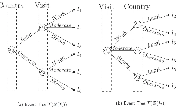
4.1 Event Trees yielded by the demographic variables Country and Visit 68 4.2 MAP CEG associated with the PC sequence . . . 97

4.3 Train booking MAP SCEG for demographic variable order I1 . . . 100

4.4 Train booking MAP SCEG for demographic variable order I2 . . . 101

(9)

5.2 NLP for a CEG with only one stage associated with Train . . . . 113

5.3 Examples of Dirichlet Local Prior and NLPs . . . 114

5.4 Train booking MAP SCEG for demographic variable order I1 (Copy)116

5.5 The event tree associated with the CHDS data set . . . 133

5.6 CEG Model for simulation studies with the CHDS data set . . . . 134

5.7 Average of the Number of Stages in the CHDS simulation study . 136

5.8 Total Situational Errors in the CHDS simulation study . . . 137

5.9 MAP CEGs for the CHDS data set according to different α¯-values 139

5.10 Five different MAP CEGs for the CHDS data set . . . 140

5.11 Generating BN Model for simulation studies about radicalisation . 144

6.1 DCEG depicted according to Barclay et al. (2015) . . . 153

6.2 Finite Event tree associated with the radicalisation process . . . . 155

6.3 The tree object ∆(_T)that symbolises a finite event tree . . . 156

6.4 The representation of an infinite Event Tree using tree objects . . 158

6.5 Infinite tree with time-invariant variables . . . 159

6.6 Two Staged Subtrees corresponding to the radicalisation process . 165

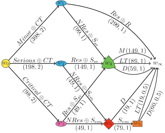
6.7 The 2T-DCEG associated with the radicalisation process . . . 171

7.1 A DCEG and a 2T-DCEG associated with the radicalisation process 175

7.2 A 2T-DCEG with time-invariant variables . . . 176

7.3 The state-transition diagram associated with a 2T-DCEG . . . . 179

7.4 The process of obtaining a CEG Ct, t≥2N −2, from a DCEG C 185

7.5 The CEG C2 associated with a 2T-DCEG . . . 191

7.6 Interrogating a 2T-DCEG . . . 195

(10)

7.8 A simple 2T-DCEG for the radicalisation process . . . 212

(11)

Acknowledgments

My thanks go first to professor Jim Q. Smith who has been an encouraging, friendly and zealous supervisor. His stimulating and insightful advice has inspired me to bring this work to fruition. His constant availability, patience and openness for discussions have played a key role in this thesis and represent his generosity and his work ethnic as regards his students and colleagues.

I wish to thank the 15-month and 24-month panel members, Dr. David Rossell, Prof. Jane Hutton and Prof. Simon French for their important feedback. In partic-ular, Dr. David Rossell provided valuable comments on non-local priors. I am also grateful to John Horwood and the CHDS research group for providing the CHDS data set and to Prof. James Henry and Dr. Geraldine Mcleod for allowing me to present the results associated with the process of booking a tourist train. Thank you, too, to all the members of the Statistics Department, especially the Admin-istrative staff, for constructing an astonishing and inspiring research environment.

I am very privileged to have had many important and encouraging teachers through-out my academic life, especially in the Brazilian Naval Academy and in the Federal University of Rio de Janeiro (UFRJ/COPPE). Special thanks to Professors Antonio Luiz Porto e Albuquerque, Bas´ılio de Bragan¸ca Pereira, H´elio dos Santos Migon and Mozart Menezes for their support in my pursuit of this doctorate.

I am also fortunate to have some friends to help and motivate me. In particular I would like to thank Braz Lamarca, Leonardo Antonio Monteiro Pessˆoa and Pier Giovanni Taranti for their forbearance during my PhD course.

(12)

Brazilian Navy and CNPq-Brazil. I directly rely on the institutional support from the Naval Secretariat of Science, Technology and Innovations (SecCTM) and the Naval System Analysis Center (CASNAV). I am especially thankful to Vice Ad-miral Bernardo José Pierantoni Gambôa, Rear AdAd-miral Cid Augusto Claro Junior, Captain Marco Eugênio Madeira Di Beneditto, Captain Lucia Artusi, Captain Ana Cláudia de Paula and Dr. Ivana Cardial de Miranda Pereira for believing in my work.

(13)

Declarations

I hereby declare that this work is based on my own research under the supervision of professor Jim Smith, except when stated otherwise. This thesis has not been submitted for examination at any another university. Some of this work has been published as follows: the material in Chapter 5 has been published in theBayesian Analysis under the title “A new family of Non-Local Priors for Chain Event Graph model selection” (Collazo and Smith, 2016). It is also available as CRiSM Working Paper 15-02. That paper was written with Jim Q. Smith but the text in Chapter 5 is entirely my own work.

I am one of the co-authors in a preliminary paper concerning the dynamic version of Chain Event Graphs. This paper has been published in the Eletronic Journal of Statitics under the title “The Dynamic Chain Event Graph” (Barclay et al., 2015). It resulted from a joint work with Lorna M. Barclay, Jim Q. Smith, Peter A. Twaites and Ann E. Nicholson. It is also available as CRiSM Working Paper14-04. A seminal DCEG paper based on Chapters 6 and 7 of this thesis is currently being revised for submission. This work is co-authored with Jim Q. Smith.

(14)

(15)

Abstract

The Chain Event Graph (CEG) is a type of tree-based graphical model that accom-modates all discrete Bayesian Networks as a particular subclass. It has already been successfully used to capture context-specific conditional independence structures of highly asymmetric processes in a way easily appreciated by domain experts. Being built from a tree, a CEG has a huge number of free parameters that makes the class extremely expressive but also very large. Exploring the enormous CEG model space then makes it necessary to design bespoke algorithms for this purpose. All Bayesian algorithms for CEG model selection in the literature are based on the Dirichlet characterisation of a family of CEGs spanned by a single event tree. Here I generalise this framework for a CEG model space spanned by a collection of different event trees. A new concept called hyper-stage is also introduced and provides us with a framework to design more efficient algorithms.

These improvements are nevertheless insufficient to scale up the model search for more challenging applications. In other contexts, recent analyses of Bayes Factor model selection using conjugate priors have suggested that the use of such prior settings tends to choose models that are not sufficiently parsimonious. To sidestep this phenomenon, non-local priors (NLPs) have been successfully developed. These priors enable the fast identification of the simpler model when it really does drive the data generation process. In this thesis, I define three new families of NLPs designed to be applied specifically to discrete processes defined through trees. In doing this, I develop a framework for a CEG model search which appears to be both robust and computationally efficient.

(16)

Abbreviations

2T-DBN Two Time-Slice Dynamic Bayesian Network

2T-DCEG Two Time-Slice Dynamic Chain Event Graph Network AHC Agglomerative Hierarchical Clustering

BF Bayes Factor BN Bayesian Network CEG Chain Event Graph

CHDS Christchurch Health and Development Study DAG Directed Acyclic Graph

DBN Dynamic Bayesian Network DCEG Dynamic Chain Event Graph fp-NLP Full Product Non-Local Prior LP Local Prior

lpBF Logarithm of Posterior Bayes Factor MAP Maximum A Posteriori

NLP Non-Local Prior

NT-DBN N Time-Slice Dynamic Bayesian Network

NT-DCEG N Time-Slice Dynamic Chain Event Graph

NT-SDCEG N Time-Slice Stratified Dynamic Chain Event Graph OAHC Optimise Agglomerative Hierarchical Clustering pBF Posterior Bayes Factor

PC Point of Contact

(17)

(18)

Chapter 1

Introduction

1.1 Motivation

Graphical models are useful tools that facilitate the interaction among scientists of different areas, and between these and decision makers. They provide a visual framework focusing on the structural relations that characterize processes. This interface is particularly attractive since its essence can be appreciated even by laypeople with little mathematical training. The Bayesian network (BN) (Pearl, 1988, Neapolitan, 2004, Cowell et al., 2007, Korb and Nicholson, 2011, Smith, 2010) is the most widely used type of graphical model in the statistical domain. It has been applied in diverse areas such as: management, business, environmen-tal studies, military applications, computational engineering, biology, medicine, genetics, pedigree analyses and many others.

(19)

de-pict context-specific conditional independences (Spiegelhalter and Lauritzen, 1990, Boutilier et al., 1996), i.e. where conditional independences hold only for certain values of the conditioning probability vector.

To build classes of models that can accommodate such assumptions, various non-graphical methods have now been suggested and appended to the BN framework, including context-specific BNs (Boutilier et al., 1996, Poole and Zhang, 2003, McAllester et al., 2008) and object-oriented BNs (Koller and Pfeffer, 1997, Bangsø and Wuillemin, 2000). A graphical limitation of BNs is illustrated in Example 1. This describes a very simple version of the process associated with the refugee crisis in the Mediterranean Sea.

Example1 (Refugee Crisis). In the European refugee crisis, thousands of migrants lost their lives in the Mediterranean Sea trying to travel from North Africa to Southern European using flimsy boats. Suppose that we would like to model the

chance (variable C) of a migrant arriving alive in Europe (y- alive, n- dead) as

a function of the roughness of the sea (variable S). The variable S measures the mean wave height of the one third highest waves according to five categories:

a-less than 0.1m; b- between 0.1 and 1.25m; c- between 1.25m and 4m; d- between 4m and 6m; and e- greater than 6m.

Figure 1.1: The BN model corresponding to the chance (variable C) of a migrant arriving

alive in Europe as a function of the roughness of the Mediterranean sea (variable S).

Assume that the probability of success decreases monotonically as the wave height

increases and that there is no difference between categories a and b. Then Figure 1.1 shows the BN that represents this process. Suppose its hypothetical conditional

Observe that without adding dummy random variables we are not able to express

(20)

success is indeed zero for category e.

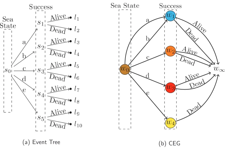
An alternative class of graphs which is able to at least depict structural asymmetries directly is an event tree; see Shafer (1996). By embellishing this structure with colours based on a probabilistic measure we obtain a probabilistic tree that provides the basis of a graphical framework called a Chain Event Graph (CEG) (Smith and Anderson, 2008, Thwaites et al., 2008, Smith, 2010). For further discussion, see Example 1 (cont.) below.

Example 1 (Refugee Crisis - cont.). The event tree in Figure 1.2a depicts the

multiple ways that the migration process can unfold for each refugee. Note that at this point domain experts do not need to consider variables or the conditional

independence relationships between them. The tree supports a modelling repre-sentation that allows them to focus instead on different qualitative descriptions of

the process.

[image:20.595.128.492.422.668.2]

(a) Event Tree _{(b) CEG}

Figure 1.2: The Event Tree and CEG model corresponding to the chance of a migrant

arriving alive in Europe as a function of the roughness of the Mediterranean sea.

(21)

the CEG that the conditional probability of success is identical given sea state

a or b. The probability zero of success associated with a sea state category e is directed incorporated into the CEG model by omitting its corresponding edge.

These graphical properties play an important role in more complex processes and,

particularly, in many practical dynamic scenarios where the probability conditional tables tend to contain more structural zeros.

The class of CEG models is closely related to the probabilistic decision graphs (Bozga and Maler, 1999, Jaeger, 2004, Jaeger et al., 2006) and encompasses the entire discrete BN class (Smith and Anderson, 2008). It also provides a useful framework for learning under complete sampling (Freeman and Smith, 2011a) model selection (Freeman and Smith, 2011a, Barclay et al., 2013) and causal analyses (Thwaites et al., 2010, Cowell and Smith, 2013). In addition to this it also supports efficient propagation of new information (Thwaites et al., 2008, Thwaites and Smith, 2006b) and studies with missing data (Barclay et al., 2014).

A probabilistic tree typically has a huge number of free parameters. This richness of models makes the class of CEGs extremely expressive, particularly when the underlying tree is asymmetric (French and Insua, 2010). However the space of models is consequently immense even for problems described by a fairly moderate number of random variables. In order to find useful CEG models it is therefore necessary to design bespoke model search algorithms. This can require us to make use of various heuristic methods (Silander and Leong, 2013, Cowell and Smith, 2014). Dirichlet conjugate learning for CEGs (Freeman and Smith, 2011a) provides us with a natural and efficient framework to do this because the score functions of different models can be expressed analytically and in closed form.

(22)

of our model space, any method which biases the model search to simpler models can turn out to be extremely useful.

Another contentious issue common with all Bayesian search methods is that the values of the hyper-parameters of standard Dirichlet priors need to be set to ini-tialise the model search. Although, at least from a subjectivist perspective, this is not a problem in terms of Bayesian estimation, it is a problem when addressing model selection, since it would be impossible₋ common with all Bayesian search methods − in practice to reflect on the massive number of appropriate values of possible explanatory model hyperparameter vectors individually.

One common way to attempt to circumvent these issues is to adopt a vague prior. However, it has been known for some time that this reduces the robustness of the model selection by making the result dependent on the parameter that sets the vagueness of beliefs a priori (Rao and Wu, 2001, Berger and Pericchi, 2001, Pericchi, 2005). This and related instabilities have also been reported for a graphical model in the BN context (Steck, 2008, Silander et al., 2007, Steck and Jaakkola, 2002). Such instabilities can also occur when searching the class of CEG models if care is not taken especially when using standard conjugate local priors BF model selection (Silander and Leong, 2013, Collazo and Smith, 2016). In this thesis, both to obtain parsimonious models and to guarantee the stability of the model selection I will develop new families of prior distributions specifically designed for discrete processes supported by trees.

(23)

is designed for a different purpose: to describe how a single cohort of units who arrive in the system simultaneously might evolve over successive time points under the hypothesis of time-homogeneity after some timeT.

Of course, the Dynamic Bayesian Network (DBN) provides a well-established graphical framework for discrete processes that develop over time: see Dabrowski and de Villiers (2015), Rubio et al. (2014), Marini et al. (2015), Li et al. (2014), Sun and Sun (2015), Khakzad (2015). A DBN corresponds to an extension of a BN for modelling and reasoning within dynamic systems whose progress is recorded over a time sequence. However despite their flexibility, because they are based on a Directed Acyclic Graph (DAG) a DBN has the same drawbacks that a BN has.

So, it is clearly time to develop a Dynamic Chain Event Graph (DCEG) to model longitudinal data. Tree-based graphical models provide a powerful graphical frame-work through which sequences of events that happen over time can be directly accommodated. For example, each possible time sequence can be described by a particular path in the event tree. This enables domain experts to express their beliefs about dynamic process in terms of events rather than random variables. It also provides graphical support for embodying logical constraints and context-specific statements that may change over time and managing sparse conditional probability tables without requiring additional dummy or degenerate variables.

In Barclay et al. (2015) a very general dynamic class of CEG models was de-fined. Despite this generality the methods in that paper did not provide a formal framework for systematically constructing a DCEG and reading the conditional independences it entailed. Furthermore, these authors admitted that model se-lection over this immense class of models was extremely challenging. This arose because the DCEG model space could be huge even for quite small problems. To develop bespoke algorithms to search this massive model space for explanatory and causal mechanisms in moderately sized problems therefore requires us first to define useful and pertinent subclasses of DCEGs to search over.

(24)

1. Can we construct a family of prior distributions that ensure parsimony and stability of CEG model selection to the setting of hyper-parameters, partic-ularly when greedy model search algorithms are used?

2. How can we formally define a general class of DCEGs in discrete time? How can we systematically construct it?

3. Is there a useful subclass of DCEGs? How can we interpret it? What are their properties?

Below I will outline the thesis plan for approaching these research questions.

1.2 Thesis Outline

In Chapter 2, I will briefly review the concepts that support the construction of graphical models. I next focus on discrete BN models since this model class is one of the most well-established graphical frameworks in the scientific community. I will present their graphical semantics and the Bayesian methods for learning an appropriate graph from complete data using a characterisation of Dirichlet priors. Finally, I will introduce the DBNs and highlight some important limitations of BNs and DBNs through specific examples.

Of course, there are several methods for learning graphical models and making inferences within them. Perhaps the two most principled frameworks adopt either a relative frequency approach or a Bayesian approach to probability, see e.g. the discussion in Neapolitan (2004) and Cowell et al. (2007). Throughout this thesis I have chosen the latter for three main reasons. First, I am inclined to use the Bayesian methodology for various technical reasons outlined in Howson and Ur-bach (1994), Krause and Clark (1994), Lindley (1994) and O’Hagan and Forster (2004).

(25)

running the models at certain settings within the examples used in this thesis I find that many cells are empty or sparse. Again through using a graphical model this gives rise to no technical issues other than the fact that the prior drives the inference and comparisons can be performed homogeneously through the model space.

Chapter 3 will be dedicated to the CEG framework. I will explain how to construct a CEG model and how to use it to explore the conditional independences that may be present in the data. I will then discuss the conjugate Bayesian learning based on Dirichlet priors (Freeman and Smith, 2011a) and the advantages of propagating evidence using a CEG model. At this point I will propose a modified and more efficient version of the propagation algorithm developed by Thwaites and Smith (2006b). All these concepts will be further illustrated using a new real-world process of booking a tourist train and an extended version of the example on kidney and liver disorders first analysed by Thwaites and Smith (2006b).

In Chapter 4 I will discuss the CEG model search algorithms developed in the literature. I will first review Bayes Factor model selection and a formal Dirichlet characterisation of CEG models when the graphs in the CEG model space share the same event tree. I will then propose an extension of this framework for a CEG space model which is spanned by a collection of event trees. In order to do this I assume two further conditions that are often adopted for BN model selection. I will also review a useful family of CEG models called Stratified CEGs (SCEGs) (Cowell and Smith, 2014). The SCEG models constitute an important CEG class because it contains all discrete BNs and context-specific BNs (Boutilier et al., 1996, Poole and Zhang, 2003, McAllester et al., 2008) as a special case. The SCEG subclass enables us to explore many plausible collections of explanatory hypotheses even though it is smaller than the full CEG class.

(26)

greedy model search algorithm developed by Freeman and Smith (2011a) and analyse some possible ways of improving it. I will then propose a modified version of this algorithm that is able to search the CEG model space more efficiently. Through this development a new concept called hyper-stages is appended to the CEG framework. As I will show, a hyper-stage structure enables us not only to design a more efficient algorithm but also to embellish the qualitative description of our models by accommodating domain hypotheses within the model search.

I will then review a dynamic programming algorithm (Bellman, 1957) for SCEG models as presented in Cowell and Smith (2014). Although this method guarantees that the MAP CEG will be found, those authors recognised that it can easily become unable to explore CEG model spaces of fairly moderate sizes and that the development of reliable approximative algorithms is needed. I will discuss these challenges and propose some strategies for minimising them. Finally, I will revisit the booking train example and explore the space of possible explanatory hypotheses for this process using the dynamic programming model search algorithm. The results have already been reported in Collazo et al. (2016).

The next three chapters constitute the most original and relevant methodologi-cal contributions of this thesis. In Chapter 5, I will review the model selection methods based on non-local priors (NLPs) (Johnson and Rossell, 2010, Consonni et al., 2013, Consonni and La Rocca, 2011, Johnson and Rossell, 2012, Altomare et al., 2013, Rossell and Telesca, 2015). Embodying a separation measure between nested models within their constructions, these priors automatically penalise com-plex models although these are still consistent in the Bayesian framework. For this reason, an NLP is more able to retrieve a parsimonious model than standard priors such as those based on conjugate learning when the simpler model is truly the source of the data generation process.

(27)

occur when standard Dirchlet priors and product NLPs are used in conjuction with some greedy model search algorithm. I will argue that pm-NLPs provide a promising and simple way to render the model search more robust and to identify parsimonious CEG models in high-dimensional settings where conditional depen-dence structures tend to be sparse. I will then proceed to develop a CEG model search framework that will allow us to use pm-NLPs in conjunction with my mod-ified greedy model search algorithm introduced in the previous Chapter.

To explore empirically the good properties of pm-NLPs, I will conduct extensive computational experiments for CEG model searches using two real-world examples and an R package for CEGs that I have collaboratively developed (Collazo and Taranti, 2016). First I will revisit a well-studied data set on childhood hospitalisa-tion (Fergusson et al., 1981, 1984, 1986, Barclay et al., 2013, Cowell and Smith, 2014). My method will be shown to provide us with more robust results to the setting of hyper-parameters than standard Dirchlet priors. It will also be able to give new insights into the dynamic between the risk of a child being hospitalised and the socio-economic factors that characterise his family background.

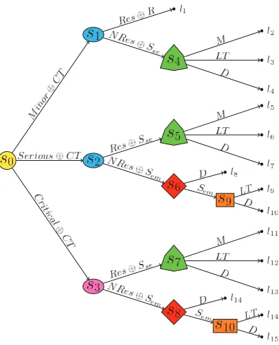
To illustrate how these selection methods scale up to large problems I will look at the process of radicalisation of inmates in British prisons. This topic has become a high priority for policymakers and an issue of lively public debate since experts have recognised the fundamental role that prisons can have as a hot house for radicalisation. Indeed, some empirical evidence indicates that extremist ideologists can be highly compelling amongst certain classes of inmates.

(28)

effi-cient algorithms that combine prior domain information and data. In this thesis, the explanatory variables can capture the ethnological and criminal background of prisoners as well as their prison networks. For all these reasons this application was actually beyond the scope of the search algorithms discussed in Chapter 4. Note that a summary of Chapter 5 has already been published in Collazo and Smith (2016).

In Chapters 6 and 7, I will define a new discrete multivariate dynamic model, the

Dynamic Chain Event Graph (DCEG), that is a natural counterpart of a Chain Event Graph. I contributed to the first paper that introduced these processes (Barclay et al., 2015). To advance the foundation of this new model class in discrete time here I have focused on the following three objectives:

1. To develop a practical methodology to guide the construction of effective DCEGs in practice using new classes of DCEGs which can coherently dis-tribute domain judgements as symmetries across different teams of experts. 2. To introduce new graphical semantics to express context-specific conditional independence structures often only implicit in the composed domain beliefs elicited during the knowledge engineering process.

3. To develop formal methods to identify the random processes intrinsic to an elicited probabilistic structure, and also to explore the implicit conditional independence structures between these processes.

Throughout these Chapters all concepts will be illustrated and further discussed using an example that models dynamically a simple radicalisation process of a prison population. This development has already been reported in Collazo and Smith (2016) and submitted for review.

(29)

graphical modellers to incorporate time-invariant variables in a DCEG model and to split the modelling task between different domain expert teams. This ensures the consistency of the composite model. In Section 6.2, I will introduce a formal framework to embed a probabilistic map on an infinite tree and discuss some topological concepts on probabilistic trees. In the concluding Section 6.3 I will formally define a DCEG and give a general representation of a finite DCEG in terms of a particular graphical periodicity and time-homogeneity.

In Chapter 7, I will introduce a new model class I have devised called N Time-Slice Dynamic Chain Event Graph (NT-DCEG). Such a DCEG class will have the potential for modelling several different processes in real-world applications. It will also enable us to develop bespoke algorithms to search the massive DCEG model space for useful explanatory models and causal mechanisms.

A formal link between a Markov state-transition diagram and an NT-DCEG will also be constructed as well as some links between DCEGs and DBNs. In particular I will prove that a Two Time-Slice Dynamic Bayesian Network (2T-DBN) can always be expressed as a 2T-DCEG. I will then explain how a particular set of CEGs can be used to derive a DCEG model. The connection between a DCEG and a corresponding set of CEGs will be then analysed.

(30)

Geweke (1984), Eichler (2007) and Eichler and Didelez (2010).

(31)

Chapter 2

Graphical Models

I start this chapter reviewing graphical models and graph theory. I then proceed to discuss various statistical properties corresponding to one of the most popular graphical models, the Bayesian Network (BN), and its dynamic counterpart, the Dynamic BN. I finish by outlining some of the limitations of BN models.

2.1 An overview of Graphical Models

In order to use graphical models, it is necessary first to define the semantics. This connects the graphical symbols with the theoretical or applied domain. In other words, the semantic lexis establishes the function, scope and use of each symbol. Therefore, the potential and limits of any graphical model are given by this initial semantic definition.

Graphical models become statistical models when their semantics relates the topol-ogy of the graph to the probability measure associated with a class of probability models; a condition which is satisfied for all graphs considered here. I here restrict myself to discrete model graphs. That is, I only consider problems whose observed random variables are discrete, although the parameters defining these variables can be (and usually are) continuous quantities.

I also restrict my focus to graphical models whose topologies include a graph

(32)

setV depicts the main elements of a domain as stated by the qualitative modelling; for example, variables, situations, decisions and so on. The set E represents the relationship among the previous elements according to the semantic lexis. In general, this set introduces the probabilistic map over the model. The topology may have other elements such as colours and different shapes of vertices, but the graph provides the framework which is then populated with for these additional elements.

In a broad sense, the use of a graphical model in a specific domain relies on the following steps: domain modelling; learning of the model; and inference and manipulation (Cowell et al., 2007). The first step corresponds to the qualitative modelling and requires us to answer the following questions: i) Which objects in the domain constitute the vertices?; and ii) How do these elements relate to each other, i.e. which edges constitute the set E? This early step typically demands a deep knowledge of the field and, consequently, the active participation of the domain experts. Within this phase, the pictorial representation of the model helps the interaction between the experts and the statistical specialists, implicitly embedding the problem within the statistical representation.

In the second phase, the statistician needs to populate the model with probabilistic distributions. This quantitative elicitation can be obtained by adopting a subjective or an objective-based modelling approach. In the first case the analyst uses some formal framework to map the experts’ prior beliefs into subjective probabilities (Wright and Ayton, 1994) associated with the random variables defined in the qualitative model. Here, the graphical model is an important and valuable tool to help experts elicit their knowledge a priori. It helps to prevent experts from losing focus in a welter of tangential technicalities or freezing when they address high levels of complexity. However, those probability distributions can also be defined using exclusively a data set. This corresponds to adopt an objective approach.

(33)

because it is rather difficult to obtain sufficient reliable data in order to conduct the data-driven learning process for the whole model. Another reason is that embedding domain information allows the analyst to obtain models that are more appealing for decision makers and domain experts. In many settings this approach also helps to reduce the modelling complexities and to keep the computational costs under control.

Remember that data can drive not only the definition of probabilistic distributions in the second phase but also the specification of the set of edges that constitute the qualitative structure of the model: answer the second question in the first phase. The intrinsic properties of the graph are used to carry out model selection and model learning, optimizing the performance of the chosen model or pool of models. In a strict objective approach the analyst is almost the only actor responsible for the learning process and the interaction with the domain expert rarely happens.

Finally, the statisticians will analyse the obtained results and present the initial feedback to the domain experts. Here, the graph is a helpful resource to stimu-late the experts’ interaction and to underpin the subsequent rounds of analysis, inference and manipulation. It enables the domain experts to consider the results in a very intuitive and direct way, thus helping the statistician to translate very advanced technical concepts into an objective and common language.

2.2 Introduction to Graph Theory

In this section I review some concepts of graph theory that will be important for the development of this thesis. For further details, see e.g. Netto (2006), Diestel (2006) and Cowell et al. (2007).

Definition 1 (Graph). Agraph Gis a pair G= (V, E), whereV =_{v1, . . . , vN}

is a set of vertices and E is a set of edges (vi, vj)∈V ×V between the vertices

(34)

Definition 2 (Subgraph). A graphGs = (Vs, Es) is a subgraph of G= (V, E) if

Vs ⊆V and Es⊆E.

Definition 3 (Undirected and Directed Graphs). An undirected graph is a graph

˜

G= ( ˜V ,E)˜ whose edges have no directionality and are calledundirected edges. In this case each undirected edge(vi, vj)∈E˜ is depicted as a line betweenvi and vj.

In contrast, adirected graph G= (V, E) is a graph whose every edge (vi, vj)has

an orientation. A directed edge (vi, vj)∈E is graphically represented as a arrow

from vi to vj. We can obtain an undirected version G˜ = ( ˜V ,E)˜ of a directed

graph G = (V, E) by removing the directionality of every edge in G. Explicitly, we then haveV˜ =V and E˜ =_{(vi, vj),(vj, vi); (vi, vj) or (vj, vi)∈E}.

Definition 4 (Labelled Graph). A labelled graph G is a graph G = (V, E, RV),

where RV = {(v, lv);v ∈ V} is the set of labels lv over each vertex in V,

E =_{(vi, vj, le); (vi, vj)∈V ×V} is the set of labelled edges such that the triad

(vi, vj, le)represents an edge (vi, vj) with label le.

Definition 5 (Multi-Graph). A graph G = (V, E) is said to be a multi-graph if there can be two or more edges(vi, vj)between any two vertices vi and vj in V,

otherwise the graph is called simple.

Definition 6 (Parent and Child). In a directed graphG= (V, E)a vertexv ∈V

is a parent (or a child) of a vertex vn ∈ V if (v, vn) ∈ E (or (vn, v) ∈ E). Let

pa(vn) = {v ∈ V; (v, vn) ∈ E} denote the parent set of a vertex vn ∈ V and

ch(vn) = {v ∈V; (vn, v)∈E} denote the children of a vertex vn∈V.

Definition 7 (Adjacent Vertices). Two vertices vi and vj of a graph G are said

to be adjacent if there is at least one edge between them.

Definition 8(Walk, Path and Trail). In a graphG= (V, E)awalk of lengthLis a sequence of vertices(vi0, . . . , viL)such that every edge(vik, vik+1),k= 0, . . . , L−1,

pertains to E. A walk that no two vertices are repeat is called a path. A trail of length L is a sequence of distinct vertices (vi0, . . . , viL) such that at least one of

(35)

trail(vi0, . . . , viL)of a directed graph G= (V, E) a vertexvk, k = 0, . . . , L−1is

called acollider vertex if the edges (vik−1, vik) and (vik+1, vik)pertain to E. Definition 9 (Descendent and Ancestor vertices). Take a DAG D = (V, E). A vertexv is adescendent of a vertex va inDif there exists ava-to-v path but there

is not a v-to-va path. Conversely, v is an ancestor of a vertex va in D if there

exists a v-to-va path but there is not a va-to-v path. A subset V∗ ⊆ V is called

an ancestral set if for everyv ∈V∗ we have that pa(v)⊆V∗. Let An(V∗) be the

smallest ancestral set that contains V∗.

Definition 10 (Connected Graph). A graphG = (V, E) is said to be connected

if there is a trail between every pair of its vertices. A component of a graphG is a maximal connected subgraph of G.

Definition 11(Cycle). In a graphG= (V, E)a cycleof lengthLis a sequence of vertices (vi0, . . . , viL) such that(vi0, . . . , viL−1) is a path and such that vi0 =viL

and (viL−1, viL)∈E.

Definition 12 (Directed Acyclic Graph). A directed acyclic graph (DAG) is a directed graph without cycles. A DAG D= (V, E)yields an ordering

O(V) = (vi1, . . . , viN)

over the vertex setV=_{v1, . . . , vN}such that for any two verticesvia andvib, b > a,

there does not exist an edge(vib, via)inE. If for every vertexvin,n= 1, . . . , N−1,

the edge(vin, vij),j =n+1, . . . , N, is inE, then the DAG is said to be complete. Definition 13 (Tree). A tree _T = (V, E) is a connected simple graph whose undirected version has no cycles. Any vertex in V can be designated as the root vertex v0 and the tree is said to be rooted. A leaf vertex is a non-root vertex of

a tree that has only one adjacent vertex. In a rooted tree a vertex v is said to be at a level ℓd if the v0-to-v path has length d. In this thesis all trees are assumed

to be directed and rooted. This implies that the root vertex v0 has no parents

(36)

Definition 14 (Star). A tree that has at maximum one vertex connected to two or more other vertices is called a star.

Definition 15 (Forest). A forest is a graph whose every component is a tree.

2.3 Introduction to Bayesian Networks

A BN model is a pair B = (D,P₎_{, where} _D _{= (V, E)} _{is a DAG and} P _{is a}

probabilistic measure. Recall that in a DAG D = (V, E), the set of vertices is given by a well-ordered set V = {v1, . . . , vn}, where each vertex vi represents a

variable_Zi, and the edge setEcontains a collection of directed edge(vi, vj), i < j.

The edges in E enable analysts to describe whether a particular variable provides any relevant probabilistic statement to explain another variable given a set of contextual information.

In a BN, the encoding of probabilistic hypotheses is possible due to the con-cept of conditional independence. For example, take three discrete random vari-ables Z1, Z2 and Z3 whose set of categories are, respectively, Z1 = {1, . . . , L1},

Z2 ={1, . . . , L2} and Z3 = {1, . . . , L3}. If a domain analyst believes that

col-lecting information on the value of Z2 once the value of Z3 is known brings no

further improvement to explain variableZ1, thenZ2 is not probabilistically relevant

to variable Z1 given the value of Z3. In this case we say that Z1 is conditionally

independent from Z2 given Z3. This implies that for every triad (z1, z2, z3) in

Z1×Z2×Z3, we have that p(Z1 =z1|Z2 =z2, Z3 =z3) =p(Z1 =z1|Z3 =z3).

This idea directly generalises for random vectors and continuous probabilistic mea-sures as formally stated in Definition 16.

Definition 16(Conditional Independence). Take three random vectorsX,Y and

Z in a probability space (Ω,A_,P₎_{. We say that} _X _is _{conditionally independent}

of Y givenZ underP_{, and write}_X _⊥_⊥_Y_|_Z_{, if and only if for every set} _A_∈A

(37)

alone, i.e.

X _⊥_⊥Y_|Z _⇐⇒ P(X _∈A_|Y,Z) =P(X _∈A_|Z), (2.1)

whenever p(y,z) is strictly positive.

LetZ(m) ₌_{Z

1, . . . ,Zm} denote the firstmvariables of a set of ordered random

variablesZ ₌_{Z₁_{, . . . ,}_Z_N_}_{in a probability space}_(Ω,A_,P₎_{. Also let}_pa(Z_j_{) =} {Zi ∈ Z(j−1);vk ∈ pa(vj)} be the parent set of Zj with respect to D. We can

now introduce a useful Markov property that enables us to relate a probability measure to a graphical topology.

Definition 17(Ordered Markov Property (OMP)). Take a set of ordered random variables Z _{in a probability space} _(Ω,A_,P₎ _{and a DAG} _D_{. The probability}

measure P _{satisfies the} _{ordered Markov property} _{relative to} _D _{if for every pair}

of non-adjacent vertices vi and vj in V, i < j, a variable Zj is conditionally

independent of a variable Zi, i < j, given its parent set pa(Zj).

Now we can use the OMP to formally define a BN model.

Definition 18(Bayesian Network). ABayesian Network (BN) is a graphical model constituted by a set of random variables Z _{in a probability space}_(Ω,A_,P₎_and

by a DAG D such that the probability measure P _{satisfies the ordered Markov}

property relative toD.

Example 2 below presents a naive BN model to describe the radicalisation process of inmates in a prison system.

Example 2 (Radicalisation Process). A model of a male prisoner’s radicalisation within prisons uses as explanatory variables his social networks and how the

popu-lation is affected by prison transfers (Hannah et al., 2008, Neumann, 2010, Silke, 2011). The physical movements and social interactions of prisoners are constantly

being monitored and recorded. Here the radicalisation process is summarised by

(38)

take one of the following three levels: s- sporadic, f- frequent, i- intense. These

levels measure the frequency that a “standard” prisoner is able to socially interact with other prisoners who are identified as potential recruiters to radicalisation. A

binary variable T records whether an inmate remain in the prison (n) or is

trans-ferred (t) to another prison.

Figure 2.1: The BN associated with Example 2

Assume that the variable Transfer T is independent of the variable Network N given the variable Radicalisation R. Consider the hypothesis that all those prisoners

who have not adopted radicalisation are equally likely to be transferred. Figure 2.1

depicts a possible BN to represent this process.

Larger collections of conditional independence structures than those described by the OMP can be read from a BN model using the following properties satisfied by the ternary conditional independence relation (Dawid, 1979, Spohn, 1980):

Symmetry X _⊥_⊥Y_|Z _⇒Y _⊥_⊥X_|Z

Decomposition X _⊥_⊥(Y,W)_|Z _⇒X _⊥_⊥Y_|Z and X _⊥_⊥W_|Z

Weak Union X ⊥⊥(Y,W)|Z ⇒X ⊥⊥Y|(Z,W)

Contraction X _⊥_⊥Y_|Z and X _⊥_⊥W_|(Y,Z)⇒X _⊥_⊥(Y,W)|Z

These four properties constitute the semi-graphoid axioms. These allow analysts to explore the relevance of information using a graphical topology initially elicited (Pearl and Paz, 1987). If the probability measure P _{is strictly positive then the}

fifth properties given below also holds and we have a graphoid. For an intuitive interpretation of the graphoid axioms see Pearl (2009).

Intersection X _⊥_⊥Y_|Z,W and X _⊥_⊥W_|(Y,Z)_⇒X _⊥_⊥(Y,W)_|Z

(39)

Verma and Pearl (1990) and Geiger and Pearl (1990). To review this result, take two vertices va and vb of a DAG D = (V, E) and any subset VS ⊂ V\{va, vb}.

A trail τ between va and vb is said to be blocked by VS in D if there is a vertex

v _∈τ such that one of the conditions holds:

1. v pertains toVS and v is a non-collider vertex with respect to τ; or

2. v is a collider vertex inτ but v and all its descendants are not inVS.

If every trail betweenvaandvbis blocked thanvaandvb are said to bed-separated

by VS. It then follows that two disjoint subsets VA and VB are said to be

d-separated by a subset VS ⊂ V\(VA∪VB) if and only if every pair of vertices

(va, vb), such that va ∈Va and vb ∈VB, are d-separated by VS.

Theorem 1 (d-Separation Theorem,Pearl (1986, 1988)). Assume a BN model

B = (D,P₎_{, where} _D _{= (V, E)} _{and take any three disjoint subsets} _V_A_, _V_B _and VS of V. Let ZA, ZB and ZS be the set of random variables corresponding,

respectively, to VA,VB and VS. It then follows that

Z_A_⊥_⊥Z_B_|Z_S _⇐⇒ _V_S _d-separates _V_A _and _V_B_. _(2.2)

The property in Equation 2.2 is often called a global Markov property.

In Lauritzen et al. (1990) and Cowell et al. (2007), the d-separation theorem is rewritten using an undirected graphDM(A∪B∪S) = (VM, EM)corresponding to

a transformation of DAG D= (V, E) spanned by VA, VB and VS by the following

steps:

1. Take the graph Danc = (Vanc, Eanc), where Vanc =An(VA∪VB∪VS) in D

and Eanc ={(vi, vj)∈E;vi, vj ∈V}.

2. Construct the graphDM(A∪B∪S) = (VM, EM)fromDanc, whereVM =Vanc

and EM = ˜Eanc∪Emar. E˜anc is the set of undirected edges corresponding

toEanc, i.e,E˜anc ={(vi, vj); (vi, vj)∈Eanc}. Emar is the set of undirected

edges between any pair of vertices (vi, vj), i < j, in VM, such that in Danc

(40)

In an undirected graph G = (V, E) VS is said to separate VA and VB, where

VA∪VB∪VS are any three disjoints subsets of V, if every path between any pair

of vertices (va, vb), va ∈ Va and vb ∈ VB, passes through VS. The criterion of

d-separation as presented in Theorem 1 can then be restated as follows:

Z_A_⊥_⊥Z_B_|Z_S _⇐⇒ _V_S _separates _V_A _and _V_B _in D_M(A_∪B_∪S). (2.3) This alternative formulation is often more useful and appealing operationally.

Using the d-separation property domain experts can identify local conditional in-dependence structures that potentially characterise their processes. Therefore the qualitative aspects of a process can more deeply analysed and detailed and the probability distributions embedded within a model can be more precisely elicited and calibrated. The d-separation theorem also provides us with a solid criterion with which to manipulate and factorise complex graphical structures into local graphical components with simpler topologies. These local subgraphs constitute a key aspect that enables us to design and justify efficient inference and model selection algorithms: see e.g. Cowell et al. (2007), Korb and Nicholson (2011), Neapolitan (2004) and Smith (2010).

It is also shown that in a BN modelB= (D,P₎ _{the probability measure} P _over

the set of random variablesZ _{recursively factorizes as follows:}

p(Z =z_|D) = Y

Zi∈Z

p(Zi =zi|Zpa(Zi)=zpa(Zi)), (2.4)

where Z = (Z1, . . . , ZN)and Zpa(Zi) = (Zi1, . . . , Zik) are random vectors whose

every component is, respectively, a random variable in Z _and _pa(_Z_i₎_{. This also}

implies that in a BN modelB= (D,P₎_{every variable is conditionally independent}

of its non-descendent variables with respect to Dgiven its parent set. For further details see e.g. Cowell et al. (2007).

2.4 Introduction to Dynamic Bayesian Networks

(41)

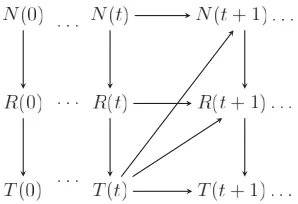
rela-tionship among variables that are observed at regular time intervals. So henceforth in this thesis we letZ_(t)_{be a set of random variables}Z_{observed at time-interval}_t

and whose total ordering is not necessarily identical over time.

Assume that a DAG D(T) = (V(T), E(T))) represents the conditional indepen-dence relationships between the components of Z_(T₎_{. Now define the set of}

temporal edges E†(T). These are edges from a vertex vi(t)∈ V(t), t < T, to a

vertex vj(T)∈V(T) and so represent relationships between variables in different

time-slices. Note that there might be a temporal edge (vi(t), vi(T)). This would

depict the dependence of a variable _Zi at time T on its value at any previous

timet,t < T. Inherinting the usual semantics of a BN, two non-adjacent vertices

vi(t) ∈ V(t) and vj(T) ∈ V(T), such that t ≤ T and, if t = T, i < j, then

imply that _Zj(T) is conditionally independent of a variable Zi(t) given its parent

set pa(Zj(T)), where pa(Zj(T))⊆ ∪Tk=0−1Z(k)∪Z(j−1)(T).

Therefore, a DBN model for the first T time-intervals consists of a probability measure P _{associated with the set of random variables} _∪T

t=0Z(t) and a DAG ¯

D(T) = ( ¯V(T),E(T¯ )), where V¯(T) =∪T

t=0V(t) and E(T¯ ) =∪Tt=0(E(t)∪E†(t)).

Without further assumptions, the specification of a DBN model is challenging since for each time-slicet a different DAGD(t)and its corresponding temporal edge set needs to be defined. So for practical reasons two additional conditions are often hypothesised. The first of these is to assume a Markov condition of order N₋1. This demands that the values of a variable at time t depend only on the values of variables at the lastN−1 previous and current intervals. The second common hypothesis is to assume that the process is time-homogeneous.

(42)

all subsequent intervals and its corresponding set of temporal edges E†(t) ≡E†.

When these two additional assumptions are adopted a DBN is called a N Time-Slice DBN (NT-DBN). A common choice in practice is to setN = 2, see e.g. Korb and Nicholson (2011), Neapolitan (2004), Pourret et al. (2008). This implies that the current value of a given variable may persist in the system at maximum one time-slice ahead. In this case, the state of the system at timet+ 1 is completely determined by the values of its variables at time t. This simplification provides satisfactory result particularly in systems that evolve slowly over time and if we are interested in filtering and forecasting over short-term time horizon.

Example 3 (Dynamic Radicalisation Process). Radicalisation has a psychosocial dynamic, which is naturally modelled as a process developing over time (Hannah

et al., 2008, Neumann, 2010, Silke, 2011, Christmann, 2012, Guittet et al., 2012, Schmid, 2013, Demetriou et al., 2014). Here suppose that the counts of this

process are recorded weekly and that the hypotheses in Example 2 are still valid for each time-slice. Being an isolated environment, a change in its underlying

mechanisms only happens rarely in the short to medium term: the very recent

events are the main psychosocial drivers of the prison population. In this scenario, it is plausible that the time-homogeneous and 1-Markov conditions might hold.

So, to define the temporal edges assume that all variables at time t+ 1 depend

only on their previous value and the value of the variable Transfer T at time t.

A prisoner with an extreme political or religious ideology typically constructs social

networks that are unlikely to moderate him and might well reinforce his current

beliefs. In this case, his social contacts reflect his personal vision of the world and his disengagement from militant extremism often requires personal incentives only

available after he leaves the prison. On the other hand, the conversion of a

non-radical prisoner to an extremist ideology can well be driven by his social contacts within the prison regardless of whether he is resilient or vulnerable. Under this

reasoning the social network might act on the prisoner’s belief system but not the other way around.

(43)

[image:43.595.234.383.106.208.2]

Figure 2.2: 2T-DBN associated with Example 3

that the type of psychological models described above are often called escalation

models (Wiktorowicz, 2004, Moghaddam, 2005, Silber and Bhatt, 2007, Gill, 2007, Precht, 2007, Audit Commission, 2008, McCauley and Moskalenko, 2008).

2.5 Learning the parameters of Bayesian Networks

In some contexts decision makers and domain experts can fully elicited the graphi-cal structure of a BN model and a graphigraphi-cal modeller needs only to use the data to learning it. However in many settings even the topology of the BN model needs to be learnt. For this purpose in a Bayesian framework a natural choice is to compare the posterior probability of each candidate BN model B. For example, take a BN model over a set of random variables Z ₌ _{Z₁_{, . . . ,}_Z_N_}_{, where each variable}

Zi, i = 1, . . . , N can assume Li values. Let Z = (Z1, . . . ,ZI) be a random

vector associated with I different units in the system, where Zi = (Zi1, . . . ,ZiN)

is a random vector that collects the values of each variable in Z _{for a unit} _i_,

i= 1, . . . , I. From the Bayes’ rule the posterior probability of a modelB is then given by

p(B_|z)∝p(z|B)p(B). (2.5)

(44)

distributions for each model in the BN model space can easily get intractable without further assumptions. In fact BN learning has been proved to be a NP-Hard problem in its general formulation (Cooper, 1990, Shimony, 1994).

Fortunately BN model selection is feasible by adopting some mild assumptions over both distributions p(B) and p(z|B). Here I will review how to learn a single discrete BN and its dynamic counterpart using a Bayesian approach. This is based on the characterisation of Dirichelet distributions (Heckerman et al., 1995), see also Heckerman and Geiger (1995), Geiger and Heckerman (1997) and Heckerman (1999, 2008). The elicitation of prior distributions over the model space and further details about Bayesian model selection will be reviewed in Chapter 3 when I introduce CEG model selection methods.

LetQ_n=_{qni;i= 1, . . . , Qn}denote the set of possible configurationsqniof values

that the parents of a variableZn∈Z can take, where Qn=Q_Z_j_∈_pa₍_Z_n₎Lj. From

equation 2.4 we can see that it is necessary to specify a conditional probability dis-tribution for eachqni,n= 1, . . . , N,i= 1, . . . , Qn. Remember that in a Bayesian

framework this can be done by putting a probability measure on each conditional probability qni itself. Thus let the set of random vectors Πn={πn1, . . . ,πnQn}, n = 1, . . . , N, denote a collection of random vectors πni = (πni1, . . . , πniLn), i = 1, . . . , Qn, such that πnij, j = 1, . . . , Ln, is the probability that a variable

Zn∈Z takes value k given that its parent set has configuration qni.

Now consider the following conditions:

Global Independence Random vectors associated with different variables are mutually independent.

Local Independence Random vectors associated with the same variable are mu-tually independent.

Parameter Modularity If a variable Zn ∈ Z has the same parent set in two

different BN models then the set of random vectorsΠ_n _{is the same for both}

models.

(45)

ex-pressed as independent and identically distributed.

Structural Possibility For any given variable order a BN model corresponding to the complete DAG has strictly positive probability, i.e. p(B)>0.

Likelihood (or Markov) Equivalence The prior distributions over the param-eter spaces of any two BN models that represent exactly the same set of conditional independence statements are identical.

Assuming the conditions above, Heckerman et al. (1995) showed that the prior and posterior distributions of each parameterπni∈Πn,n= 1, . . . , N andi= 1, . . . , Qn,

are inevitably Dirichlet distributions with hyper-parameters αni and αni +xni,

respectively. Herexni = (xni1, . . . , xniLn), where xnij,j = 1, . . . , Ln, denotes the

number of times that the variable Zn assumes value j in a sample z under the

configuration qni of its parent set. It then follows that the marginal likelihood of

a BN model is given by:

p(z_|B) =

N Y n=1 Qn Y i=1

Γ( ¯αni)

Γ( ¯αni+ ¯αni) Ln Y

j=1

Γ(αnij+xnij)

Γ(αnij)

, (2.6)

where Γ(·) is the gamma function, α¯ni = PL_j₌₁n αnij and x¯ni = PL_j₌₁n xnij.

Henceforward, for any n-dimensional vector γ_i = (γi1, . . . , γin) we convention

¯

γi =Pn_j₌₁γij.

A hyper-parameter αni, n= 1, . . . , N, i= 1, . . . , Qn, represents our prior belief

about each local structure, i.e, the conditional probability of a variableZn ∈ Zn

given a stateqni of its parent set. Recall that the prior expectation of a parameter

πni is given by

Eπni[πnij|αni] = αnij

¯ αni

. (2.7)

Thus a common way to set these hyper-parameters is to elicit the expected value of Eπni[πni|αni] for πni and then to set the strength α¯ni of our prior belief in

this elicited probability vector. Of course, it is still a problem to set these hyper-parameter vectors if there is a large set of candidate BN models. In this case the parameter modularity provides us with a simple and useful framework.

(46)

a full BN model, whereDC = (V, EC)is a complete DAG corresponding toZ. Set

a hyper-parameter αC _{for this full model and assume that for all} _n _{= 1, . . . , N}_,

i= 1, . . . , QC

n and j = 1, . . . , Ln

p(Zn =j|pa(Zn) =qniC,BC) =

αC nij

¯ αC

nij

. (2.8)

If there is a real number α such that for all n = 1, . . . , N, i = 1, . . . , QC n and

j = 1, . . . , Ln,

αC_nij =αp(Zn=j, pa(Zn) =qni|BC), (2.9)

then the BN BC is said to have an equivalent sample size equal to α. The

parameter modularity then guarantees that every BN modelB = (D,P₎ _over Z

has a hyper-parameter α given by

αnij =αp(Zn=j, pa(Zn|B) =qni|BC), (2.10)

for alln= 1, . . . , N,i= 1, . . . , Qn andj = 1, . . . , Ln. Note that in equation 2.10

the parent set pa(Zn|B) is defined with respect to B although the probability

measure corresponds to model BC.

Under the parameter modularity assumption specifying prior distributions for every BN in a model space therefore require us only to elicit the expected conditional probability tables of the full model and to define the equivalent sample size. When no prior domain information is available to guide us to set the hyper-parameters, a usual recommendation is to adopt a uniform distribution for each conditional prob-ability in Equation 2.8 and set the equivalent sample size equal to the maximum number of categories that a variable in Z _{can have, i.e.,} _α _{= max}_n_∈{₁_....,N_}_L_n_.

For detailed discussions on how to set the hyper-parameterα, see e.g. Heckerman et al. (1995), Heckerman (1999, 2008) and Neapolitan (2004).

(47)

a standard BN. Now note that in an NT-DBN we only have to learn N time-slices because of the Markov and time-homogeneity assumptions. So x records information ofN time-slices. It then follows thatx(t) =x∗(t),t= 0, . . . , N−2,

and x(N ₋1) =PT

t=N−1x∗(t).

2.6 Limitations of Bayesian Networks

A BN model provides us with a transparent graphical framework to define a process in terms of conditional independent local structures. This facilitates the identifi-cation of relevant structural components of the process, improves the accuracy of the elicited joint probability distributions and optimises the use of computational memory and time for inferences. Despite these strengths BNs are not always the appropriate graphical model to adopt because they represent a process using a preassigned collections of random vectors. In any setting where it is artificial to describe a process directly through a set of conditional probabilities between the given components of a multivariate process then its representation using a BN can be restrictive and often difficult to justify.

A BN model is particularly not recommended when a process has at least one of the following characteristics:

1. There are some context-specific conditional independence structures (Spiegel-halter and Lauritzen, 1990, Boutilier et al., 1996), see Definition 19 below. 2. The event space is a non-product space and so a process has highly

asym-metrical developments. This often happens when the state space of some variables changes or even does not exist depending on the value assumed by other variables in the probability space.

Definition 19 (Context-Specific Conditional Independence). Take three random vectorsX,Y andZ in a probability space(Ω,A_,P₎_{. We say that}_X _is context-specific conditionally independent of Y givenZ under P _{if and only if for some}

(48)

measurable with respect to a function ofZ =z alone, i.e.

X ⊥⊥Y|Z =z ⇐⇒ P(X ∈A|Y,Z =z) =P(X ∈A|Z =z), (2.11)

whenever p(y,z) is strictly positive. In this case, we write X _⊥_⊥Y_|Z =z.

In Example 2, without introducing new random variables the BN cannot represent graphically the context-specific hypothesis associated with the variable T given the variable R. This kind of asymmetric conditional independences can only be expressed inside the conditional probability tables of the BN or through some sup-plementary semantics. This fact is also true for the context-specific conditional independence statements in Example 3. Recall that the radicalisation model de-scribed here for the dynamic setting has two context-specific conditional indepen-dences in addition to that one specified in Example 2 : the variable RadicalisationR

at time t+ 1 is independent of the variable Network N at time t+ 1 given that the variable Radicalisation R assumes the value Adopting at previous time t; and the variable R at time t+ 1 is independent of its previous value at time t given that a prisoner did not adopt radicalisation at time t.

Also note that in the dynamic context when a prisoner is transferred the process terminates. However this kind of asymmetric development cannot be immediately read from the corresponding 2T-DBN.

Some extensions to the BN framework have been proposed to handle these issues. For example, a context-specific BN embellishes the BN/DBN models (Boutilier et al., 1996, Poole and Zhang, 2003, McAllester et al., 2008) using supplementary trees to represent the conditional probability tables that have context-specific in-formation. In this case each variable has its own tree. Alternatively, the standard BN can be reorganised in order to depict the context-specific independences using multiple vertices associated with a single variable.

Another proposal is to use Bayesian Multinets or Similarity Networks (Geiger and Heckerman, 1996). These adopt a hypothesis variable to encode the context-specific statements over a set of random variablesZ_{. For each value taken by the}

(49)

called local network. The collection of these local networks constitute a Bayesian Multinet or a Similarity Network.

The main difference between those models is that in a Bayesian Multinet all local networks need to depict all variables inZ _{whilst a Similarity Network depicts only}

the variables that relate to the hypothesis under consideration in a particular local network. To avoid losing information for not including all variables in every local network additional local networks are required and can then be identified through a similarity graph that models the set of hypotheses covered by the hypothesis variable.

An advantage of a Similarity Network is that the graphical modeller is not required to quantify the conditional probabilities between variables that are not covered by the hypotheses under analysis. However in both approaches, Bayesian Multinets and Similarity Networks, a process is described by a set of networks instead of a sin-gle graph. The natural consequence is that the modelling procedure becomes more complicated and the computational complexity to encode these models increases substantially compared to a standard BN. These problems only get worse when the hypothesis variable has to represent context-specific hypotheses associated with different states of the process.

(50)

model through objects tend not to be expressed graphically and so will remain hidden in conditional probability tables.

(51)

Chapter 3

A Chain Event Graph

In this Chapter I will demonstrate how the CEG framework can directly circumvent the drawbacks of BNs discussed in Chapter 2, namely modelling context-specific conditional independences and asymmetric event spaces. It will also become clear that a CEG model also retains the good properties of BNs, such as conjugate learning and efficient propagation of new information.