Variational methods for geometric statistical inference

(1)

University of Warwick institutional repository:

http://go.warwick.ac.uk/wrap

A Thesis Submitted for the Degree of PhD at the University of Warwick

http://go.warwick.ac.uk/wrap/74241

This thesis is made available online and is protected by original copyright.

Please scroll down to view the document itself.

(2)

Variational Methods For Geometric Statistical Inference

by

Matthew Thorpe

Thesis

Submitted to the University of Warwick

for the degree of

Doctor of Philosophy

Mathematics Institute

(3)

Acknowledgments

Firstly I would like to thank my supervisors Florian Theil, Adam Johansen and Neil Cade. I am very grateful for their help, spotting my mistakes and stimulating discussions. Without their guidance this thesis would not have been possible.

I would like to thank EPSRC and Selex ES Ltd. for funding my placement through a CASE studentship in the MASDOC program at the University of Warwick.

My thanks go to my friends Louise Mason, Tom Hull, Tom Wardell and Dan Wheble for their company over the last years.

I am grateful to everyone I have shared an office with (which for fear of missing someone I will not attempt to name) for answering both my sensible and naive questions. You have all helped me mathematically and distracted me when I needed it. In a related thanks I feel very lucky to have been part of MASDOC which has been an excellent community and is never short of people willing to drink wine on a Friday night.

Thanks also go to my ever increasing family and in particular my parents and grandpar-ents.

I am grateful to both examiners for their comments and feedback and also for both of them being very accommodating when coming to schedule the examination.

(6)

Declarations

This thesis contains original and collaborative research carried out during the author’s study in MASDOC (mathematics and statistics doctoral training centre) at the University of Warwick. The research was funded by an EPSRC CASE studentship with Selex ES Ltd. This thesis has been composed by myself and has not been submitted for any other degree or professional qualification. The work is my own, except where I have indicated to the contrary within the thesis. More specifically:

i) In Chapter 1, Section 1.1 is edited from a blog written with Neil Cade (Selex ES Ltd.) on the Smith Institute webpage [149].

ii) Chapter 2 is preliminary work in preparation for later chapters and contains no new results.

iii) Chapter 3 was joint work with Neil Cade, Adam Johansen (University of Warwick) and Flo-rian Theil (University of Warwick) and a version has been submitted for publication [154]. Corrections were made on the advise of two anonymous referees.

iv) Chapters 4 and 5 are joint work with Adam Johansen and versions have been submitted for publication [150, 151].

(7)

Abstract

Estimating multiple geometric shapes such as tracks or surfaces creates significant mathemati-cal challenges particularly in the presence of unknown data association. In particular, problems of this type have two major challenges. The first is typically the object of interest is infinite di-mensional whilst data is finite didi-mensional. As a result the inverse problem is ill-posed without regularization. The second is the data association makes the likelihood function highly oscilla-tory.

The focus of this thesis is on techniques to validate approaches to estimating problems in geometric statistical inference. We use convergence of the large data limit as an indicator of robustness of the methodology. One particular advantage of our approach is that we can prove convergence under modest conditions on the data generating process. This allows one to apply the theory where very little is known about the data. This indicates a robustness in applications to real world problems.

The results of this thesis therefore concern the asymptotics for a selection of statistical inference problems. We construct our estimates as the minimizer of an appropriate functional and look at what happens in the large data limit. In each case we will show our estimates con-verge to a minimizer of a limiting functional. In certain cases we also add rates of concon-vergence. The emphasis is on problems which contain a data association or classification compo-nent. More precisely we study a generalized version of thek-means method which is suitable for estimating multiple trajectories from unlabeled data which combines data association with spline smoothing. Another problem considered is a graphical approach to estimating the la-beling of data points. Our approach uses minimizers of the Ginzburg-Landau functional on a suitably defined graph.

(8)

Chapter 1

Introduction

“In theory, there is no difference between theory and practice. But in practice,

there is.”

- Yogi Berra

1.1 Motivation

Statistical estimators are used to extract information from data sets. Sometimes there may be some true value µ† which one hopes to recover in the large data limit, e.g. estimating the trajectory of a moving target from space-time measurements. Such a trajectory would form part of the data generating process. In other situation there may not be a true value of the parameter, e.g. deciding how to advertise products to a potential customer based on any available information, such as internet browsing history.

For the first type of problem it is natural to consider data{ξi= (ti, zi)}n_i₌₁of the form

zi =F(µ†, ei, ti) i= 1,2, . . . , n

whereeiis a random variable to account for noise,ziis an observation andtiis an input

param-eter. For example in the estimating trajectory problem one simple model is

zi =F(µ†, ei, ti) :=µ†(ti) +ei.

In many applications the functionF will have no inverse. Hence one cannot in general use the inverse ofF to reconstructµ†. One solution is to adopt a Bayesian-like approach.1 In general one constructs (the maximum-a-posterior) estimate µ(n) of µ† based on data {(ti, zi)}ni=1 by

solving

µ(n)= argmin

µ n

X

i=1

|zi−F(µ,0, ti)|2+λnR(µ) (1.1)

1_{Technically without assumptions such as Gaussian noise and prior and with}_λ

(9)

whereR is a regularization term and λn is some appropriate scaling. In a fully Bayesian

ap-proach one should chooseλn = λto be constant and then (under Gaussian assumptions) one

can interpret λR(µ) as the covariance of the prior. This is not always possible as the above minimization problem may become ill-posed, a fact well known in the Bayesian inverse com-munity [4] and in the spline fitting comcom-munity [46, 117]. In such cases one may be able take

λn → ∞and still showµ(n) → µ†. There is a very active community that work on results of

this type, see for example [4, 55, 72, 134, 139, 162], and references therein.

For the second class of problems there is noµ†so it does not make sense to look forFas before. One can see thatFallows one to compare estimates with the data and therefore in some sense encodes the data generating model. Therefore withoutF one has to produce estimates without reference to any such model. As an example let us consider thek-means method which will also be the subject of Chapter 3 and Chapter 4. Given a data set{zi}ni=1 ⊂ Rκ it is the

objective of the k-means method to partition the data intokclusters. This is done by minimizing the functional

fn(µ) = n

X

i=1

min

j=1,...,k|zi−µj|.

Minimizersµ(n)= (µ(₁n), . . . , µ_k(n))∈Rk×κoffnare called cluster centers and the partitioning

is defined by associating each data point to the closest center. One can see thatfn does not

depend on the data generating model.

The problems we consider in this thesis involve estimators which do not directly use the data generating process (like the k-means method) and may also be ill-posed, requiring regularization as we saw at the start of this section. For example Chapter 3 and Chapter 4 use thek-means method where cluster centers are trajectories and data is space-time observations

{ξi = (ti, zi)}ni=1. One can write the estimator as a minimizer offnwhere

fn(µ) =

1

n

X

i=1

min

j=1,...,k|µj(ti)−zi|

2

+λ

k

X

j=1

k∇2µjk2_L2.

Our results concern the asymptotic behavior of such estimators. The convergence in the large data limit is a measure of stability. A lack of convergence indicates ill-posedness. In particular there are two important questions one should consider:

(P1) Do our estimators converge?

(P2) Is there a limiting (large data) problem?

(10)

Crudely speaking in thek-means problem we expect

1

n

X

i=1

min

j=1,...,k|µj(ti)−zi|

2_≈Z _min

j=1,...,k|µj(t)−z|

2 _P_(d(_{t, z}₎₎

where(ti, zi)

iid

∼ P. So then what is the natural notion of convergence for sequence of mini-mization problems?

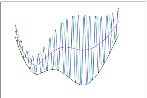
[image:10.595.187.445.325.497.2]

If we consider a sequence of oscillating functionals as in Figure 1.1 we see that although the minimum and minimizers are well behaved the function is not (in the sense that there is no strong limit). And whilst the weak limit exists it clearly does not capture the behavior of either minimizer or minimum. Approximately speaking theΓ-limit is the limiting lower semi-continuous envelope. We see in this case theΓ-limit completely captures the behavior of both the minimum and minimizers. Whilst the example in the figure shows functionals acting on a 1 dimensional space the same reasoning carries through to infinite dimensional spaces.

Figure 1.1: The Weak Limit Versus theΓ-Limit

The blue and green curves show two instances of a minimization problem that becomes increas-ingly oscillatory as the number of data points goes to infinity. The red curve gives the weak limit (i.e. the average over the oscillations) and the black curve is theΓ-limit. Clearly there is no strong limit.

(11)

our framework to investigate the convergence properties for several examples of estimators.

1.2 Overview of Thesis

In this thesis we investigate questions (P1-P2) stated in the previous section for three problems. We give an overview of each type of problem below.

The k-Means Minimization Problem (Chapter 3 and Chapter 4). The first problem we consider is ak-means type problem where we generalize thek-means framework [105] to allow for cluster centers in different spaces to the data. This is motivated by the following smoothing-data association problem. We are given smoothing-data{(ti, zi)}ni=1 sampled fromkunknown curvesµj,

and in particular the association of data point to curve is unknown. The problem is then to recover the set of curves (µ1, . . . , µk) from{(ti, zi)}ni=1. By treating the unknown curves as

cluster centers one can use thek-means method as estimators.

Our setting is we have data ξi ∈ X and cluster centers µj ∈ Y. The cost function

d:X×Y →[0,∞)measures the similarity between a data point and a cluster center. In order for the problem to be well posed we use a regularization termr : Yk → [0,∞) scaled byλ. The object of interest is the optimal cluster centers, that is functionsµ(n)∈Ykthat minimize

fn(µ) =

1

n

X

i=1

min

j=1,...,kd(ξi, µj) +λr(µ).

WhenX =Y we show in Section 3.2 regularization is unnecessary and we can letλ= 0. We prove asymptotics concerning the general case in Chapter 3 before we investigate the smoothing data-association further in Chapter 4 where we also prove a rate of convergence. We definef∞by

f∞(µ) = Z

X

min

j=1,...,kd(x, µj)P(dx) +λr(µ)

and whereξi iid∼ P. Formally, in Chapter 3 we show for sequences of minimizersµ(n) and a

minimizerµ(∞)off∞that:

forX =Y andλ= 0then min

µ∈Xkfn(µ)→_µmin_∈_Xkf∞(µ) µ

(n) _→_µ(∞)

forX 6=Y andλ >0then min

µ∈Ykfn(µ)→_µmin_∈_Ykf∞(µ) µ

(n) _→_µ(∞)

with probability one. And in Chapter 4 we show that:

k

X

j=1 µ

(n)

j −µ

(∞)

j

2

L2 =O

1

n

.

The earliest results regarding the asymptotics of the k-means method considered the application to Euclidean data sets, i.e. X =Y =Rκ andd(x, y) = |x−y|2 where| · |is the

Euclidean norm. Under the assumption that the limiting functionalf∞has a unique minimizer

(12)

results do not hold [19]. With more generality the convergence of the minimum and minimizers for X = Y a reflexive and separable Banach space has been studied in [95, 103]. And an analogous result in [96] for metric spaces. Convergence results forX 6= Y are, as far as the author is aware, new.

The first result known to the author regarding the rate of convergence is a central limit theorem result proved forX = Y = Rκ andd(x, y) = |x−y|2 [126], that is there exists a

covariance matrixΣsuch that

n12

µ(n)−µ(∞)

→N(0,Σ)

where the convergence is in distribution. A simple application of this shows [42] that the mini-mum behaves as

f∞(µ

(n)₎₋_f

∞(µ(n)) =Op

1

n

.

When considering convergence in expectation one has

Ef∞(µ

(n)₎₋_f

∞(µ(∞)) =O

1

√

n

, (1.2)

see for example [10,102,104]. Whenk= 1standard results implyEf∞(µ(n))−f∞(µ(∞)) =

O _n1however whenk≥3it is known [18, 102] that there exists a constantC >0such that

Ef∞(µ

(n)₎₋_f

∞(µ(∞)) ≥

C

√

n

which in particular shows (1.2) is sharp. More generally (1.2) has been shown forX = Y a Hilbert space whend(x, y) =kx−yk2 _and_{k · k}_{is the norm on}_X_{and for}_X ₌_Y _{a separable}

and reflexive Banach space withd(x, y) =kx−yk, see [21, 95] respectively.

General Spline Smoothing (Chapter 5). The second problem, in Chapter 5, looks at the general spline problem. This is similar to the above except we remove the data association problem (i.e. k= 1) and assume there is a true data generating curve. In this case we can scale the regularizationλn→0and recover the ‘truth’ in the data rich limit.

LetHbe a Hilbert space with normk·kand inner product(·,·). We consider the problem of recoveringµ†∈ Hfrom observations{(Li, yi)}ni=1⊂ H∗×Rand the model:

yi =Liµ†+i

whereiis noise. We refer to this as the general spline problem.

A particular case of much interest is whenH =Hm (the Sobolev space of degreem) and observation operators are of the formLiµ=µ(ti). We call this the special spline problem.

We assume that there exists exists a decompositionH=H₀⊕ H₁whereH_iare Hilbert spaces with normsk · ki. The estimatorµ(n)ofµ†is defined to be the minimizer offn :H →

[0,∞)defined by

fn(µ) =

1

n

X

i=1

(13)

whereχ1 :H → H1 is the orthogonal projection. Under suitable conditions one can interpret

µ(n)as a maximum a-posteriori estimator [89]. We assume thatH0is finite dimensional andH1

is infinite dimensional. It is typically not possible to showkµ(n)₋_µ_{k →}₀_{which leaves one}

with two natural options. The first is to look for convergence in a weaker norm, e.g. instead of

Hmwe look atL2, and the second option is to look for weak convergence. Assume thatk · k₁ =kC−1_{· k}

L2 whereCis the covariance operator and the existence of

a compact, positive semi-definite and self-adjoint operatorU which satisfies

1

n

X

i=1

L∗_iLi→U

for some suitable notion of convergence. From the assumptions one has the existence of a eigenbasis{ψi}ofHsatisfying

(ψi, U ψj) =δij and (ψi,C−1ψj) =γiδij.

One then constructs the Hilbert scale by defining the norm

kµkρ=

∞ X

i=1

(1 +γi)ρ(µ, U ψi)2

!1₂

and setsH0

ρ{µ∈ H : kµkρ<∞}. One takesHρto be the completion ofH0ρunderk · kρ. The

main results of [46, 117] imply that

E µ

(n)₋_µ 2

ρ.min

{1, λβ_n−ρ}kµ†k2

β +

1

n(C(λn, ρ) +m)

for any constantβwithρ < β < ρ+ 2, where dim(H0) =mand

C(λ, ρ) = X

j>m

γ_jρ(1 +λγj)−2.

For special splines it has been shown [131, 158] that for uniformly spaced observations the estimateµ(n)ofµ†satisfies the following bound:

E dj dtj(µ

†₋_µ(n)₎ 2 L2

≤A1λ

dj dtjµ

† 2 L2

+ A2

nλ22j+1m

whereA1, A2are constants and0≤j < m. In particular the optimal rate of convergence is for

λnn−

2m

2m+1 _{in which case}

E dj dtj(µ

†₋_µ(n)₎ 2 L2 =O

n−2(m

−j) 2m+1

.

The results also generalize to non-uniform observations under assumptions on the ratio of the largest to smallest gap in observation times [131].

(14)

In particular the result of Chapter 5 is for anyF ∈ H∗ _{and any}_>₀_{we have}

P

F(µ

(n)₎₋_F₍_µ†

)

≥

→0

asn → ∞ when λn = O

1 √

n

, i.e. µ(n) converges weakly and in probability to µ†. As in the strong convergence case we make use of the approximationU ≈ _n1Pn

i=1L ∗

iLi in order to

prove boundedness.

An advantage of our result is that it negates the need for Hilbert scales which can be quite abstruse; by which we mean the spacesHρcan be difficult to identify. Even for Sobolev

spaces understanding Hρ is in general very difficult although for some values of ρ one can

make informative statements such as identifyingH_ρwith another Sobolev space with boundary conditions, see [46, Section 3]. The cost of our approach is that if one wants strong convergence then we are dependent on embedding theorems. Such embedding theorems exist for Hilbert scales but one gets a better rate of convergence (i.e. can scaleλn →0faster) if one proves the

result directly for Hilbert scales rather than proving weak convergence first.

Our results show that for weak convergence one cannot scaleλn → 0 faster that √1_n.

This is natural when one considers weak convergence as a finite dimensional projection and as-sumes a central limit theorem holds. Hence the results of Chapter 5 are optimal and in particular one cannot hope to recover the rates of convergence one has for strong convergence.

A Graphical Approach to Estimating the Data Association (Chapter 6 and Chapter 7).

Chapters 6 and 7 look at the third problem where we use a graphical representation of the data in order to define an estimate to the data association problem, i.e. an estimate ofµ:{0, . . . , n} → {0,1}where for simplicity we assume there are two classes (note the slight change of notation,µ

is now estimating the data association only). We allow for a soft classification so thatµ(j)∈R.

We use minimizers of the Ginzburg-Landau functional which has two terms: the first penalizes soft assignments in order thatµ(j)≈ {0,1}and the second penalizes jumps between adjacent data points soµ(j)≈µ(j+ 1). We use the structure of the graph to determine what data points are adjacent.

To be more precise we look for a functionµ ∈L1(Ψn)whereΨn ={ξi}ni=1 ⊂Rdis

the data and for convenience we writeL1_(Ψ

n)as the set of functions fromΨntoR. The graph

is constructed by weighting edges between pointsξiandξjby

Wij =η(ξi−ξj)

where

η(x) =

1

d n

η

x

is the interaction potential that we scale by=nso that the graph remains sparse. We discuss

(15)

Ginzburg-Landau functionalE_n:L1(Ψn)→[0,∞]by

En(µ) =

1

n n

X

i=1

V(µ(ξi)) +

1

n

1

n2 X

i,j

Wij|µ(ξi)−µ(ξj)|.

We assume thatV(t) = 0⇔ t∈ {0,1}, e.g. V(t) =t2(1−t)2so that the first term penalizes states not taking the values zero or one. The second term is defined as the graph total variation, i.e.

GT Vn(µ) =

1

n

1

n2 X

i,j

Wij|µ(ξi)−µ(ξj)|.

Estimates of the data partition are given by minimizers ofEn.

The asymptotics of the classical Ginzburg-Landau functional (in a continuous setting),

F(µ) =

1

Z

X

V(µ(x)) dx+1

Z

X2

η(x−y)|µ(x)−µ(y)|2 dxdy,

are well known, e.g. [5, 114]. These results show there exists someF0such that

F0 = Γ-lim

→0 F

and for any sequence µ(n) ∈ L1(X) and n → 0 such that supn∈_NFn(µ

(n)₎ _< _∞ _then

{µ(n)}n∈Nis precompact in L1. These results allow one to infer the convergence of the

con-strained minimization problem where the constraints respect theΓ-convergence, see Section 2.2. More recently these results have been extended to discrete settings where{ξi}ni=1form a

regular graph [163]. These results apply when the data is deterministic. The appropriate notion of convergence ofµ(n) → µwhereµ(n) ∈ L1(Ψn)andµ ∈ L1(Rd) is to define a piecewise

constant approximation ofµ(n)onL1(Rd), the details are left to Section 2.5.

For random data points it has been shown in [69] that theΓ-limit of GT Vn is a total

variation distance (whenη is isotropic). A consequence of our results shows this is also true when η is anisotropic. The compactness property for GT Vn requires the sequence µ(n) be

bounded in L1 _and _{GT V}

n in order for compactness in L1 which is easily seen as GT Vn is

invariant underµ7→µ+c.

Our results in Chapter 6 extend [5,163] to show the existence of a surface integral (where we leave the definition until Chapter 6)E∞such thatE∞= Γ-limn→∞Enand the compactness

property holds whenξi

iid

∼ P for a probability measureP. To do so we use the methodology of [69].

The minimization problem,minµEn(µ), admits trivial minimizerµ ≡0orµ ≡ 1. In

order to obtain ‘more interesting’ minimizers one should impose constraints such as the mass constraint, adding a data fidelity term, or boundary conditions. In Chapter 7 we use the results of Chapter 6 to prove convergence results for each of the constrained minimization problems described. To do so one must show that the constraint respects theΓ-convergence. There is also a discussion on the results for more than 2 classes. In Chapters 6 and 7 the data is inRd,

(16)

Chapter 2

Preliminary Material

2.1 Notation

The set of probability measures onXis denotedP(X)and the Borelσ-algebra byB(X). The problems which we address involve random observations usually denotedξi : Ω → X where

we assume throughout the existence of a probability space(Ω,F,P), rich enough to support a

countably infinite sequence of such observations,{ξ(_iω)}∞

i=1. All random elements are defined

upon this common probability space and all stochastic quantifiers are to be understood as acting with respect to P unless otherwise stated. Where appropriate, to emphasize the randomness

of the functionalsfn, we will writefn(ω) to indicate the functional associated with the

partic-ular observation sequenceξ₁(ω), . . . , ξn(ω)and we allowPn(ω)to denote the associated empirical

measure.

For clarity we often write integrals using operator notation. Specifically, for a measure

P (which is usually a probability distribution) we write

P h=

Z

h(x)P(dx).

A sequence of probability distributionsPnon a Polish space is said to converge weakly

to a probability measureP, and we writePn⇒P, if

Pnh→P h for allh∈Cb

where Cb is the space of continuous and bounded functions. A fact we will make use of is

the almost sure weak convergence of the empirical measure, e.g. [56, Theorem 11.4.1]. For a sequenceξ_i(ω)of random variables and each bounded and continuous function,h, it’s possible to define the sequence of random variablesPn(ω)(h)which converges almost surely toP hby the

strong law of large numbers. However this does not immediately imply the almost sure weak convergence of the empirical measure since taking the intersection over the uncountable setCb

does not necessarily have probability one, i.e. we must be careful when concluding the set

Ω0 = \

h∈Cb

n

(17)

has probability one. However, when the spaceXis a separable metric space then one can find a countable dense subset ofCbon which to apply the strong law of large numbers. By a continuity

argument this extends to the whole ofCb.

With a slight abuse of notation we will sometimes writeP(U) :=PIU for a measurable

setU. We denote the support of a probability measureP by supp(P), i.e.

supp(P) = inf

(

X0:X0 ⊂X, X0 is closed, and

Z

X\X0

P(dx) = 0

)

.

Throughout this thesis we say that a sequence of parameter estimators is consistent if, for any value of the “parameters”, they converge with respect to the underlying topology in probability (with respect to the data-generating mechanism) to the true value.

The space of functions fromZ ontoY that areLp-integrable are denoted byLp(Z;Y) (for1 ≤ p ≤ ∞). Usually eitherY = {0,1} orY = R. IfY = R then we write Lp(Z)

instead ofLp(Z;R). When we use theLpnorm with respect to a measureP theY dependence

is suppressed and we writeLp(X;P). It will be obvious from the context what is meant. We define the Sobolev spacesWs,p₍_I₎_on_I _⊆

Rby

Ws,p=Ws,p(I) =

f :I →_Rs.t.∇if ∈Lp(I)fori= 0, . . . , s

where we use∇for the weak derivative, i.e.g=∇f if for allφ∈C_c∞(I)(the space of smooth functions with compact support)

Z

I

f(x)dφ

dx(x)dx=−

Z

I

g(x)φ(x)dx.

In particular, we will use the special case when p = 2 and we write Hs = Ws,2. This is a Hilbert space with norm:

kfk2_Hs =

s

X

i=0

k∇ifk2_L2.

For a Banach spaceAone can define the dual spaceA∗to be the space of all bounded and linear maps overA into Requipped with the norm kFkA∗ = sup_x_∈_A|F(x)|. Similarly

one can define the second dualA∗∗as the space of all bounded and linear maps over A∗ into

R. Reflexive spaces are defined to be spacesAsuch thatAis isometrically isomorphic toA∗∗.

These have the useful property that closed and bounded sets are weakly compact. For example anyLpspace (with1< p <∞) is reflexive, as is any Hilbert space (by application of the Riesz Representation Theorem).

A sequence xn ∈ A is said to weakly convergence tox ∈ A if F(xn) → F(x) for

all F ∈ A∗. We write xn * x. We say a functional G : A → R is weakly continuous

if G(xn) → G(x) wheneverxn * xand strongly continuous if G(xn) → G(x) whenever

kxn−xkA→0. Note that weak continuity implies strong continuity. Similarly a functionalG

is weakly lower semi-continuous iflim infn→∞G(xn)≥G(x)wheneverxn* x.

For a space A and a set K ⊂ A we write Kc _{for the complement of} _K _in _A_{, i.e.}

(18)

For an operatorU :H → Hwe will use Ran(U)to denote the range ofU, i.e.

Ran(U) ={µ∈ H:∃ν ∈ Hs.t.U ν=µ}.

WhenU is linear and(H,k · k)is a Banach space the operator norm is defined by

kUk_L₍_H_,_H₎:= sup

kµk≤1

kU µk.

The Euclidean norm is given by| · |and with a small abuse of notation the dimension is inferred from the argument. The ball centered atxand with radiusrinRdis given as

B(x, r) =ny∈_Rd_:_|_x₋_y_|_{< r}o_.

When the ball is centered at the origin we writeB(0, r).

For two real-valued and positive sequencesanandrnwe writean.rnifa_r_nnis bounded.

If an . rn and rn . an then we write an rn. Alternatively we may sometimes write

an=O(rn)if a_r_nn is bounded whereanandrnare two real valued deterministic sequences and

rn is positive. If a_rn_n → 0asn→ ∞we writean = o(rn). For random sequencesanandrn,

wherern are positive and real valued, we writean = Op(rn)if a_r_nn is bounded in probability:

for all >0there exist deterministic constantsM, Nsuch that

P

an

rn

≥M

≤ ∀n≥N.

If an

rn →0in probability: for all >0

P

an

rn

≥

→0 asn→ ∞

we writean=op(rn).

2.2 Γ

-Convergence

Γ-convergence was introduced in the 1970’s by De Giorgi as a tool for studying oscillatory objects. We are particularly motivated by using theΓ-limit to design our minimization problems so that our classifiers have certain properties. A key contribution of this thesis is to identify the limiting minimization problem associated with a variety of statistical inference problems. Knowledge of the limit aids the practitioner in designing the finite data problem, i.e. allows one to pick out important features of the data. In this senseΓ-convergence is used as a data analysis tool. See, for example [28, 50], for an introduction toΓ-convergence.

We have the following definition ofΓ-convergence, see also Figure 1.1 in Chapter 1 for an illustration ofΓ-convergence.

Definition 2.2.1(Γ-convergence). Let(X, τ) be a topological space. A sequencefn : X →

R∪ {±∞}is said toΓ-converge on the domainXtof∞:X→R∪ {±∞}with respect to the

(19)

(i) (lim inf inequality) for every sequence(ζ(n))converging toζ f∞(ζ)≤lim inf

n→∞ fn(ζ (n)_);

(ii) (recovery sequence) there exists a sequence(ζ(n))converging toζsuch that

f∞(ζ)≥lim sup

n→∞ fn(ζ (n)₎_.

We give the above definition ofΓ-convergence in terms of a general topological space. In this thesis the topology will either be the topology of weak convergence or strong conver-gence.

When it exists theΓ-limit is always lower semi-continuous [27, Proposition 1.31], and hence there exists minimizers over compact intervals. The following result justifies the use of Γ-convergence as a variational type of convergence.

Theorem 2.2.1(Convergence of Minimizers). Let(X, τ)be a topological space andfn:X →

[0,∞]be a sequence of functionals. Letµ(n)be a sequence of almost minimizers offn. Ifµ(n)

are precompact andf∞= Γ-limnfnwheref∞:X →[0,∞]is not identically+∞then

min

X f∞= limn→∞infX fn.

Furthermore any cluster point ofµ(n)_minimizes_f ∞.

A simple consequence of the above is if one can show that the Γ-limit has a unique minimizer then any sequence of almost minimizers converges (without the recourse to subse-quences).

Corollary 2.2.2. If in addition to the assumptions of Theorem 2.2.1 the minimizer of theΓ-limit is unique then any sequence of almost minimizersµ(n)_of_f

nconverges weakly to the minimizer

off∞.

For the Γ-convergence results to carry through to functions on domains fn : Θn →

[0,∞]we require thatΘnare compatible in the following sense.

Definition 2.2.2. Assume thatfnΓ-converges tof∞on a topological space(X, τ). LetΘn,Θ

be subsets ofX. Then we say that(Θn,Θ, fn, f∞)are compatible with respect toΓ-convergence

if

1. Θis closed,

2. there existsζ ∈Θsuch thatf∞(ζ)<∞,

3. ifζ(n)∈Θnandζ(n)→ζthenζ ∈Θand

4. for allµ∈Θthere exists a sequenceµ(n)∈Θnsuch thatµ(n)→µand

lim sup

n→∞ fn(µ

(20)

We immediately see that ifΘn,Θare compatible with respect toΓ-convergence then

fn Γ-converges tof∞ onΘ. Theorem 2.2.1 holds when restrictingfn andf∞ to compatible

subsets.

Corollary 2.2.3. Let(X, τ) be a topological space and fn : X → [0,∞]be a sequence of

functionalsΓ-converging tof∞ : X → [0,∞]. AssumeΘn,Θare compatible with respect to

Γ-convergence. If any sequenceµ(n)of almost minimizers is precompact then

min

Θ f∞= limn→∞infΘn

fn.

Furthermore any cluster point ofµ(n)minimizesf∞inΘ.

Another property ofΓ-convergence we will exploit is it stability under continuous per-turbations. We saygnconverges continuously tog∞ifgn(ζ(n))→g∞(ζ)wheneverζ(n)→ζ.

We have the following proposition.

Proposition 2.2.4. IffnΓ-converges tof∞on a topological space(X, τ)andgncontinuously

converges tog∞then

f∞+g∞= Γ-lim

n→∞ fn+gn.

If gn ≥ 0 then any compactness of fn will also carry through to fn +gn. Hence

convergence of minimizers/convergence of minima results forfncarry through tofn+gn.

2.3 The Gˆateaux Derivative

We very quickly recap Gˆateaux derivatives (also known as directional derivatives) and remind the reader that Taylor’s theorem holds in the multi-dimensional case.

Definition 2.3.1. We say thatf :H →_Ris Gˆateaux differentiable atµ∈ Hin directionν∈ H if the limit

∂f(µ;ν) = lim

r→0

f(µ+rν)−f(µ)

r

exists. We may define second order derivatives by

∂2f(µ;ν, ν0) = lim

r→0

∂f(µ+rν0;ν)−∂f(µ;ν)

r

forµ, ν, ν0 ∈ H. Similarly for higher order derivatives. To simplify notation, when it is clear, we write

∂sf(µ;ν) :=∂sf(µ;ν, . . . , ν).

Theorem 2.3.1(Taylor’s Theorem). Iff :H → _Rism times continuously Gˆateaux differen-tiable on a convex subsetK⊂ Hthen, forµ, ν ∈K:

f(ν) =f(µ) +∂f(µ;ν−µ) + 1 2!∂

2_f₍_µ_;_ν₋_{µ, ν}₋_µ_{) +}_{. . .}

+ 1

(m−1)!∂

m−1_f₍_µ_;_ν₋_{µ, . . . , ν}₋_µ_{) +}_R

(21)

where

Rm(µ, ν−µ) =

1 (m−1)!

Z 1 0

(1−t)m−1∂mf((1−t)µ+tν;ν−µ)dt.

2.4 Total Variation Distance

For the convenience of the reader we define the weighted total variation distance and recall some well known results. We start by defining the total variation distance.

Definition 2.4.1. For a domainX ⊂_Rd_{the weighted total variation}_{T V}₍_·_;_{ρ, η}₎_{of a function}

µ∈L1₍_X₎_{with respect to a density}_ρ_{and potential}_η_{is defined by}

T V(µ;ρ, η) = sup

( Z

X

µ(x) div (φ(x)) dx : φ∈C_c∞(X;Rd),

sup

x∈X

σ∗ −ρ−2(x)φ(x)<∞

)

,

(2.1)

σ∗(φ) = sup

n

ν·φ−σ(ν) : ν ∈_Rdo∈ {0,∞}, (2.2)

σ(ν) =

Z

Rd

η(x)|x·ν|dx. (2.3)

The space of functions with finite weighted total variation is denoted by BV(X;ρ, η). The standard total variation distance onXis defined by

d

T V(µ) = sup

Z

X

µ(x) div(φ) dx : φ∈C_c∞(X),kφk_L∞₍_X₎≤1

.

The standard bounded variation spaceBVd(X)is the set of functions such thatT Vd(µ)<∞.

When µ ∈ L1(X;{0,1}) then one can write the total variation distance as a surface integral. In particular one can write:

T V(µ;ρ, η) =

Z

∂{µ=1}

σ(n(x))ρ2(x) dHd−1(x)

wheren(x)is the outward unit normal for the set ∂{µ = 1}, Hd−1 _{is the} _d₋₁_dimensional

Hausdorff measure. The equivalence whenµ∈L1(X;{0,1})can be seen from the simplifica-tion ofT V(·;ρ, η)whenµ∈C1:

T V(µ;ρ, η) =

Z

X

σ(∇µ(x))ρ2(x) dx=

Z

X

Z

Rd

η(y)|y· ∇µ(x)|ρ2(x) dydx.

One may also write

T V(µ;ρ, η) =

Z

Rd

(22)

whereT Vz(·;ρ)is defined by

T Vz(µ;ρ) = sup

( Z

X

µ(x)div(φ(x)) dx : φ∈C_c∞(X;Rd),

−ν·φ(x)≤ |z·ν|ρ2(x)∀ν, x∈_Rd

) (2.4)

The following proposition is a slight generalization of a well known result regarding the convergence of difference quotients to the total variation semi-norm. The proof is omitted but it is a trivial adaptation of, for example, [97, Theorem 13.48].

Proposition 2.4.1. Assumeµ(n) → µinL1. For a sequencen → 0and a functionρ :X →

[0,∞)definefn:X→[0,∞)by

fn(z) =

1

n

Z

X

µ

(n)₍_x₊

nz)−µ(n)(x)

ρ

2₍_x_{) d}_x.

Then

lim inf

n→∞ fn(z)≥T Vz(µ;ρ).

For eachµ∈BV(X;ρ, η)the following theorem gives the existence of a measure that one can understand as the weak derivative ofµ. See for example [15, 60] for more details.

Theorem 2.4.2. For every µ ∈ BV(X;ρ, η)there exists a Radon measure λρ,η on X and a

λρ,η-measurable functionα:X→Rsuch thatα(x) = 1forλρ,η-almost everyx∈Xand

Z

X

µ(x)divφ(x) dx=−

Z

X

φ(x)·x

ρ2₍_x₎_σ₍_x₎α(x)λρ,η(dx)

for allφ∈C1

c(X;Rd). In particular,

λρ,η(X) =T V(µ;ρ, η).

For the standard total variation distance we writeˆλand have the following relationship:

λρ,η(dx) =ρ2(x)σ(x) ˆλ(dx).

In particular

T V(µ;ρ, η) =

Z

X

ρ2(x)σ(x) ˆλ(dx).

A useful approximation result we will make use of is for allµ ∈ BV(X;ρ, η) there exists a sequenceµ(n)∈BV(X;ρ, η)∩C∞(Rd)such that

µ(n) →µinL1(X) and T V(µ(n);ρ, η)→T V(µ;ρ, η)

or equivalentlyλ(ρ,ηn)(X) → λρ,η(X)(where λ(ρ,ηn) is the measure given by Theorem 2.4.2 and

(23)

The Rellich-Kondrachov theorem implies that any bounded set inBV is relatively com-pact in L1. In particular if a sequence µ(n) can be bounded in BV then one can infer the existence of a subsequence converging inL1_.

2.5 Transportation Theory

In Chapters 6 and 7 we will look for convergence of the data association functionµ : Ψn →

{1, . . . , k}(whereΨn={ξi}ni=1). This requires a notion of convergence suitable for comparing

functions on different domains. We wish to define a mapTn :X → Ψn that will allow us to

extend functionsµ(n)onΨnto functionsµ˜(n)onX, i.e. µ˜(n) =µ(n)◦Tn. The challenge is to

defineTnoptimally in the sense that as little mass as possible is moved. We start by defining

thep-OT distance.

Definition 2.5.1. If1≤p <∞then thep-OT distance betweenP, Q∈ P(X)is defined by

dp(P, Q) = min

( Z

X2

|x−y|p π(dx,dy)

1_p

:π∈Γ(P, Q)

)

(2.5)

whereΓ(P, Q)is the set of couplings betweenP andQ, i.e. the set of probability measures on

X×Xsuch that the first marginal isP and the second marginal isQ. Ifp=∞then the∞-OT distance betweenP, Q∈ P(X)is defined by

d∞(P, Q) = min

ess sup

π

{|x−y|: (x, y)∈X×X}:π∈Γ(P, Q)

. (2.6)

The minimization problem in (2.5) and (2.6) is known as Kantorovich’s optimal trans-portation problem. The minimization is convex and and therefore the minimum is achieved [40, 168]. One can also show that dp defines a metric. Elements π ∈ Γ(P, Q) are called

transference plans. The distance d2 is also known as the Wasserstein metric and d∞ the∞

-transportation distance. For boundedX ⊂ _Rd_{convergence in}_d

p (for1 ≤p < ∞) is

equiva-lent to the weak convergence of probability measures [168] and therefore with probability one,

dp(Pn, P)→0wherePnis the empirical measure.

WhenP has density with respect to the Lebesgue measure then the Kantorovich mini-mization problem is equivalent to the Monge optimal transportation problem [67]:

Minimize

Z

X

|x−T(x)|p _P_(d_x₎ _{over all measurable maps}_T _{such that}_T

#P =Q

where the push forward measure is defined by

T#P(A) =P(T−1(A))

for anyA∈ B(X). IfQ=T#Pthen we callTa transportation map betweenP andQ.

(24)

surely) one can immediately infer the existence of a sequence of transport plans such that

kId−Tnkp_Lp₍_X_;_P₎=

Z

X

|x−Tn(x)|p P(dx)→0 (2.7)

asn→ ∞. We call any sequence of transportation maps{Tn}that satisfy (2.7) stagnating.

In the next definition we use stagnating transport maps to define piecewise constant approximations of functions onΨnin order to define a suitable notion of convergence.

Definition 2.5.2. Letµ(n) ∈ Lp(Ψn) = Lp(X;Pn)andµ ∈ Lp(X;P)We say µ(n) → µin

T Lp(X)if

kµ(n)◦Tn−µkp_Lp =

Z

X

|µ(n)(Tn(x))−µ(x)|p P(dx)→0 (2.8)

for any sequence of stagnating transportation mapsTn :X → Ψn. Similarlyµ(n)is bounded

inT Lp _if_k_µ(n)_◦_T

nkLpis bounded andµ(n)is precompact inT Lp ifµ(n)◦T_nis precompact

inLp.

One can show that if (2.8) holds for one sequence of stagnating transport maps then it holds for any sequence of stagnating transport maps [69, Lemma 3.5].

In Chapters 6 and 7 we will assume thatP has densityρwhich is bounded above and below by positive constants then (2.7) is equivalent tokId−TnkLp₍_X₎ → 0andLp(X;P) =

Lp(X). We will mostly consider the casep = 1however generalizations to 1 < p < ∞ are straightforward.

Now consider an arbitraryT :X →Xand a measurableϕ:X→[0,∞). Recall that

Z

X

ϕ(x)T#P(dx) := sup Z

X

s(x)T#P(dx) : 0≤s≤ϕandsis simple

.

Ifs(x) =PN

i=1aiδUi(x)whereai=s(x)for anyx∈Uithen

Z

X

s(x)T#P(dx) =

N

X

i=1

aiT#P(Ui) = N

X

i=1

aiP(Vi)

forVi =T−1(Ui). Note thatai =s(x)for anyx ∈T(Ui). From this it is not hard to see the

following change of variables formula:

Z

X

ϕ(x)T#P(dx) = Z

X

ϕ(T(x))P(dx). (2.9)

A particularly useful version of this will be whenT#P(dx) =Pn(dx)wherePnis the empirical

measure. In which case (2.9) implies

1

n

X

i=1

ϕ(ξi) =

Z

X

ϕ(T(x))P(dx).

(25)

Lp(Y;Q)whereP, Qare arbitrary measures onXandY respectively. Let us define

dT Lp((P, µ),(Q, ζ)) = inf

π∈Γ(P,Q) (

Z

X×Y

|x−y|pπ(dx,dy)

1

p +

Z

X×Y

|µ(x)−ζ(y)|p π(dx,dy)

1

p

)

.

LetP have density with respect to the Lebesgue measure and take a sequence of measuresPn

defined on a common spaceX(where we do not assume thatPnis the empirical measure). Then

(Pn, fn)→(P, f)inT Lpis equivalent to weak convergence of measures (due to the first term)

andkµ(n)◦Tn−µkLp₍_X_;_P₎→ 0(due to the second term), see [69, Proposition 3.6]. Since we we will always work with the empirical measure then with probability onePnconverges weakly

toP. Hence the first term plays no role in this thesis and so is not included. We recall the following theorem which will be useful later.

Theorem 2.5.1. [70] LetX ⊂_Rd_with_d_≥₂_{be open, connected and bounded with Lipschitz}

boundary. LetP be a probability measure onXwith density (with respect to Lebesgue)ρwhich is bounded above and below by positive constants. Letξ1, ξ2, . . . be a sequence of independent

random variables with distributionP and letPnbe the empirical measure. Then there exists a

constantC >0such that almost surely there exists a sequence of transportation maps{Tn}∞n=1

fromP toPnsuch that

ifd= 2then lim sup

n→∞

√

nkId−TnkL∞₍_X₎

(logn)34

≤C

and ifd≥3then lim sup

n→∞

nd1kId−T_nk_L∞₍_X₎

(logn)1d

(26)

Chapter 3

Convergence of the

k

-Means

Minimization Problem in a General

Setting

Abstract

Thek-means method is an iterative clustering algorithm which associates each ob-servation with one ofkclusters. It traditionally employs cluster centers in the same space as the observed data. By relaxing this requirement, it is possible to apply

thek-means method to infinite dimensional problems, for example multiple target tracking and smoothing problems in the presence of unknown data association. Via

aΓ-convergence argument, the associated optimization problem is shown to con-verge in the sense that both thek-means minimum and minimizers converge in the large data limit to quantities which depend upon the observed data only through

its distribution. The theory is supplemented with two examples to demonstrate the

range of problems now accessible by thek-means method. The first example com-bines a non-parametric smoothing problem with unknown data association. The

second addresses tracking using sparse data from a network of passive sensors.

3.1 Introduction

Thek-means algorithm [105] is a technique for assigning each of a collection of observed data to exactly one ofkclusters, each of which has a unique center, in such a way that each observation is assigned to the cluster whose center is closest to that observation in an appropriate sense.

(27)

In such problems one typically has finite-dimensional data, but would wish to estimate infi-nite dimensional tracks with the added complication of unresolved data association. It is our aim to propose and characterize a framework for thek-means method which can deal with this problem.

A natural question to ask of any clustering technique is whether the estimated clustering stabilizes as more data becomes available. More precisely, we ask whether certain estimates converge, in an appropriate sense, in the large data limit. In order to answer this question in our particular context we first establish a related optimization problem and make precise the notion of convergence.

Consistency of estimators for ill-posed inverse problems has been well studied, for ex-ample [52, 118], but without the data association problem. In contrast to standard statistical consistency results, we do not assume that there exists a structural relationship between the optimization problem and the data-generating process in order to establish convergence to true parameter values in the large data limit; rather, we demonstrate convergence to the solution of a related limiting problem.

This chapter shows the convergence of the minimization problem associated with the

k-means method in a framework that is general enough to include examples where the cluster centers are not necessarily in the same space as the data points. In particular we are moti-vated by the application to infinite dimensional problems, e.g. the smoothing-data association problem. The smoothing-data association problem is the problem of associating data points

{(ti, zi)}ni=1 ⊂[0,1]×Rκ to unknown trajectoriesµj : [0,1] → Rκ forj = 1,2, . . . , k. By

treating the trajectories µj as the cluster centers one may approach this problem using thek

-means methodology. The comparison of data points to cluster centers is a pointwise distance:

d((ti, zi), µj) =|µj(ti)−zi|2(where|·|is the Euclidean norm onRκ). To ensure the problem is

well-posed some regularization is also necessary. Fork= 1the problem reduces to smoothing and coincides with the limiting problem studied in [79]. We will discuss the smoothing-data association problem more in Section 3.3.3.

Let us now introduce the notation for our variational approach. Thek-means method is a strategy for partitioning a data setΨn ={ξi}ni=1 ⊂ Xintokclusters where each cluster has

centerµj for j = 1,2, . . . , k. First let us consider the special case whenµj ∈ X. The data

partition is defined by associating each data point with the cluster center closest to it which is measured by a cost functiond:X×X→[0,∞). Traditionally thek-means method considers Euclidean spacesX = Rκ, where typically we choosed(x, y) = |x−y|2 =Pκi=1(xi−yi)2.

We define the energy for a choice of cluster centers given data by

fn:Xk→R fn(µ|Ψn) =

1

n

X

i=1

k

^

j=1

d(ξi, µj),

where for anykvariables,a1, a2, . . . , ak,

Vk

j=1aj := min{a1, . . . , ak}.The optimal choice of

µis that which minimizesfn(·|Ψn). We define

ˆ

θn= min

(28)

An associated “limiting problem” can be defined

θ= min

µ∈Xkf∞(µ) where we assume thatξi

iid

∼Pfor some suitable probability distribution,P, and define

f∞(µ) = Z k

^

j=1

d(x, µj)P(dx).

In Section 3.2 we validate the formulation by first showing that, under regularity conditions and with probability one, the minimum energy converges: θˆn →θ. And secondly by showing that

(up to a subsequence) the minimizers converge: µ(n) → µ(∞) whereµ(n) minimizesfn and

µ(∞)minimizesf∞(again with probability one).

In a more sophisticated version of the k-means method the requirement thatµj ∈ X

can be relaxed. We instead allow µ = (µ1, µ2, . . . , µk) ∈ Yk for some other Banach space,

Y, and definedappropriately. This leads to interesting statistical questions. WhenY is infinite dimensional even establishing whether or not a minimizer exists is non-trivial.

When the cluster center is in a different space to the data, bounding the set of minimizers becomes less natural. For example, consider the smoothing problem in which one wishes to fit a continuous function to a set of data points. The natural choice of cost function is a pointwise distance of the data to the curve. The optimal solution is for the cluster center to interpolate the data points: in the limit the cluster center may no longer be well defined. In particular we cannot hope to have converging sequences of minimizers.

In the smoothing literature this problem is prevented by using a regularization term

r :Yk →_R. For a cost functiond:X×Y →[0,∞)the energiesfn(·|Ψn), f∞(·) :Yk →R

are redefined

fn(µ|Ψn) =

1

n

X

i=1

k

^

j=1

d(ξi, µj) +λnr(µ)

f∞(µ) = Z k

^

j=1

d(x, µj)P(dx) +λr(µ).

Adding regularization changes the nature of the problem so we commit time in Section 3.3 to justifying our approach. Particularly we motivate treatingλn=λas a constant independent of

n. We are able to repeat the analysis from Section 3.2; that is to establish that the minimum and a subsequence of minimizers still converge.

(29)

strengthened to a central limit theorem in [126] also assuming a unique minimizer to the limiting energy. Other rates of convergence have been shown in [10, 18, 42, 104]. In Hilbert spaces there exist convergence results and rates of convergence for the minimum. In [21] the authors show that|fn(µ(n))−f∞(µ(∞))|is of order √1_n, however, there are no results for the convergence of

minimizers. Results exist fork→ ∞, see for example [34] (which are also valid forY 6=X). Assuming that Y = X, the convergence of the minimization problem in a reflexive and separable Banach space has been proved in [103] and a similar result in metric spaces in [96]. In [95], the existence of a weakly converging subsequence was inferred using the results of [103].

The chapter is structured as follows. In Section 3.2 we consider convergence in the special case when the cluster centers are in the same space as the data points, i.e. Y =X. In this case we don’t have an issue with well-posedness as the data has the same dimension as the cluster centers. For this reason we use energies defined without regularization. Theorem 3.2.5 shows that the minimum converges, i.e. θˆn → θ asn → ∞, for almost every sequence of

observations and furthermore we have a subsequenceµ(nm)_{of minimizers of}_f

nmwhich weakly converge to someµ(∞)which minimizesf∞.

This result is generalized in Section 3.3 to an arbitraryXandY. The analogous result to Theorem 3.2.5 is Theorem 3.3.6. We first motivate the problem and in particular our choice of scaling in the regularization in Section 3.3.1 before proceeding to the results in Section 3.3.2. Verifying the conditions on the cost functiondand regularization termr is non-trivial and so we show an application to the smoothing-data association problem in Section 3.3.3.

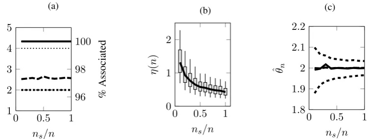
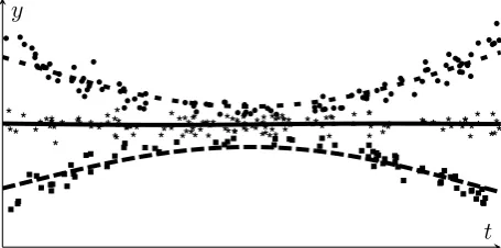
To demonstrate the generality of the results in this chapter, two applications are con-sidered in Section 3.4. The first is the data association and smoothing problem. We show the minimum converging as the data size increases. We also numerically investigate the use of the

k-means energy to determine whether two targets have crossed tracks. The second example uses measured times of arrival and amplitudes of signals from moving sources that are received across a network of three sensors. The cluster centers are the source trajectories inR2.

3.2 Convergence when

Y

=

X

We assume we are given data points ξi ∈ X for i = 1,2, . . . where X is a reflexive and

separable Banach space with normk · kX and Borelσ-algebraX. These data points realize a

sequence ofX-measurable random elements on (Ω,F,P) which will also be denoted, with a

slight abuse of notation,ξi.

We define

f_n(ω):Xk→R, fn(ω)(µ) =Pn(ω)gµ=

1

n

X

i=1

k

^

j=1

d(ξ(_iω), µj) (3.1)

f∞:Xk→R, f∞(µ) =P gµ=

Z

X k

^

j=1

(30)

where

gµ(x) = k

^

j=1

d(x, µj),

Pis a probability measure on(X,X)and the empirical measurePn(ω)associated with{ξ(_iω)}ni=1

is defined by

P_n(ω)h= 1

n

X

i=1

h(ξ(_iω))

for anyX-measurable functionh : X → R. We assumeξi are iid according toP withP =

P◦ξ−i 1.

We wish to show

ˆ

θ_n(ω)→θ for almost everyωasn→ ∞ (3.3) where

ˆ

θ_n(ω)= inf

µ∈Xkf

(ω)

n (µ)

θ= inf

µ∈Xkf∞(µ). We definek · k_k:Xk→[0,∞)by

kµkk := max

j kµjkX forµ= (µ1, µ2, . . . , µk)∈X

k_. _(3.4)

The reflexivity of(X,k · k_X)carries through to(Xk,k · k_k).

Our strategy is similar to that of [124] but we embed the methodology into the Γ-convergence framework. We show that (3.2) is the Γ-limit in Theorem 3.2.2 and that mini-mizers are bounded in Proposition 3.2.3. We may then apply Theorem 2.2.1 to infer (3.3) and the existence of a weakly converging subsequence of minimizers.

The key assumptions ondandP are given in Assumptions 1.1-1.4. The first assump-tion can be understood as a ‘closeness’ condiassump-tion for the spaceX with respect tod. If we let

d(x, y) = 1forx6=yandd(x, x) = 0then our cost functionddoes not carry any information on how far apart two points are. Assume there exists a probability density for P which has unbounded support. Thenfn(ω)(µ) ≥ n−_nk (for almost everyω), with equality when we choose

µj ∈ {ξi(ω)}ni=1. I.e. any set ofkunique data points will minimizef (ω)

n . Since our data points

are unbounded we may find a sequencekξ_i(ω)

n kX → ∞. Now we chooseµ

(n) 1 =ξ

(ω)

in and clearly our cluster center is unbounded. We see that this choice ofdviolates the first assumption. We also add a moment condition to the upper bound to ensure integrability. Note that this also im-plies thatP d(·,0)≤R

XM(kxk) P(dx)<∞sof∞(0)<∞and, in particular, thatf∞is not

identically infinity.

The second assumption is slightly stronger condition on d than a weak lower semi-continuity condition in the first variable and strong semi-continuity in the second variable. The con-dition allows the application of Fatou’s lemma for weakly converging probabilities, see [64].

(31)

fourth implies that we have at leastkopen balls (wherekis known) with positive probability and therefore we are not overfitting clusters to data.

Assumptions 1. We have the following assumptions ond:X×X→[0,∞)andP.

1.1 There exist continuous, strictly increasing functionsm, M: [0,∞)→[0,∞)such that

m(kx−yk_X)≤d(x, y)≤M(kx−yk_X) for allx, y∈X

withlimr→∞m(r) = ∞,M(0) = 0, there exists γ < ∞ such that M(kx+ykX) ≤

γM(kxkX) +γM(kykX)and finally

R

XM(kxkX)P(dx)<∞(andMis measurable).

1.2. For eachx, y∈Xwe have that ifxm →xandyn* yasn, m→ ∞then

lim inf

n,m→∞d(xm, yn)≥d(x, y) and mlim→∞d(xm, y) =d(x, y).

1.3. For eachy∈Xwe have thatd(·, y)isX-measurable.

1.4. There existkdifferent centersµ†_j ∈X,j= 1,2, . . . , ksuch that for allδ >0

P(B(µ†_j, δ))>0 ∀j= 1,2, . . . , k

whereB(µ, δ) :={x∈X :kµ−xkX < δ}.

We now show that for a particular common choice of cost function,d, Assumptions 1.1 to 1.3 hold.

Remark 3.2.1. For anyp >0letd(x, y) =kx−ykp_X thendsatisfies Assumptions 1.1 to 1.3. Proof. Takingm(r) = M(r) = rpwe can boundm(kx−yk_X) ≤ d(x, y) ≤M(kx−yk_X) andm, M clearly satisfym(r) → ∞,M(0) = 0, are strictly increasing and continuous. One can also show that

M(kx+ykX)≤2p−1 kxkp_X +kykp_X

hence Assumption 1.1 is satisfied. Letxm →xandyn* y. Then

lim inf

n,m→∞d(xm, yn) 1

p _{= lim inf}

n,m→∞kxm−ymkX

≥ lim inf

n,m→∞(kyn−xkX− kxm−xkX)

= lim inf

n→∞ kyn−xkX sincexm →x

≥ ky−xk_X

where the last inequality follows as a consequence of the Hahn-Banach Theorem and the fact thatyn−x * y−xwhich implieslim infn→∞kyn−xkX ≥ ky−xkX. Clearlyd(xm, y)→

d(x, y)and so Assumption 1.2 holds.

(32)

We now state the first result of the chapter which formalizes the understanding thatf∞

is the limit offn(ω).

Theorem 3.2.2. Let(X,k·k_X)be a reflexive and separable Banach space with Borelσ-algebra, X; let{ξi}i∈Nbe a sequence of independentX-valued random elements with common lawP.

Assume d : X ×X → [0,∞) and thatP satisfies the conditions in Assumptions 1. Define

fn(ω):Xk→Randf∞:Xk→Rby(3.1)and(3.2)respectively. Then

f∞= Γ-lim

n f

(ω)

n

forP-almost everyω.

Proof. DefineΩ0 as the intersection of three events:

Ω0=

(

ω∈Ω :P_n(ω)⇒P

)

∩

(

ω∈Ω :P_n(ω)(B(0, q)c)→P(B(0, q)c)∀q ∈_N

)

∩

(

ω ∈Ω :

Z

X

IB(0,q)c(x)M(kxk_X)P_n(ω)(dx)

→

Z

X

IB(0,q)c(x)M(kxk_X)P(dx)∀q∈_N

)

.

By the almost sure weak convergence of the empirical measure [56] the first of these events has probability one, the second and third are characterized by the convergence of a countable collection of empirical averages to their population average and, by the strong law of large numbers, each has probability one. HenceP(Ω0) = 1.

Fixω ∈ Ω0: we will show that the lim inf inequality holds and a recovery sequence exists for this ω and hence for every ω ∈ Ω0. We start by showing the lim inf inequality, allowing{µ(n)}∞_n₌₁ ∈Xkto denote any sequence which converges weakly toµ∈Xk. We are required to show:

lim inf

n→∞ f (ω)

n (µ(n))≥f∞(µ).

By Theorem 1.1 in [64] we have

Z

X

lim inf

n→∞,x0_→_xgµ(n)(x

0₎_P_(d_x₎_≤_{lim inf}

n→∞ Z

X

g_µ(n)(x)P_n(ω)(dx) = lim inf

n→∞ P (ω)

n gµ(n).

For eachx∈X, we have by Assumption 1.2 that

lim inf

x0_→_x,n_→∞d(x 0_{, µ}(n)

j )≥d(x, µj).

By taking the minimum overjwe have

lim inf

x0_→_x,n_→∞gµ(n)(x 0_{) =}

k

^

j=1

lim inf

x0_→_x,n_→∞d(x 0_{, µ}(n)

j )≥ k

^

j=1

d(x, µj) =gµ(x).

Hence

lim inf

n→∞ f (ω)

n (µ(n)) = lim inf_n_→∞ Pn(ω)gµ(n) ≥ Z

X

(33)

as required.

We now establish the existence of a recovery sequence for everyω∈Ω0and everyµ∈

Xk_{. Let}_µ(n) ₌_µ _∈_Xk_{. Let}_ζ

qbe aC∞(X)sequence of functions such that0 ≤ζq(x) ≤1

for allx∈X,ζq(x) = 1forx∈B(0, q−1)andζq(x) = 0forx6∈B(0, q). Then the function

ζq(x)gµ(x)is continuous inx(and with respect to convergence ink · kX) for allq. We also have

ζq(x)gµ(x)≤ζq(x)d(x, µ1)

≤ζq(x)M(kx−µ1kX)

≤ζq(x)M(kxkX +kµ1kX)

≤M(q+kµ1kX)

soζqgµis a continuous and bounded function, hence by the weak convergence ofPn(ω)toP we

have

P_n(ω)ζqgµ→P ζqgµ

asn→ ∞for allq ∈_N. For allq∈_Nwe have

lim sup

n→∞

|P_n(ω)gµ−P gµ| ≤lim sup n→∞

|P_n(ω)gµ−Pn(ω)ζqgµ|+ lim sup n→∞

|P_n(ω)ζqgµ−P ζqgµ|

+ lim sup

n→∞

|P ζqgµ−P gµ|

= lim sup

n→∞

|P_n(ω)gµ−Pn(ω)ζqgµ|+|P ζqgµ−P gµ|.

Therefore,

lim sup

n→∞

|P_n(ω)gµ−P gµ| ≤lim sup

q→∞ lim supn→∞

|P_n(ω)gµ−Pn(ω)ζqgµ|

by the dominated convergence theorem. We now show that the right hand side of the above expression is equal to zero. We have

|P_n(ω)gµ−Pn(ω)ζqgµ| ≤Pn(ω)I(B(0,q−1))cg_µ

≤P_n(ω)I(B(0,q−1))cd(·, µ₁)

≤P_n(ω)I(B(0,q−1))cM(k · −µ₁k_X)

≤γP_n(ω)I(B(0,q−1))cM(k · k_X) +M(kµ₁k_X)P_n(ω)_I₍_B₍₀_,q₋₁₎₎c

→γ PI(B(0,q−1))cM(k · k_X) +M(kµ₁k_X)P_I₍_B₍₀_,q₋₁₎₎c asn→ ∞

→0 asq → ∞

where the last limit follows by the monotone convergence theorem. We have shown

lim

n→∞|P (ω)

n gµ−P gµ|= 0.

Hence

(34)

as required.

Now we have established almost sureΓ-convergence we establish the boundedness con-dition in Proposition 3.2.3 so we can apply Theorem 2.2.1.

Proposition 3.2.3. Assuming the conditions of Theorem 3.2.2 and definek · k_kby(3.4), there existsR >0such that

inf

µ∈Xkf

(ω)

n (µ) = inf

kµkk≤R

f_n(ω)(µ) ∀nsufficiently large forP-almost everyω. In particularRis independent ofn.

Proof. The structure of the proof is similar to [96, Lemma 2.1]. We argue by contradiction. In particular we argue that if a cluster center is unbounded then in the limit the minimum is achieved over the remainingk−1cluster centers. We then use Assumption 1.4 to imply that adding an extra cluster center will strictly decrease the minimum, and hence we have a contra-diction.

We defineΩ00to be

Ω00=∩_δ_∈_Q_∩₍₀_,_∞₎_,l₌₁_,₂_,...,knω∈Ω0 :P_n(ω)(B(µ†_l, δ))→P(B(µ†_l, δ))o.

AsΩ00is the countable intersection of sets of probability one, we haveP(Ω00) = 1. Fixω ∈Ω00

and assume that the cluster centersµ(n) _∈_Xk_{are almost minimizers, i.e.}

f_n(ω)(µ(n))≤ inf

µ∈Xkf

(ω)

n (µ) +εn

for some sequenceεn>0such that

lim

n→∞εn= 0. (3.5)

Assume that lim

n→∞kµ (n)_k

k = ∞. There existsln ∈ {1, . . . , k}with lim n→∞kµ

(n)

ln kX =

∞. Fixx∈Xthen

d(x, µ(_ln)

n )≥m(kµ

(n)

ln −xkX)→ ∞. Therefore, for eachx∈X,

lim

n→∞  

k

^

j=1

d(x, µ(_jn))− ^

j6=ln

d(x, µ(_jn))

 = 0.

Letδ >0then there existsN such that forn≥N

k

^

j=1

d(x, µ(_jn))− ^

j6=ln

(35)

Hence lim inf n→∞ Z   k ^ j=1

d(x, µ(_jn))− ^

j6=ln

d(x, µ(_jn))



 P_n(ω)(dx)≥ −δ.

Lettingδ →0we have

lim inf n→∞ Z   k ^ j=1

d(x, µ(_jn))− ^

j6=ln

d(x, µ(_jn))



 P_n(ω)(dx)≥0

and moreover

lim inf

n→∞

f_n(ω)µ(n)−f_n(ω)(µ(_jn))j6=ln

≥0, (3.6)

where we interpretfn(ω)accordingly. It suffices to demonstrate that

lim inf

n→∞

inf

µ∈Xkf

(ω)

n (µ)− inf µ∈Xk−1f

(ω)

n (µ)

<0. (3.7)

Indeed, if (3.7) holds, then

lim inf

n→∞

f_n(ω)µ(n)−f_n(ω)(µ(_jn))j6=ln

= lim

n→∞ f (ω)

n

µ(n)− inf

µ∈Xkf

(ω)

n (µ)

| {z }

≤εn

+ lim inf

n→∞

inf

µ∈Xkf

(ω)

n (µ)−fn(ω)

(µ(_jn))j6=ln

<0 by (3.5) and (3.7),

but this contradicts (3.6).

We now establish (3.7). By Assumption 1.4 there existskcentersµ†_j ∈ Xandδ1 > 0

such thatminj6=lkµ

†

j −µ

†

lkX ≥ δ1. Hence for anyµ ∈ Xk

−1 _{there exists}_l _{∈ {}₁_,₂_{, . . . , k}_}

such that we have

kµ†_l −µjkX ≥

δ1

2 forj= 1,2, . . . , k−1.

Proceeding with this choice ofl, forx∈B(µ†_l, δ2)(for anyδ2 ∈(0, δ1/2)) we have

kµj−xkX ≥

δ1

2 −δ2

and therefored(µj, x)≥m(δ₂1 −δ2)for allj= 1,2, . . . , k−1. Also

Dl(µ) := min

j=1,2,...,k−1d(x, µj)−d(x, µ †

l)≥m(

δ1

2 −δ2)−M(δ2). (3.8)

So forδ2sufficiently small there exists >0such that

Variational methods for geometric statistical inference

University of Warwick institutional repository:

http://go.warwick.ac.uk/wrap

A Thesis Submitted for the Degree of PhD at the University of Warwick

http://go.warwick.ac.uk/wrap/74241

This thesis is made available online and is protected by original copyright.

Please scroll down to view the document itself.

Variational Methods For Geometric Statistical Inference

Matthew Thorpe

Mathematics Institute

Contents

Acknowledgments

Declarations

Abstract

Chapter 1

Introduction

1.1

Motivation

1.2

Overview of Thesis

Chapter 2

Preliminary Material

2.1

Notation

2.2

Γ

-Convergence

2.3

The Gˆateaux Derivative

2.4

Total Variation Distance

2.5

Transportation Theory

Chapter 3

Convergence of the

k

-Means

Minimization Problem in a General

Setting

3.1

Introduction

3.2

Convergence when

Y

=

X