warwick.ac.uk/lib-publications
Original citation:
Irvine, Michael Alastair, Bull, J. C. and Keeling, Matthew James. (2015) Aggregation dynamics explain vegetation patch-size distributions. Theoretical Population Biology, 108 . pp. 70-74.
Permanent WRAP URL:
http://wrap.warwick.ac.uk/79250
Copyright and reuse:
The Warwick Research Archive Portal (WRAP) makes this work by researchers of the University of Warwick available open access under the following conditions. Copyright © and all moral rights to the version of the paper presented here belong to the individual author(s) and/or other copyright owners. To the extent reasonable and practicable the material made available in WRAP has been checked for eligibility before being made available.
Copies of full items can be used for personal research or study, educational, or not-for-profit purposes without prior permission or charge. Provided that the authors, title and full bibliographic details are credited, a hyperlink and/or URL is given for the original metadata page and the content is not changed in any way.
Publisher’s statement:
© 2016, Elsevier. Licensed under the Creative Commons Attribution-NonCommercial-NoDerivatives 4.0 International http://creativecommons.org/licenses/by-nc-nd/4.0/
A note on versions:
The version presented here may differ from the published version or, version of record, if you wish to cite this item you are advised to consult the publisher’s version. Please see the ‘permanent WRAP URL’ above for details on accessing the published version and note that access may require a subscription.
Aggregation dynamics explain vegetation patch-size
distributions
MA. Irvinea,∗, JC. Bullb, MJ. Keelinga
aCentre for Complexity Science, University of Warwick, Coventry, CV4 7AL, UK. bDepartment of Biosciences, Wallace Building, Swansea University, Swansea, SA2 8PP,
UK.
Abstract
Vegetation patch-size distributions have been an intense area of study for theoreticians and applied ecologists alike in recent years. Of particular inter-est is the seemingly ubiquitous nature of power-law patch-size distributions emerging in a number of diverse ecosystems. The leading explanation of the emergence of these power-laws is due to local facilitative mechanisms. There is also a common transition from power law to exponential distribution when a system is under global pressure, such as grazing or lack of rainfall. These phenomena require a simple mechanistic explanation. Here, we study vege-tation patches from a spatially implicit, patch dynamic viewpoint. We show that under minimal assumptions a power-law patch-size distribution appears as a natural consequence of aggregation. A linear death term also leads to an exponential term in the distribution for any non-zero death rate. This work shows the origin of the breakdown of the power-law under increasing pressure and shows that in general, we expect to observe a power law with an exponential cutoff (rather than pure power laws). The estimated param-eters of this distribution also provide insight into the underlying ecological mechanisms of aggregation and death.
Keywords: patch-size distribution, pattern formation, spatial ecology, aggregation
∗Corresponding author.
1. Introduction 1
Vegetation patch-size distributions have been under intense study in re-2
cent years [1, 2, 3, 4, 5]. It has been shown that a power-law provides a 3
good fit to the patch-size distribution under a robust range conditions, how-4
ever there are marginal cases to this. K´efi et al. [6] analysed patch-size 5
distributions in semi-arid vegetation in the Mediterranean and found that 6
there was not only a power-law distribution evident in the patch-size distri-7
bution, but also a truncated exponential term, when the system was under 8
increased grazing pressure. Similar power-law distribution phenomena have 9
also been detected in a number of other ecosystems including mussel beds 10
[7] and marine benthic diatoms [8]. This phenomena of a power-law distri-11
bution transitioning to an exponential distribution under increasing stress 12
has recently shown to be robust, where diverse ecological models are able to 13
reproduce these results [2]. 14
The leading explanation of this power-law pattern formation in ecology 15
is due to local interactions driving the large-scale behaviour [9, 10]. Scanlon 16
et al. [11] supported through the use of numerical simulation of spatially-17
explicit models of vegetation growth combined with a global effect on the 18
population density interpreted as the amount of rainfall or other global pro-19
cesses. The local positive feedback process driving the patch formation is 20
through facilitation of neighbourhood sites that increase the birth rate and 21
decrease the death rate [5]. This explanation does not answer how a power-22
law forms at the patch level, whether it is due to a competition effect between 23
larger clusters dominating the landscape or an aggregation of smaller clus-24
ters. There is also an open question of how patches aggregating together 25
drives these observed patterns. 26
Models of aggregation and fragmentation have been considered in other 27
areas in ecology such as the size of fish schools [12] and marine diatoms [13]. 28
Aggregation phenomena has been more generally studied in the Physical sci-29
ences [14], including processes such as polymerisation [15], coagulation of 30
aerosols [16] and flocculation [17]. Although these examples include clusters 31
that may diffuse, aggregation phenomena may also be considered in the case 32
where clusters are immobile [18]. Aggregation of vegetation clusters, how-33
ever, has not been previously considered as an explicit driving force of the 34
evolution of the patch-size distribution. Our novel contribution here is to 35
apply established theory of aggregation dynamics to the system of vegeta-36
is applicable to vegetation dynamics. 38
In this article, spatially implicit models of vegetation clusters are investi-39
gated by considering how patches form and aggregate. The general conditions 40
under which a power-law distribution is expected to emerge are explored as 41
well as when there is a breakdown of the power law distribution due to an ex-42
ponential truncation. By adopting a patch-centric viewpoint, the impact of 43
aggregation on the resulting distribution along with other processes may be 44
studied directly. This represents a powerful new approach to understanding 45
the origin of these distributions, by explicitly modelling the patch-size dy-46
namics without the need to infer the patch-size distribution from a spatially 47
explicit model [5]. 48
Further, the connection between the power-law exponent and the persis-49
tence of the distribution in this model is explored. We begin by defining a 50
novel model of aggregation with linear death and then deriving an asymp-51
totic solution when the death rate is small.This analytic result is compared 52
to a simulation study of vegetation with local and global growth properties 53
subjected to a global disturbance. For small disturbance, the power law ex-54
ponent closely matches the exponent expected from the model. The conclu-55
sion is that the power-law clustering observed in many vegetation ecosystems 56
may simply be an aggregation effect and the exponential truncation observed 57
when there is increased stress is due to an increase in the linear death rate 58
of clusters. 59
2. Theory 60
The idea developed here is to model the patches themselves as opposed 61
to an individual spatial site as is done in probabilistic cellular automata 62
[19, 20]. We denote ck(t) as the density of patches of sizek at timet, where 63
time is taken to be continuous. A continuous model of patch-sizes can be 64
studied, however for the present k shall take positive integer values only, 65
k ∈ {1,2, . . .}. A kernel of aggregation gives the rate at which patches of
66
size i and j aggregate together to form a patch of size i +j, this kernel 67
is denoted K(i, j). Finally it is assumed there is a constant rate at which 68
patches of size 1 or monomers enter the system. These assumptions are 69
general and can include many different phenomena, including static clusters 70
the Smoluchowski equation [21] is then 72
d dtck =
1 2
X
i+j=k
K(i, j)cicj −
X
j≥1
K(j, k)cjck+δk,1, (1)
where δk,1 is the Kronecker-delta function that is 1 when k = 1 and 0 other-73
wise. For convenience, time has been re-scaled such that the rate at which 74
aggregation occurs is 1. It is instructive to imagine a single unit or monomer 75
coming into contact with a cluster and calculating the rate at which this oc-76
curs for larger as opposed to smaller clusters. Ifa >0 then, assuming the size 77
of the monomer is negligible, the monomer rate equation is K(i) =i−a. This 78
means smaller clusters are favoured and the growth rate reduces as clusters 79
grow larger in size. An ecological explanation of this could be due to the 80
self-limitation through competition a larger cluster experiences with itself, 81
thus reducing its potential for growth. Smaller clusters have more space and 82
thus can grow at a quicker rate. 83
When a < 0, larger clusters are favoured for growth compared with
84
smaller clusters, this can be seen as a form of the Allee effect [22]. In the 85
regime when a < 0, small clusters are more susceptible to environmental 86
perturbation and as such, have a lower propensity for growth. At the other 87
length scale, larger clusters of vegetation are able to regulate their environ-88
ment more and thus have greater resources for growth (An example species 89
where this holds is ribbed mussels [23], where larger clusters provide protec-90
tion and shelter for new mussels). This example of an Allee effect can be 91
demonstrated by again considering the rate at which single units of vegetation 92
aggregate to a cluster. If ai > j, then K(1, i) = 1 +i−a>1 +j−a =K(1, j) 93
i.e. the rate at which a larger patch recruits new growth is greater than for a 94
smaller patch. A value for a then can give an indication of whether there is 95
strong small cluster growth at the expense of large clusters forming or if the 96
converse holds. 97
An alternative explanation of the aggregation exponent a is due to the 98
edge effects of a cluster. A single individual vegetation unit aggregates to a 99
cluster proportional to the edge of that cluster. If all clusters are non-fractal 100
then it would be expected that a vegetation unit aggregates at ratei1/2, since 101
the length of a non-fractal object scales as a square root with its area. For 102
a general fractal cluster with boundary dimension d, it would be expected 103
that an individual unit scales as i1/d. 104
Various properties are desirable for the kernel. Firstly symmetry, where 105
ordering of the patches i.e. K(i, j) =K(j, i). Secondly, scaling homogeneity, 107
where the rate at which patches of a certain size aggregate scales by some 108
factor K(mi, mj) =mλK(i, j). The simplest kernel that satisfies these con-109
ditions is the constant kernel K(i, j) = 1, corresponding to the case where 110
λ = 0. When this form of kernel is assumed, the tail-solution (for large k) 111
has the simple form [24] 112
ck∼ 1 √
4π 1
k3/2. (2)
The tail of the patch-size distribution is a power law with exponent 3/2, 113
where the power law nature of the solution is a consequence of the injection 114
term ( where births of patch size one enter the system ) and the non-linear 115
aggregation term in the equation. The equation can be solved analytically 116
for more general kernels of the type 117
K(i, j) = i−a+j−a. (3)
118
This type of kernel also admits an analytic solution in the large patch-size 119
limit [25, 26] with a steady state distribution of the form where 120
ck∼Ck−τ (4a)
τ = 3−a
2 , C =
r
1−a2 4π cos
πa
2
. (4b)
For a steady state to exist we require −1 < a < 1 and hence the scaling 121
exponent can be found on the interval τ ∈ (1,2). The dynamics of the 122
equation can be assessed by defining the cross-over time, which is the time 123
taken for a density of patches of a certain size to reach its asymptotic value. 124
The cross-over time for a patch of size k∗ to the steady state solution ck∗ 125
is found to take the form t = (k∗)z where z = (1 +a)/2. The scaling of 126
the cross-over time and the patch-size exponent can be related by the simple 127
linear equation τ = 2−z. This gives a linear relationship between the static 128
exponent at stationarity and its dynamic exponent. 129
A real vegetation system is not purely defined by an aggregation process 130
however. In particular in the previous example there is no death either of 131
single vegetation units or patch clusters. Death may lead to changes in the 132
exponent of the stationary distribution and so it is important to include in 133
any model of vegetation clustering. It is also assumed that a death event does 134
with a linear death term can then be produced as 136
d dtck =
1 2
X
i+j=k
K(i, j)cicj−
X
j≥1
K(j, k)cjck+µ(k+ 1)ck+1−µ(k)ck, (5a)
d
dtc1 =−
X
j≥1
K(j,1)cjc1+ 1 +µ(2)c2−µ(1)c1. (5b)
The general additive aggregation kernel is again taken to be of the form 137
K(i, j) = i−a+j−a, where a represents the scaling parameter of the rate at 138
which aggregates of a certain size join. If it is equally likely for a cluster 139
of a certain size to aggregate with a cluster of any other size then the scale 140
parameter a= 0. For a pure aggregation system with no fragmentation, this 141
leads to a cluster scaling of 3/2. µ(k) defines the death rate, which is the 142
rate at which individual units are lost from a patch, where a patch of size k 143
transitions to a patch of size k−1 due to exogenous or endogenous factors. 144
A number of different forms of this death rate may be considered dependent 145
on the biological details of the system. For example if each individual has a 146
constant rate of death regardless of the size of patch its contained, such as due 147
to lack of rainfall or grazing, is then µ(k) =µk. If death occurs at the edge 148
of a patch then the death rate is µk1/d, where d is the boundary dimension 149
of the patches. The simplest form of the death rate is where µ(k) = µ for 150
all k. In order to gain insight into the effect of a death rate on the resulting 151
patch-size distribution, we assume the final form of the death rate. 152
In order to gain analytic tractability on the model a constant aggregation 153
kernel is assumed (a= 0, K = 2) together with a constant death rate for each 154
individual within a patch. The strategy for deriving a solution is similar to 155
the strategy in Krapivsky et al. [26]. A constant kernel K(i, j) = 2 is used. 156
Eq. (5) is rewritten as 157
d dtck =
X
i+j=k
cicj−2ck
X
j≥1
cj+µck+1−µck, (6a)
d
dtc1 =−2c1
X
j≥1
cj + 1 +µc2−µc1. (6b)
The asymptotic tail of the resulting patch-size distribution is then sought 158
in order to gain an understanding of how the linear death rate affects the 159
stationary distribution. By using the asymptotic approximation and assum-160
patches of size k is 162
ck =k−3/2exp(−Λk), (7)
where Λ = log(1 +µN) and N is the total population size (See Appendix A 163
for a derivation). The solution is therefore a power law with an exponential 164
truncation of factor Λ. When the death rate is 0, Λ = 0 and hence the patch-165
size distribution is a pure power law as is expected. A large death rate will 166
lead to a solution that is dominated by an exponential decay term, hence the 167
patch-size distribution is expected to have a smooth transition from a pure 168
power law to an exponential distribution. A dimensionality argument of Eq. 6 169
[27] also leads to a power law exponent of the form 3/2. This solution can 170
be compared to the general power-size distribution with exponential cut-off 171
N(k) given by 172
N(k) =Ck−αexp(−k/kx), (8)
173
wherekx is the patch-size above whichN(s) decreases faster than power-law 174
[2]. Matching terms and assuming µN is small gives the following simple 175
relationship between the cross-over patch size kx and death rate µ as 176
kx = 1
N µ. (9)
177
The model therefore predicts an inverse relationship between patch-size cross-178
over and death rate. This also predicts that when the death rate is small 179
enough, the cross-over patch-size kx may be larger than the system size and 180
as such the exponential tail may not be observed in empirical distributions. 181
3. Results 182
In order to compare the model predictions of patch formation in an aggre-183
gation system with a constant death rate to the prediction of the patch-size 184
distribution obtained in Eq. 7 is compared to a simple probabilistic cellu-185
lar automata model of vegetation growth. The cellular model is similar to 186
the one discussed in [11], the model is defined on a toroidal lattice where 187
each site can exist in one of two states: occupied (1) and empty (0). The 188
occupied state propagates through nearest neighbour growth at rate β, as 189
well as through a background constant birth probability γ. The alive sites 190
transition to a dead site with a constant death probability µ. Hence if nx is 191
be summarised as 193
Px(0→1) =min{1, γ+βnx/4}, (10a)
Px(1→0) =µ, (10b)
where sets the total reaction rate of the system and was implemented to 194
reduce the probability of multiple events occurring within the same neigh-195
bourhood. The minimum function is used here to guarantee the probability 196
of transitioning to an alive state is one in the rare case when the sum of the 197
two probabilities increases above one. 198
Simulations were conducted for constant local growth, birth rate and 199
reaction rate β = 0.2, γ = 0.01, = 0.1 and over a range of death rates. 200
Simulations were ran for lattice lengthL= 500 and for 1000 replicates of each 201
parameter set. The patch-size distribution was recorded for each simulation 202
run after 600 time-steps. This was chosen so that when µ = 0, the lattice 203
is approximately 50% occupied. The following power-law with exponential 204
truncation was fitted to the distribution using a maximum likelihood method 205
f(K =k) =Ck−αexp(−Λk), (11)
for some normalising factor C. The resulting maximum likelihood estima-206
tors were found using a downhill simplex method implemented in Matlab 207
R2014a [28]. The approximate solution to the aggregation equation predicts 208
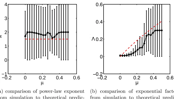
a constant power-law exponent α of 3/2. This is close to the inferred value 209
from simulation for the range of µvalues studied (Fig. 1a). The exponential 210
factor Λ is zero when the death rate is zero (Fig. 1b), as predicted. For 211
increasing death rate, Λ increases again as predicted. Overall there is an 212
increase in the exponential factor for increasing death rate as is predicted, 213
however the functional form of the increase is not fully captured by the mean 214
field approximation. 215
4. Discussion 216
Changing the focus away from explicit spatial modelling of vegetation 217
patch formation and instead focusing on the dynamics of patch-sizes gives a 218
unique insight into the underlying aggregation-fragmentation processes. Here 219
we have primarily focused on solutions to equations where the aggregation 220
−0.2 0 0.2 0.4 0.6 −1
0 1 2 3 4
µ α
(a) comparison of power-law exponent from simulation to theoretical predic-tion
−0.2 0 0.2 0.4 0.6
−0.2 0 0.2 0.4 0.6
µ
λΛ
[image:10.612.120.489.130.341.2](b) comparison of exponential factor from simulation to theoretical predic-tion
Figure 1: Exponents of patch-size distribution compared to simulations. Theoretical values shown as red dashed lines, while simulation calculated values are given as black dots with 95% confidence intervals. The theoretical values for the power-law exponent α and the exponential factor Λ are derived in Eq. 7. As predicted for small values of the death rate the power-law component of the patch-size distribution is constant whilst there is an increase in the exponential component for increasing death rate.
either a constant or power law kernel. For a system where there is aggrega-222
tion only the resulting patch-size distribution is that of a pure power law, 223
with exponent that is dependent on the exponent of the power law aggrega-224
tion kernel. The introduction of a linear death term, where an individual is 225
lost from a patch at rate µ/k gives rise to a power law with exponential tail 226
distribution of the form ck ∼ k−αexp(−Λk). This solution holds generally 227
when there is a linear death term and power-law aggregation kernel, even 228
when the kernel is composed of a sum of two power-laws. Further, α is de-229
pendent on the specifics of the aggregation term alone and Λ is dependent on 230
the death rate alone. This separation of the aggregation and fragmentation 231
term implies, in principle, the ability to infer aggregation and death processes 232
through observing the converged patch-size distribution alone, hence this is 233
K´efi et al. [6, 2] predicts that a power-law distribution in the patch-size 235
distribution occurs when a global environmental death rate is small. This 236
transitions to an exponential distribution when there is greater stress on the 237
system through this global death rate term. The model used is a spatially-238
explicit one with a local growth term and a background death rate. The 239
model proposed in this article can be seen as a deterministic equivalent of 240
this spatially-explicit model. Through the derived solution in this article it is 241
observed that there should always be an exponential tail to the distribution 242
if the death rate is non-zero. Similar arguments have also been made recently 243
[29], but notably none have explained the origin of a power law with exponen-244
tial tail observed in vegetation systems. The derived model then, provides a 245
theoretical origin to the observed spatial patterns in vegetation ecosystems 246
that are under a pressure that can be considered constant throughout space 247
(rainfall, grazing etc.). As an example, if all sites had the same death rate 248
regardless of its neighbourhood, such as for a grazer, the death rate would 249
be µk for a patch of size k. The model also suggests that a power-law with 250
exponential tail is a more accurate description of the patch-size distribution, 251
although when the death rate is small, the exponential tail may not be ob-252
served directly. This approach would be able to provide further insights into 253
the nature of the patch-size distribution for other systems where disturbance 254
may be spatially distributed. 255
The model also gives insight into how there can be a continuous array 256
of power-law exponent observed in nature. The aggregation with no death 257
model predicts that power-laws exponents in the range (1,2) are physically 258
possible, which is what has been observed in a number of ecosystems [7, 6, 8]. 259
The model predicts that a change in the exponent of a patch-size distribu-260
tion is related to a change in the power-law exponent of the aggregation 261
kernel. A simple dimensionality argument can be used to show that in the 262
aggregation and death model with a kernel that has a general power law 263
scaling as described in Eq. 3, the resulting stationary distribution will have 264
the same exponent as that in the model with no death [27]. The conclusion 265
of how to relate the patch-size distribution to the system dynamics is that 266
both the power-law exponent and the presence of an exponential cut-off does 267
give an indication of the underlying dynamics. More complex fragmentation 268
processes than the one discussed would alter these conclusions however, as a 269
non-linear fragmentation process will also lead to self-similar solutions and 270
thus the two processes are confounded when only the stationary state is ob-271
that could split a single cluster of vegetation into multiple clusters. The size 273
of the system where the dynamics occur, such as in the lattice model, may 274
also have an impact on the exponents of the patch-size distribution due to 275
finite-size effects [31]. 276
Other possible extensions to the model could include multi-species sys-277
tems, where patches are formed of multiple species each with their own in-278
trinsic death rates. Multi-species systems have already been considered in 279
the physical sciences and as such this would make for an interesting avenue of 280
future research [32]. Where the aggregation process is indistinguishable be-281
tween two different species, this leads to similar results laid out in this article 282
[33]. However, more complex interactions such as inter-specific competition 283
would inevitably lead to a more complex relationship between the exponent 284
death term and the underlying death rates. The model equations were scaled 285
such that the rate of aggregation and rate at which single vegetation units 286
are created is one. This was done for convenience since we were interested in 287
studying the scaling alone, whereas these parameters change the constant of 288
the patch-size distribution only. Another extension then would be to explic-289
itly calculate the constant for the patch-size distribution and study how this 290
changes as the other system rates change. 291
Acknowledgement 292
The work conducted in this article was funded as part of an EPSRC 293
studentship. 294
Appendix A. Derivation of asymptotic solution 295
A moment-generating function is used to find the steady state solution 296
to this equation in a similar fashion to the one described in Krapivsky et al. 297
[26]. Firstly define the total number of all patches as N =P
k≥1ck and then 298
sum Eq. (6a-b) in order to obtain 299
dN
dt =
X
k≥1
X
i+j=k
cicj−2
X
k≥1 ck
X
j≥1
cj + 1 +
X
k≥1
µck+1−
X
k≥1
µck, (A.1)
dN
dt =N
2−2N2+ 1−µc
1, (A.2)
dN
dt =−N
2
Dynamically, consider whenN is at equilibrium. Ifµ= 0 then the stationary 300
solution is N = 1. If µ > 0 then the equilibrium solution is necessarily 301
bounded between one and zero as N and c1 are always positive. 302
The moment-generating functionC(z, t) =P∞
k=1ckz
k is now considered. 303
Multiplying Eq. (6) by zk and summing over all k gives the following 304
d
dtC=C
2−2N C+z+µX
k≥1
zkck+1−µ
X
k≥1 zkck
=C2−2N C+z+µ
zC−µC−µc1. (A.4)
The C2 term is derived using the relationship 305
X
k≥1 ak
!2
= X
i≥1 ai
!
X
j≥1 aj
!
=X
k≥1
X
i+j=k
aiaj. (A.5) 306
The new moment generating function defined asA(z, t) =C(z, t)−N(z, t) is 307
considered in order to derive the final stationary solution. The time derivative 308
is calculated by combining Eq. A.4 with Eq. A.3 309
d
dtA(z, t) = d
dtC(z, t)− d dtN(t) =C2−2N C + µ
zC+z−µC −µc1−1 +N
2+µc 1
=A2+µ
zC−µC +z−1
=A2+µ1−z
z A+µ
1−z
z N +z−1. (A.6)
Note that the right-hand side is quadratic in terms of A. Setting the time-310
derivative to zero gives the steady-state solution of the moment-generating 311
function as 312
A=µz−1
z +
s
µ2(1−z) 2
z2 −4
µ1−z
z N +z−1
. (A.7)
In order to proceed it is assumed that the death rateµis small and only the 313
leading order term is kept. Hence 314
A≈2
r
1−z−µ1−z
The strategy is to find A in terms of the power seriesP∞
k=1ckz
k, wherec k is 315
a function of µ. Assuming z is sufficiently close to one such that z+µ(1− 316
z)N/z <1, the expansion of √1−x is used to obtain 317
Aapprox = 2 ∞
X
k=0
Γ(3/2)
Γ(3/2−k)Γ(k+ 1)(1 +µN)
1/2−k(−z−
µN/z)k. (A.9)
Using the relationship Γ(z)Γ(1−z) = sin(ππz), cancelling the (−1)k terms and 318
absorbing all constants into a constant cterm 319
Aapprox =c ∞
X
k=0
Γ(k−1/2)
Γ(k+ 1) (1 +µN) 1/2−k
(z+µN/z)k. (A.10)
Using the binomial expansion, this becomes 320
Aapprox =c ∞
X
k=0 k
X
i=0
Γ(k−1/2) Γ(k+ 1)
Γ(k+ 1)
Γ(i+ 1)Γ(k−i+ 1)(1+µN)
1/2−k(µN)k−iz2i−k.
(A.11) 321
In order to find the k-th coefficient ask 1 the leading order of the i term 322
in the binomial is considered. Given that µN 1, the i dependent terms 323
are dominated by i = k. Hence the kth term of the expansion where k is 324
large is 325
cΓ(k−1/2)
Γ(k+ 1) (1 +µN)
1/2−kzk. (A.12)
326
By using the asymptotic approximation Γ(n+a)/Γ(n) ∼ na and assuming 327
k is large, the k-th coefficient in this expansion and hence the density of 328
patches of size k is 329
ck =ck−3/2exp(−Λk), (A.13)
330
where Λ = log(1 +µN). 331
References 332
[1] M. Scheffer, J. Bascompte, W. A. Brock, V. Brovkin, S. R. Carpenter, 333
V. Dakos, H. Held, E. H. van Nes, M. Rietkerk, G. Sugihara, Nature 334
461 (2009) 53–59. 335
[2] S. K´efi, M. Rietkerk, M. Roy, A. Franc, P. C. De Ruiter, M. Pascual, 336
[3] M. Rietkerk, S. C. Dekker, P. C. de Ruiter, J. van de Koppel, Science 338
305 (2004) 1926–1929. 339
[4] G. M. Oborny, B. Gy¨orgy Szab´o, Oikos 109 (2005) 291–296. 340
[5] A. Manor, N. M. Shnerb, Physical review letters 101 (2008) 268104. 341
[6] S. K´efi, M. Rietkerk, C. L. Alados, Y. Pueyo, V. P. Papanastasis, 342
A. ElAich, P. C. De Ruiter, Nature 449 (2007) 213–217. 343
[7] F. Guichard, P. M. Halpin, G. W. Allison, J. Lubchenco, B. A. Menge, 344
The American Naturalist 161 (2003) 889–904. 345
[8] E. Weerman, J. Van Belzen, M. Rietkerk, S. Temmerman, S. K´efi, 346
P. Herman, J. V. de Koppel, Ecology 93 (2012) 608–618. 347
[9] M. Pascual, M. Roy, F. Guichard, G. Flierl, Philosophical Transactions 348
of the Royal Society of London B: Biological Sciences 357 (2002) 657– 349
666. 350
[10] M. Roy, M. Pascual, A. Franc (2003). 351
[11] T. M. Scanlon, K. K. Caylor, S. A. Levin, I. Rodriguez-Iturbe, Nature 352
449 (2007) 209–212. 353
[12] H.-S. Niwa, Journal of theoretical biology 195 (1998) 351–361. 354
[13] G. A. Jackson, Deep Sea Research Part A. Oceanographic Research 355
Papers 37 (1990) 1197–1211. 356
[14] D. J. Aldous, Bernoulli (1999) 3–48. 357
[15] R. M. Ziff, Journal of Statistical Physics 23 (1980) 241–263. 358
[16] W. Koch, S. Friedlander, Journal of Colloid and Interface Science 140 359
(1990) 419–427. 360
[17] K. D. Danov, I. B. Ivanov, T. D. Gurkov, R. P. Borwankar, Journal of 361
colloid and interface science 167 (1994) 8–17. 362
[18] P. Krapivsky, J. Mendes, S. Redner, The European Physical Journal 363
[19] P. Hogeweg, Applied mathematics and computation 27 (1988) 81–100. 365
[20] H. Balzter, P. W. Braun, W. K¨ohler, Ecological modelling 107 (1998) 366
113–125. 367
[21] M. Von Smoluchowski, Z. Phys. 17 (1916) 557–585. 368
[22] P. A. Stephens, W. J. Sutherland, Trends in Ecology & Evolution 14 369
(1999) 401–405. 370
[23] M. D. Bertness, E. Grosholz, Oecologia 67 (1985) 192–204. 371
[24] H. Hayakawa, Journal of Physics A: Mathematical and General 20 (1987) 372
L801. 373
[25] P. L. Krapivsky, J. F. F. Mendes, S. Redner, physical review B 59 (1999) 374
15950–15958. 375
[26] P. L. Krapivsky, S. Redner, E. Ben-Naim, A kinetic view of statistical 376
physics, Cambridge University Press, 2010. 377
[27] C. Connaughton, R. Rajesh, O. Zaboronski, Physical Review E 69 (2004) 378
061114. 379
[28] J. C. Lagarias, J. A. Reeds, M. H. Wright, P. E. Wright, SIAM Journal 380
on optimization 9 (1998) 112–147. 381
[29] S. Pueyo, Landscape ecology 26 (2011) 305–309. 382
[30] M. Ernst, P. Van Dongen, Physical Review A 36 (1987) 435. 383
[31] C. Connaughton, R. Rajesh, O. Zaboronski, Physical Review E 78 (2008) 384
041403. 385
[32] C. Pilinis, Atmospheric Environment. Part A. General Topics 24 (1990) 386
1923–1928. 387
[33] R. D. Vigil, R. M. Ziff, Chemical engineering science 53 (1998) 1725– 388