warwick.ac.uk/lib-publications
Original citation:
Veras, Dimitri. (2016) Relating binary-star planetary systems to central configurations.
Monthly Notices of the Royal Astronomical Society.
Permanent WRAP URL:
http://wrap.warwick.ac.uk/80553
Copyright and reuse:
The Warwick Research Archive Portal (WRAP) makes this work by researchers of the
University of Warwick available open access under the following conditions. Copyright ©
and all moral rights to the version of the paper presented here belong to the individual
author(s) and/or other copyright owners. To the extent reasonable and practicable the
material made available in WRAP has been checked for eligibility before being made
available.
Copies of full items can be used for personal research or study, educational, or not-for profit
purposes without prior permission or charge. Provided that the authors, title and full
bibliographic details are credited, a hyperlink and/or URL is given for the original metadata
page and the content is not changed in any way.
Publisher’s statement:
This is a pre-copyedited, author-produced PDF of an article accepted for publication in
Monthly Notices of the Royal Astronomical Society following peer review. The version of
record Veras, Dimitri. (2016) Relating binary-star planetary systems to central
configurations. Monthly Notices of the Royal Astronomical Society is available online at:
http://dx.doi.org/10.1093/mnras/stw1873
A note on versions:
The version presented here may differ from the published version or, version of record, if
you wish to cite this item you are advised to consult the publisher’s version. Please see the
‘permanent WRAP URL’ above for details on accessing the published version and note that
access may require a subscription.
arXiv:1607.08606v1 [astro-ph.EP] 27 Jul 2016
Relating binary-star planetary systems to central
configurations
Dimitri Veras
1⋆1Department of Physics, University of Warwick, Coventry CV4 7AL, UK
1 August 2016
ABSTRACT
Binary-star exoplanetary systems are now known to be common, for both wide and close binaries. However, their orbital evolution is generally unsolvable. Special cases of theN-body problem which are in fact completely solvable include dynamical architec-tures known as central configurations. Here, I utilize recent advances in our knowledge of central configurations to assess the plausibility of linking them to coplanar exoplan-etary binary systems. By simply restricting constituent masses to be within stellar or substellar ranges characteristic of planetary systems, I find that (i) this constraint reduces by over 90 per cent the phase space in which central configurations may occur, (ii) both equal-mass and unequal-mass binary stars admit central configurations, (iii) these configurations effectively represent different geometrical extensions of the Sun-Jupiter-Trojan-like architecture, (iv) deviations from these geometries are no greater than ten degrees, and (v) the deviation increases as the substellar masses increase. This study may help restrict future stability analyses to architectures which resemble exoplanetary systems, and might hint at where observers may discover dust, asteroids and/or planets in binary star systems.
Key words: celestial mechanics – stars: binaries: general – minor planets, asteroids: general – stars: kinematics and dynamics – planet and satellites: dynamical evolution and stability – protoplanetary discs
1 INTRODUCTION
The Trojan asteroids hosted by Jupiter and Nep-tune help constrain the formation of the Solar Sys-tem (Chiang & Lithwick 2005; Morbidelli et al. 2005; Lykawka et al. 2009) and represent powerful examples of how central configurations – a topic often limited to the mathematics literature – apply to a real planetary system. Extrasolar planetary systems potentially provide other op-portunities, with their diverse architectures, and our increas-ing capacity to observe sub-Earth mass solid bodies (e.g. Kiefer et al. 2014; Vanderburg et al. 2015) and clumps of dust (e.g. Rapson et al. 2015; Hardy et al. 2016).
Central configurations produce exact solutions to the
N-body problem, which is otherwise generally unsolvable. Hence, characterizing the existence and architectures of all central configurations for all N is a holy grail of celestial mechanics (see Moeckel 1990 and Chapter 2 of Llibre et al. 2015). They can aid in understanding the long-term dynam-ics of planetary systems, identifying the masses and loca-tions of objects which remain stable, and targeting searches
⋆ E-mail: [email protected]
for hidden objects. Strictly, a central configuration is an ar-rangement of point masses which satisfy
Λ~ri= N X
j6=i
Mj(~rj−~ri)
r3
ij
, (1)
where~r is the barycentric position vector, M is mass, i, j
are object indices,rij=|~ri−~rj|,N is the total number of
bodies, and Λ is a constant.
When N = 2, all systems are central configurations. ForN= 3, there exists two classes of central configurations: when all three bodies are co-linear (Euler 1767) and when all three bodies form an equilateral triangle (Lagrange 1772). Only some co-linear systems (for correctly chosen masses and distances) are central configurations, whereas all equi-lateral triangle configurations (for any masses or distances) are central configurations. Co-linear central configurations give rise to the quintic equation which yields Hill stability boundaries (Marchal & Bozis 1982), a now well-used con-cept in exoplanetary dynamics (Davies et al. 2014). A sta-bility analysis of equilateral triangle architectures reveals the beautiful result that because the Jupiter/Sun mass ra-tio is less than (1/2−p
2
Veras
Figure 1.Six cases of planar four-body architectures containing two stars and one axis of symmetry. Stars are labelled in red and with five-pointed star symbols, and have either unequal masses (left-hand panels) or equal masses (right-hand panels). The green check marks indicate which cases were found to contain central configurations that are potentially applicable to binary star planetary systems.
The N = 4 case is considerably more complex, but may lend itself well to binary stellar systems which con-tain dust, minor planets or major planets. A recent sig-nificant advancement in the N = 4 case was provided by ´
Erdi & Czirj´ak (2016), who fully characterized all central configurations of four planar bodies, at least two of which contain equal masses, and with an axis of symmetry between the other two bodies. The importance of the result was pro-moted by Hamilton (2016), who suggested several potential mathematical extensions.
Rather than pursue any of those perhaps daunting chal-lenges, I simply wish here to take stock of the results of ´
Erdi & Czirj´ak (2016), and determine broadly if and how they may be applicable to exoplanetary systems, in partic-ular those containing two stars. I cover all four-body planar cases with one axis of symmetry and two equal masses about that axis. The two stars are not restricted to lie along this axis, nor restricted to have equal masses.
First, in Section 2, I repackage the method for deter-mining these central configurations and provide a straight-forward algorithm for the computation. Then, in Section 3 I
restrict this class of configurations to masses and distances that correspond to realistic astronomical systems. Doing so allows me to pinpoint, robustly, architectures that might warrant future studies by exoplanet theorists and observers alike. I discuss the implications of this study in Section 4, and then briefly conclude in Section 5.
2 COMPUTING N= 4 CENTRAL CONFIGURATIONS
Consider four objects with masses M1, M2, M and M,
of which exactly two are stars. Assume that M1 6= M2,
M1 6=M andM2 6=M. Consequently, the two stars either
have unequal massesM1 and M2 or equal masses M. For
now, let the masses of the other two objects be arbitrary. Further, assume a line of symmetry passes throughM1 and
M2.
These assumptions yield the six cases shown in Fig. 1. The stars are indicated by red five-pointed stars, and the two other objects are gray dots. In the left-hand panels, the axis of symmetry connects both stars, whereas in the
c
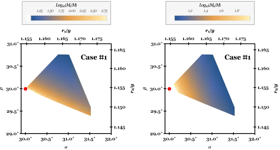
Figure 2. The allowed Case #1 regions that can produce central configurations in binary-star planetary systems. The plots demonstrate thatαandβare each limited to within a few degrees of 30◦. The colour contours indicate how much more restrictive this range is for different object masses: ForM2/M >102, bothαandβare confined to within a tenth of a degree of 30◦, whereas forM1/M >102,α andβ lie along the lower axis of the allowed region. Asteroids, pebbles or dust (withM1/M ≫1010, M2/M ≫1010) effectively lie at the critical point indicated by the red dot.
right-hand panels, this axis connects the other two objects. The difference between the middle and lower panels is the location of the centre-of-mass (“CoM”) of the systems. In all cases, the distance between either M object andM1 is
r1, and the distance between eitherM object andM2 isr2.
In the left-hand panels, the distance between theM objects is 2y, whereas in the right-hand panels the distance between both stars is 2y. ´Erdi & Czirj´ak (2016) designated Cases #1 and #2 as “convex”, Cases #3 and #4 as “the first concave case” and Cases #5 and #6 as “the second concave case”.
As demonstrated by ´Erdi & Czirj´ak (2016), if a config-uration is central, then one may obtain explicit analytical expressions for the mass ratios in terms of the geometrical anglesαandβ alone. These expressions differ by case, and in each instance there are restrictions onαandβ.
2.1 Cases #1-#2
2.1.1 Masses
I have found that one may obtain relatively compact explicit algebraic relations for central configurations by combining equations 36, 54-57, and 88 of ´Erdi & Czirj´ak (2016). Doing so gives, for Cases #1 and #2,
M1
M =
tanβ(tanα+ tanβ)2 8 cos3
β−1
4
(sinα+ cosαtanβ)3
−1 , (2)
M2
M =
tanα(tanα+ tanβ)2
8 cos3
α−1
4
(sinβ+ cosβtanα)3
−1 , (3)
subject to the restrictions
α = 30◦+ 2κ, (4)
β = 30◦+λκ, (5)
where
06κ615◦, (6)
−16λ62. (7)
2.1.2 Distances
The relative distances between bodies can be expressed in terms ofαandβonly, as readily seen on Fig. 1. I obtain
r1
y = secα, (8)
r2
y = secβ, (9)
r12
y = tanα+ tanβ, (10)
where r12 indicates the distance between masses M1 and
M2.
2.2 Cases #3-#6
2.2.1 Masses
4
Veras
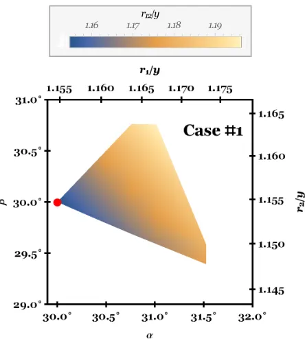
Figure 3. The distance between both stars in Case #1. Through-out the region which allows for central configurations to occur, both stars form a near-equilateral triangle shape (with side-length ratios differing by no more than five per cent) with each of the other objects.
M1
M =
tanβ(tanα−tanβ)2
1−8 cos3
β
4
(sinα−cosαtanβ)3−1 (11)
M2
M =
tanα(tanα−tanβ)2 1−8 cos3
α
4
(sinβ−cosβtanα)3+ 1 (12)
In Cases #3-#4, the anglesαandβare allowed to take on values according to
α = 45◦+κ, (13)
β = λκ, (14)
such that
06κ615◦, (15)
06λ62, (16)
whereas Cases #5-#6 instead require
α = 60◦+κ, (17)
β = 60◦+λ(15◦−κ), (18)
such that
06κ615◦, (19)
−26λ60. (20)
2.2.2 Distances
For all Cases #3-#6, the diagrams in Fig. 1 illustrate that
r1
y = secα, (21)
r2
y = secβ, (22)
r12
y = tanα−tanβ, (23)
wherer12 again indicates the distance between massesM1
andM2.
2.3 Overall
The last two sections explicitly illustrate the key insight of ´Erdi & Czirj´ak (2016) that the masses and distances be-tween four planar bodies, two of which have equal masses, and the other two defining an axis of symmetry, can be spec-ified entirely byαandβ. The conditions onαandβ, how-ever, require careful attention, as they are interdependent. Further, the transcendental nature of equations (2-3) and (11-12) demonstrates the difficulty or impossibility of ob-taining explicit formulae forα and β as a function of the masses.
The above results can be linked back to Λ from equation (1) through a transformation of equation 35 of ´
Erdi & Czirj´ak (2016), giving
Λ =−M1
r3 1
−M2
r3 2 −1 4 M y3 . (24)
Equation (24) may be expressed as the quantity Λy3
/M en-tirely in terms ofαandβ, helping to demonstrate that the values ofyandMeffectively represent scaling factors for all considered architectures.
3 LINK TO REAL PLANETARY SYSTEMS
Having established the computational method for this class of central configurations, I now show how they may be ap-plicable to planetary systems.
3.1 Mass cuts
To do so, I perform mass cuts, and then implicitly solve the equations from Section 2 to determine regions of phase space in which solutions exist. In all cases, I assume that each star is at least ten times the mass of the substellar objects, and that the two stellar masses are within a factor of ten of each other. These assumptions are realistic: the lowest-mass stars are a few tenths of a Solar mass, and the highest-mass planets are about an order of magnitude more highest-massive than Jupiter (∼0.01M⊙), roughly yielding a factor of ten
in extreme mass ratio. All stars which are known to host planetary systems have masses between 0.13M⊙−3.09M⊙ 1
– these stars include main sequence stars, giant branch stars, white dwarf stars and pulsars.
These assumptions also avoid some rare and ambigu-ous cases. For example, although a binary system consist-ing of a 100M⊙ star and 1M⊙ star might host a
plane-tary system, none have yet been observed, and would be
1
http://exoplanets.org/
c
Figure 4. Same as Fig. 2, but for Case #2. The allowed region for bothαandβis within a few degrees of 60◦, and most of the region is accessible only for large (super-Jupiter) planets. Smaller objects such as asteroids would be confined to the red dot.
extremely rare. Further, there is increasing evidence of a continuum of masses between planets and stars through brown dwarfs such as L dwarfs, T dwarfs and Y dwarfs (e.g. Skrzypek et al. 2016). Although the definition of “planet” has become ambiguous, the boundary between planet mass and brown dwarf mass still lies in a restricted range from about 0.010M⊙to 0.015M⊙(e.g. Spiegel et al. 2011).
My assumptions provide no lower bounds on masses: they can reach zero (but must not be negative). Depending on the level of accuracy sought, zero-mass objects could rep-resent a variety of objects, such as dust grains, pebbles or asteroids.
3.2 Results
Implementing these mass assumptions immediately yields one result: no solutions exist for Cases #3 or #5. This find-ing is indicated by red crosses in Fig. 1. Consequently, there exist no planar 4-body central configurations in binary-star planetary systems where the line of symmetry lies connects both stars and two equal-mass objects are “external” to both stars.
For the remaining cases, indicated by green check marks in Fig. 1, I created three plots per case to summarize the results. Each plot is a density plot as a function of the an-glesαandβand distance ratiosr1/yandr2/y. The angles
and distance ratios are quantities which are interchangeable (see equations 8-9 and 21-22). The density contours on the three plots respectively display a mass ratio involvingM1,
a mass ratio involving M2, and r12/y. The red dots
indi-cate extreme cases, where the mass ratios become either zero or infinite. White patches between the red dots and the differently-coloured regions indicate the gradient upon which this ratio takes a limiting value. The colour scale for
Figure 5. The distancer12between the substellar objects (M1 and M2), for Case #2. This value, combined with the allowed region forαandβ, indicates another near-rhombus-like configu-ration as in Case #1.
[image:6.612.307.533.361.610.2]6
Veras
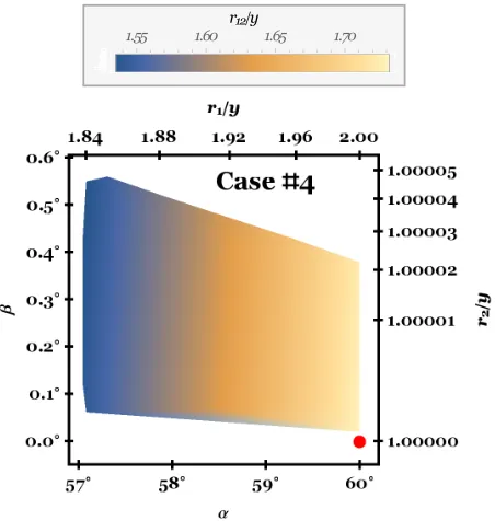
Figure 6. Same as Fig. 2, but for Case #4. Here, becauseα≈60◦andβ≈0◦, allowed geometries include a near-co-linear configuration of both stars plus one substellar body, with the other substellar body forming a near-equilateral triangle.
Figure 7. The distancer12between the substellar objects (M1 andM2), for Case #4.
3.2.1 Case #1 Results
Case #1 is the only unequal-mass star case that allows for central configurations. I present the results in Figs. 2-3.
One immediate striking observation is that the sim-ple a priori restriction of M1/M > 10, M2/M > 10 and
10−1 < M2/M1 < 10 reduces the relevant α phase space
range from 30◦(see equations 4 and 6) to about 1.5◦, and
theβphase space range of 45◦(see equations 5, 6 and 7) to
about 1.3◦. Another visually apparent feature is that mass
ratios of M1/M ∼ 100 hug the lower boundary of the
al-lowed region, whereas mass ratios ofM2/M ∼100 instead
approach the location of the red dot (α=β= 30◦), thereby
showcasing the asymmetry produced from unequal stellar masses.
Most of the allowed region is then restricted to 102
> M1/M >10 and 102> M2/M >10, meaning that
as-teroid, pebbles or other small objects are confined strongly to the location of the red dot. The formal limit of both
M1/M and M2/M at this value is infinity, meaning that
arbitrarily small objects can exist in central configurations there.
As emphasized by Fig. 3, the location of the red dot in-dicates when an equilateral triangle configuration is formed between both stars and either substellar object with mass
M. This architecture then resembles a rhombus with two in-ternal angles of 120◦ and the other two with 60◦. The stars
would be at the vertices associated with the 120◦ angles. Effectively, this configuration is a doubled-up version of the classic 3-body Lagrangian triangle, at least in terms of ge-ometry. In binary-star planetary systems, deviations from this rhombus configuration extend only a few degrees inα
andβ, at most.
3.2.2 Case #2 Results
I present the Case #2 results in Figs. 4-5. In Case #2, the stellar masses are equal and do not define the axis of sym-metry. Nevertheless, the inequality of the masses of the sub-stellar objects still produce a noticeable difference in the locations of the lightly-coloured regions between both pan-els of Fig. 4. Just as for Case #1, the restriction of phase space due to the assumption of a planetary system is simi-larly stark: down to a range of about 0.9◦in bothαandβ.
Only super-Jupiter mass planets could exist in central
con-c
[image:7.612.44.270.350.588.2]figurations more than a few tenths of a degree away from 60◦for either angle.
The values of the mass ratios M/M1 and M/M2 both
approach infinity as the red dot (α=β= 60◦) is itself ap-proached, indicating thatM1 →0 andM2 →0 is allowed.
The red dot corresponds to a rhombus similar to that pro-duced from the critical red dot location in Case #1, except rotated by 90◦ and in the limit that both stars have equal
masses.
3.2.3 Case #4 Results
Case #4 is a fundamentally different geometry than Cases #1 and #2. This difference is reflected in how the allowed phase space inαandβis restricted (Figs. 6-7). The value of
αis restricted to 57◦−60◦whileβis restricted to 0.0◦−0.57◦.
Effectively, these restrictions place M2 nearly in-between
both stars such that M1 is in a near-equilateral triangle
configuration with the three near-co-linear bodies. At the critical point (α= 60◦,β= 0◦), the values ofM
1 andM2
approach zero. This combination of a co-linear configura-tion with an equilateral triangle configuraconfigura-tion represents a superposition of two three-body central configurations.
3.2.4 Case #6 Results
Case #6 is geometrically equivalent to Case #4 except for the location of the centre of mass. This difference creates a significant change in the allowed α-β phase-space region (Figs. 8-9), with a range that extends to almost 10◦inβand
7◦ in α. At the critical point α=β = 60◦, an equilateral
triangle with one vertex that is “doubled up” with bothM1
and M2 (which would coincide) is formed. The kink which
appears in the diagonal on each plot indicates the point at which theM = 10M1 andM = 10M2 mass cuts were made.
4 DISCUSSION
This study demonstrates that central configurations in binary-star planetary systems may exist, and quantifies the extent of the existence region. Whether objects residing in the immediate vicinity of these configurations are long-term stable and have plausible dynamical origins are different questions.
A proper stability analysis of planar four-body central configurations with two equal masses and an axis of symme-try connecting the unequal masses has not yet been carried out, and could represent a significant undertaking. The re-sults here might help focus that effort by quantifying the variations in geometries and mass that result from the most basic planetary system-based restrictions.
Regarding the likelihood of a planetary system forming or settling into one of the central configurations discussed here, the chances probably increase as the substellar masses decrease. All these central configurations include objects which are nearly co-orbital or nearly co-linear. No planets as massive as Jupiter have yet to be found in such architectures. The largest known co-orbital objects in the solar system are Janus (1×10¹⁸
kg) and Epimetheus (5×10¹⁷
kg), and in extrasolar systems is a minor planet with its disrupted frag-ments orbiting white dwarf WD 1145+017; the mass of this
Figure 9. The distancer12between the substellar objects (M1 andM2), for Case #6. Unlike for Cases #1, #2 and #4, hereM1 andM2would coincide at the critical point.
minor planet is likely to be about 1020
kg, a tenth of the mass of Ceres (Gurri et al. 2016; Rappaport et al. 2016). Multi-ple co-orbital masses above 1023
kg are roughly assumed to become unstable at the 20 per cent level (Veras et al. 2016). Three or more co-linear planetary objects are not known to exist in stable configurations.
The fact that the majority of planets in the solar sys-tem host at least one Trojan asteroid might indicate that capture into that central configuration is common. If so, the extended Trojan-analogue rhombus configurations from Cases #1 and #2 might also be easily populated by aster-oids or smaller bodies such as pebbles or dust or gas. In fact, remnant protoplanetary disc features might reside in the locations indicated by the red dots on Figs. 2-5.
Finally, I emphasize that these configurations are fully scalable with y and M. The binary stars could have wide separations of 104
au or close separations of 10−2
au. Such close separations are unlikely to host objects in central con-figurations because any bodies so close to those stars would either be drawn in and destroyed due to tides, or blown away by winds. For particularly wide separations, com-parable to where stellar flybys or planet-planet scattering might deposit planets or planetary debris into an exosystem (Perets & Kouwenhoven 2012; Varvoglis et al. 2012), cap-ture into a central configuration is a distinct possibility.
5 SUMMARY
Central configurations are complete analytic solutions to the
8
Veras
Figure 8. Same as Fig. 2, but for Case #6. Here,αexceeds 60◦andβis short of 60◦. When the two angles coincide, then an equilateral triangle would be formed with one star at each vertex and both substellar masses at the other.
point masses without the need for numerical integration. I have quantified where in phase space do central configura-tions exist for coplanar four-body binary-star exoplanetary systems containing one axis of symmetry, two stars whose masses are within a factor of ten of each other, and two sub-stellar bodies whose masses are no greater than a tenth of either stellar mass.
I found that these basic mass restrictions – which sat-isfy virtually every known planetary system – significantly restrict the geometries in which central configurations may occur to within a few degrees of two architectures and ten degrees of a third. These architectures are all extensions of the well-known observed Sun-Jupiter-Trojan configuration, and occur in the limit of zero-mass substellar masses. The first architecture (Cases #1 and #2) is a rhombus with both stars at opposite ends whose associated internal angles are 120◦. The second (Case #4) features a co-linear
configura-tion of two equal-mass stars plus one substellar body, with the second substellar body forming an equilateral triangle. The third (Case #6) is an equilateral triangle configuration with the two substellar masses at one vertex.
As the mass of substellar bodies (which may be e.g. planets, asteroids, pebbles, dust) increases, the deviation from these limiting architectures must increase in order to achieve the central configuration. These mass restrictions also importantly exclude central configurations for the ar-chitectures of Cases #3 and #5. Binary stars need not be of equal mass nor classed as close nor wide in order to achieve central configurations.
ACKNOWLEDGEMENTS
I thank the referee for their expert comments, particularly about Case #6. I have received funding from the Euro-pean Research Council under the EuroEuro-pean Union’s Sev-enth Framework Programme (BP/2007-2013)/ARC Grant Agreement n. 320964 (WDTracer).
REFERENCES
Chiang, E. I., & Lithwick, Y. 2005, ApJ, 628, 520 Davies, M. B., Adams, F. C., Armitage, P., et al. 2014,
Protostars and Planets VI, 787 ´
Erdi, B., & Czirj´ak, Z. 2016, Celestial Mechanics and Dy-namical Astronomy, 125, 33
Euler, L. 1767, De motu rectilineo trium corporum se mu-tuo attrahentium, Novi Comm. Acad. Sci. Imp. Petrop. 11:144-151.
Gurri, P. Veras, D., G¨ansicke, B. T. 2016, Submitted to MNRAS
Hamilton, D. P. 2016, Nature, 533, 187
Hardy, A., Schreiber, M. R., Parsons, S. G., et al. 2016, MNRAS, 459, 4518
Kiefer, F., Lecavelier des Etangs, A., Boissier, J., et al. 2014, Nature, 514, 462
Lagrange, J. L. 1772, Essai sur le problme des trois corps, Oeuvres, vol. 6.
Llibre, J., Moeckel, R., Sim, C. 2015, Central Configura-tions, Periodic Orbits, and Hamiltonian Systems. Springer Basel.
Lykawka, P. S., Horner, J., Jones, B. W., & Mukai, T. 2009, MNRAS, 398, 1715
c
Marchal, C., & Bozis, G. 1982, Celestial Mechanics, 26, 311 Moeckel, R. 1990, Mathematische Zeitschrift, 205, 499-517. Morbidelli, A., Levison, H. F., Tsiganis, K., & Gomes, R.
2005, Nature, 435, 462
Perets, H. B., & Kouwenhoven, M. B. N. 2012, ApJ, 750, 83
Rappaport, S., Gary, B. L., Kaye, T., et al. 2016, MNRAS, 458, 3904
Rapson, V. A., Sargent, B., Sacco, G. G., et al. 2015, ApJ, 810, 62
Skrzypek, N., Warren, S. J., & Faherty, J. K. 2016, A&A, 589, A49
Spiegel, D. S., Burrows, A., & Milsom, J. A. 2011, ApJ, 727, 57
Vanderburg, A., Johnson, J. A., Rappaport, S., et al. 2015, Nature, 526, 546
Varvoglis, H., Sgardeli, V., & Tsiganis, K. 2012, Celestial Mechanics and Dynamical Astronomy, 113, 387