warwick.ac.uk/lib-publications
A Thesis Submitted for the Degree of PhD at the University of Warwick
Permanent WRAP URL:
http://wrap.warwick.ac.uk/80139
Copyright and reuse:
This thesis is made available online and is protected by original copyright.
Please scroll down to view the document itself.
Please refer to the repository record for this item for information to help you to cite it.
Our policy information is available from the repository home page.
M A
E
G
NS I
T A T MOLEM
U N
IV
ER
SITAS WARWICEN
SIS
Limit Structures and Property Testing
by
Tereza Klimoˇ
sov´
a
Thesis
Submitted to the University of Warwick
for the degree of
Doctor of Philosophy
Mathematics Institute
Contents
List of Figures iii
List of Tables iv
Acknowledgments v
Declarations vi
Abstract vii
Notation and Preliminaries 1
Chapter 1 Introduction 3
1.1 Limit objects and finite forcibility . . . 4
1.1.1 Limits of permutations . . . 4
1.1.2 Limits of dense graphs . . . 6
1.1.3 Finite forcibility . . . 6
1.1.4 Statements of our results . . . 7
1.2 Property and parameter testing . . . 12
Chapter 2 Finitely forcible graphons and permutons 17 2.1 Cumulative distribution function . . . 17
2.2 Permutons with finite structure . . . 19
2.3 Permutons with infinite structure . . . 21
2.4 Graphons with infinite structure . . . 30
2.4.1 Union of complete graphs . . . 30
2.4.2 Union of random graphs . . . 32
Chapter 3 Infinitely dimensional finitely forcible graphon 34 3.1 Finite forcibility . . . 34
3.2 The hypercubical graphon . . . 38
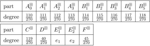
3.3 Constraints . . . 45
3.4.1 Forcing [0,1]×C—triangular constraints . . . 56
3.4.2 Forcing the structure on A1×A1 . . . 57
3.4.3 Forcing the remaining diagonal checker subgraphons . . . 57
3.4.4 Forcing the structure of A0×A1 . . . 58
3.4.5 Partitioning W into levels . . . 58
3.4.6 Stair constraints . . . 59
3.4.7 Coordinate constraints . . . 60
3.4.8 Initial coordinate constraint . . . 60
3.4.9 Distribution constraints . . . 60
3.4.10 Product constraints . . . 61
3.4.11 Projection constraints . . . 62
3.4.12 Infinite constraints . . . 65
3.4.13 Structure involving the partsE1, E2 and F . . . 66
Chapter 4 Erd˝os-Lov´asz-Spencer theorem for permutations 68 4.1 Permutation densities . . . 68
4.2 Properties of the sets Tq and Tq mon . . . 72
Chapter 5 Non-forcible approximable parameter 76 Chapter 6 Property testing algorithms for permutations 79 6.1 Branchings . . . 79
6.2 Decompositions . . . 81
6.3 Testing . . . 85
List of Figures
1.1 The limits of permutation sequences. . . 5
1.2 The graphons associated with permutons. . . 8
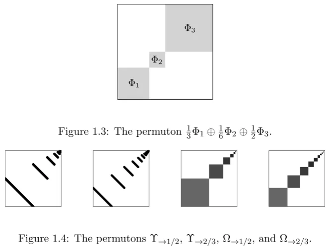
1.3 The permuton 13Φ1⊕16Φ2⊕ 12Φ3. . . 9
1.4 The permutons Υ→1/2, Υ→2/3, Ω→1/2, and Ω→2/3. . . 9
2.1 The permuton ΦM. . . 21
2.2 Notation used in equalities (2.20) and (2.21). . . 28
3.1 The hypercubical graphon. . . 39
3.2 The diagonal checker functionκ. . . 40
3.3 Constraint forcing zero edge density. . . 46
3.4 The degree unifying constraints. . . 47
3.5 The degree unifying constraints forD. . . 47
3.6 The degree distinguishing constraints for F×C. . . 49
3.7 The triangular constraints. . . 49
3.8 The main diagonal checker constraints. . . 49
3.9 The complete bipartition constraints. . . 49
3.10 The auxiliary diagonal checker constraints. . . 50
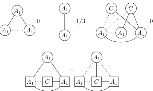
3.11 The first level constraints. . . 50
3.12 The stair constraints. . . 50
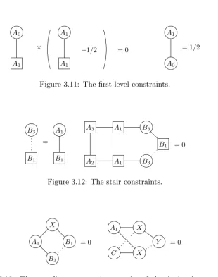
3.13 The coordinate constraints . . . 50
3.14 The distribution constraints. . . 51
3.15 The initial coordinate constraint. . . 51
3.16 The product constraints forB4. . . 52
3.17 The product constraints forB5. . . 52
3.18 The first four projection constraints. . . 53
3.19 The last two projection constraints. . . 54
3.20 Infinite constraints. . . 54
3.21 Density expressions specifying levels of vertices. . . 59
List of Tables
Acknowledgments
I am very grateful to many people for their both scientific and non-scientific
help, support and inspiration during my studies.
First of all, my big thanks go to Dan Kr´al’ for being a very helpful
and patient advisor. I would also like to thank all my coauthors for enjoyable
collaboration.
I am grateful to my colleagues and fellow students, both from the
Uni-versity of Warwick and from the Charles UniUni-versity, where I spent the first year
of my PhD studies, for creating an inspiring and friendly atmosphere. I would
also like to thank to attentive audience on my talks for their questions and for
making me feel that my research makes sense.
My special thanks go to Tom´aˇs Pokorn´y for resuscitating my laptop.
Last, but not least, I would like to thank my family and my boyfriend for their
Declarations
The thesis contains results which were obtained together with collaborators and
published as follows.
The results from Chapter 2 were obtained together with R. Glebov,
A. Grzesik and D. Kr´al’. The corresponding paper R. Glebov, A. Grzesik,
T. Klimoˇsov´a, and D. Kr´al’: Finitely forcible graphons and permutons was
published in Journal of Combinatorial Theory, Series B 110 (2015), 112–135
and is also available as arXiv:1307.2444. The results from this chapter are also
a part of the PhD thesis of A. Grzesik.
The results from Chapter 3 were obtained together with R. Glebov and
D. Kr´al’. The corresponding paper R. Glebov, T. Klimoˇsov´a, and D. Kr´al’:
Infinite dimensional finitely forcible graphonis available as arXiv:1404.2743 and
has been submitted to a journal.
The results from Chapters 4 and 5 were obtained together with R.
Gle-bov, C. Hoppen, Y. Kohayakawa, D. Kr´al’, and H. Liu. The corresponding
paper R. Glebov, C. Hoppen, T. Klimoˇsov´a, Y. Kohayakawa, D. Kr´al’, and
H. Liu: Large permutations and parameter testingis available as arXiv:1412.5622
and has been submitted to a journal.
The results from Chapter 6 were obtained together with D. Kr´al’. The
corresponding paperT. Klimoˇsov´a and D. Kr´al’: Hereditary properties of
per-mutations are strongly testable was published in Proceedings of SODA 2014,
SIAM, Philadelphia, PA, 1164–1173 and is also available as arXiv:1208.2624.
With the exception of Chapter 2, as indicated above, none of the results
appeared in any other thesis.
All the collaborators have agreed with the inclusion of our joint work
Abstract
In the thesis, we study properties of large combinatorial objects. We
analyze these objects from two different points of view.
The first aspect is analytic—we study properties of limit objects of
com-binatorial structures. We investigate when graphons (limits of graphs) and
per-mutons (limits of permutations) are finitely forcible, i.e., when they are uniquely
determined by finitely many densities of their substructures. We give examples
of families of permutons that are finitely forcible but the associated graphons
are not and we disprove a conjecture of Lov´asz and Szegedy on the dimension
of the space of typical vertices of a finitely forcible graphon. In particular, we
show that there exists a finitely forcible graphonW such that the topological
spacesT(W) andT(W) have infinite Lebesgue covering dimension.
We also study the dependence between densities of substructures. We
prove a permutation analogue of the classical theorem of Erd˝os, Lov´asz and
Spencer on the densities of connected subgraphs in large graphs.
The second aspect of large combinatorial objects we concentrate on
is algorithmic—we study property testing and parameter testing. We show
that there exists a bounded testable permutation parameter that is not finitely
forcible and that every hereditary permutation property is testable (in
con-stant time) with respect to the Kendall’s tau distance, resolving a conjecture
Notation and Preliminaries
In this section we survey basic notation and terminology for graphs and per-mutations that is used throughout the thesis.
We useN∗ forN∪ {∞} and [n] for {1, . . . , n}. We also set [∞] =N. If
aandb are integers, thenamodbis equal to the integer x∈[b] with the same remainder asaafter division byb. AnintervalI in [n] is a set of integers of the form {k|a≤k≤b} for some a, b∈[n]. If a < b and I 6= [n] we say that I is proper.
A collection of setsS ={S1, . . . , S`} is apartition of a set S of order`
ifS =∪i∈[`]Si and Si∩Sj =∅ for every i6=j, i, j∈ [`]. We denote the order
of a partitionS by|S|.
We useλk for thek-dimensional Lebesgue measure andυkfor its
restric-tion to theσ-algebra of Borel sets. (In different parts of the thesis, we need to specifically consider either one or the other.) In other words, υk is a uniform
measure on theσ-algebra of Borel sets. We omit the subscript if the dimension is clear from the context.
For a non-trivial convex polygon A ⊆ [0,1]2, i.e., a convex polygon different from a point (but it can be a segment), we define ΥAto be the unique
probability measure on theσ-algebra of Borel sets of [0,1]2with supportAand mass uniformly distributed inside A. That is, for every Borel set S ⊆ [0,1]2, ΥA(S) =υ2(A∩S)/υ2(A) forAwithυ2(A)>0, and ΥA(S) =υ1(A∩S)/υ1(A) ifυ2(A) = 0, in which caseAmust be a segment andυ1 is the uniform measure on the line containing the segment A. In particular, Υ[0,1]2 coincides with υ2 on [0,1]2. We set Υ = Υ
[0,1]2 to simplify the notation. A graph is a pair (V, E) where E ⊆ V2
. The elements of V are called vertices and the elements ofE are called edges. Theorder of a graphG is the number of its vertices and it is denoted by|G|.
If G and G0 are graphs, then G∪G0 is the disjoint union of G and G0 and G+G0 is the graph obtained fromG∪G0 by adding all edges betweenG
Thedensityt(H, G) of a graphHin a graphGis the probability that|H| distinct vertices ofGchosen uniformly at random induce a subgraph isomorphic toH. If|H|>|G|, we sett(H, G) = 0.
A permutation of order n is a bijective mapping from [n] to [n]. The order of a permutation π is also denoted by |π|. We will call a permutation non-trivial if it has order greater than 1. The set of all permutations is denoted bySand the set all permutations of ordernbySn. In what follows, we identify
a sequence ofndistinct integersa1. . . anbetween 1 andnwith a permutationπ
by settingπ(i) =ai. For example, the identity permutation of order 4 is denoted
by 1234. Aninversion in a permutation σ is a pair (i, j), i, j∈[|σ|], such that i < j and σ(i)> σ(j).
Letσ be a permutation of ordernandX={x1, . . . , xk} ⊆[n] such that
x1 <· · ·< xk. Asubpermutation induced byXinσ denoted byπ=σ X is a
permutation of orderksuch thatπ(j)< π(j0) if and only ifσ(xj)< σ(xj0). For example, the subpermutation of 7126354 induced by 3,4,6 is 132. We say that σ containsπ as a subpermutation if there exists X⊆[n] such that π=σX. In some literature, subpermutations are referred to as patterns. However, we follow the terminology from previous papers related to testing permutation properties and to permutation limits, which also makes the terminology closer to the case of graphs.
Chapter 1
Introduction
In the thesis, we study properties of large combinatorial objects. We analyze these objects from two different points of view.
The first aspect is analytic—we study properties of limit objects of com-binatorial structures. We investigate when graphons (limits of graphs) and per-mutons (limits of permutations) are finitely forcible, i.e., when they are uniquely determined by finitely many densities of their substructures. In Chapter 2, we give examples of families of permutons that are finitely forcible but the associ-ated graphons are not.
Our efforts in studying finite forcibility culminate in Chapter 3, where we disprove a conjecture of Lov´asz and Szegedy on the dimension of the space of typical vertices of a finitely forcible graphon. In particular, we show that there exists a finitely forcible graphonW such that the topological spacesT(W) and T(W) have infinite Lebesgue covering dimension.
In Chapter 4, we study the dependence between densities of substruc-tures. We prove a permutation analogue of the classical theorem of Erd˝os, Lov´asz and Spencer on the densities of connected subgraphs in large graphs.
In Chapter 6, we show that every hereditary permutation property is testable (in constant time) with respect to the Kendall’s tau distance, resolving a conjecture of Kohayakawa [58].
In the remainder of this chapter, we survey definitions and put the results contained in the thesis into the context of previous work.
1.1
Limit objects and finite forcibility
Research on analytic objects associated with convergent series of combinatorial objects was initiated by the theory of limits of dense graphs [20–22,66], followed by limits of sparse graphs [18, 34], permutations [52, 53], partial orders [56] and others. This theory provides an analytic view of many standard concepts, e.g., the regularity method [68], and led to results in many areas of mathematics and computer science, in particular in extremal combinatorics [9–12, 49–51, 59, 60, 71, 72, 74–76] and property testing [54, 69].
In the thesis, we focus on limits of dense graphs, which are called graphons and limits of permutations, which are called permutons. We start our exposition with the slightly simpler notion of permutation limits.
1.1.1 Limits of permutations
The theory of permutation limits was initiated by Hoppen, Kohayakawa, Mor-eira, R´ath and Sampaio in [52, 53]. Here, we follow the analytic view on the limit as used in [61], which also appeared in an earlier work of Presutti and Stromquist [73].
An infinite sequence (πi)i∈Nof permutations with|πi| → ∞isconvergent if the sequence (t(σ, πi))i∈N converges for every permutation σ. With every
convergent sequence of permutations, one can associate the following analytic object: apermutonis a probability measure Φ on theσ-algebraAof Borel sets of the unit square [0,1]2such that Φ hasuniform marginals, i.e., Φ([α, β]×[0,1]) = Φ([0,1]×[α, β]) = β −α for every 0 ≤ α ≤ β ≤ 1. We denote the set of all permutons byP.
We now describe the relation between convergent sequences of permuta-tions and permutons. Let Φ be a permuton. For an integern, let (x1, y1), . . . , (xn, yn) be points in [0,1]2 sampled independently according to the
distri-bution Φ. Because Φ has uniform marginals, the x-coordinates of all these points are mutually different with probability one. The same holds for the y-coordinates. Assume that this is indeed the case. One can then define a permutationπ of ordernbased on thenpoints (x1, y1), . . . ,(xn, yn) as follows:
Figure 1.1: The limits of sequences π1
i
i∈N, π 2
i
i∈N, π 3
i
i∈Nand π 4
i
i∈N.
unique bijective mapping from [n] to [n] satisfying π(j) < π(j0) if and only if yij < yij0. We say that a permutationπof ordernobtained in the just described way is a Φ-random permutation of ordern. A uniformly random permutation is a Υ-random permutation (note that Υ = Υ[0,1]2 is a permuton), i.e., each permutation of ordernis chosen with probability (n!)−1.
If Φ is a permuton andσ is a permutation of ordern, thent(σ,Φ) is the probability that a Φ-random permutation of ordernisσ. We now recall the core results from [52, 53]. For every convergent sequence (πi)i∈N of permutations, there exists a unique permuton Φ such that t(σ,Φ) = limi→∞t(σ, πi) for every
permutationσ. This permuton is thelimitof the sequence (πi)i∈N. On the other
hand, let Φ be a permuton and (πi)i∈N a sequence such that πi is a Φ-random permutation of order i. With probability one, this sequence is convergent and its limit is Φ.
We now give four examples of the notions we have just defined (the corresponding permutons are depicted in Figure 1.1). Let us consider a sequence
π1
i
i∈N such that π
1
i is the identity permutation of order i, i.e., πi1(k) = k for
k∈[i]. This sequence is convergent and its limit is the the permuton I = ΥA
whereA={(x, x), x∈[0,1]}. Similarly, the limit of a sequence π2
i
i∈N, where
π2
i is the permutation of order i defined as π2i(k) = i+ 1−k for k ∈ [i], is
the permuton Ω = ΥB where B = {(x,1−x), x∈[0,1]}. A little bit more
complicated example is the following: the sequence π3
i
i∈N, where πi3 is the
permutation of order 2idefined as
π3i(k) =
2k−1 ifk∈[i],
2(k−i) otherwise
is convergent and the limit of the sequence is the measure 1 2ΥC +
1
2ΥD, where C={(x/2, x), x∈[0,1]}and D={((x+ 1)/2, x), x∈[0,1]}. Next, consider a sequence (π4
i)i∈N such that πi4 is a uniformly random permutation of order i.
1.1.2 Limits of dense graphs
The other limit structures we consider are limits of dense graphs. We now survey basic results related to the theory of dense graph limits as developed in [20–22, 66]. A sequence of graphs (Gi)i∈N with|G| → ∞ isconvergent if the sequence (t(H, Gi))i∈N converges for every H. The associated limit object is
called agraphon: it is a symmetricλ-measurable function from [0,1]2 to [0,1]. Here, symmetric stands for the property that W(x, y) = W(y, x) for every x, y∈[0,1]. If W is a graphon, then aW-random graph of orderk is obtained by sampling k random points x1, . . . , xk ∈ [0,1] uniformly and independently
and joining thei-th and the j-th vertex by an edge with probability W(xi, xj).
As in the case of permutations, we write t(H, W) for the probability that a W-random graph of order |H|is isomorphic toH.
The densities of graphs in a graphon W can be expressed as integrals. IfW is a graphon andHis a graph of order kwith verticesv1, . . . , vk and edge
setE, then
t(H, W) = k!
|Aut(H)|
Z
[0,1]k
Y
vivj∈E
W(xi, xj) Y
vivj6∈E
(1−W(xi, xj))dx1. . .dxk
where Aut(H) is the automorphism group of H.
For every convergent sequence (Gi)i∈N of graphs, there exists a graphon
W such that t(H, W) = limi→∞t(H, Gi) for every graph H [66]. We call such
a graphon W a limit of (Gi)i∈N. On the other hand, for a graphon W, the sequence (Gi)i∈N where Gi is a W-random graph of order i is convergent with
probability one and its limit isW with probability one.
Unlike in the case of permutations, the limit of a convergent sequence of graphs is not unique. For a graphonW and a measure preserving transformation ϕ: [0,1]→[0,1], letWϕ=W(ϕ(x), ϕ(y)). Then, ifW is a limit of (G
i)i∈N,Wϕ is also a limit of (Gi)i∈N. Let us introduce the following definition of equivalence
of graphons: two graphons W and W0 are weakly isomorphic if t(H, W) =
t(H, W0) for every graphH. The following equivalent characterization of weak isomorphism was given in [19].
Theorem 1. Two graphonsU andW are weakly isomorphic if and only if there exist measure preserving maps ϕ, ψ: [0,1]→[0,1] such that Uϕ =Wψ almost
everywhere.
1.1.3 Finite forcibility
such that every graphon W0 satisfying t(H, W) = t(H, W0) for every H ∈ H
is weakly isomorphic toW. Similarly, a permuton Φ isfinitely forcible if there exists a finite set S of permutations such that every permuton Φ0 satisfying
t(σ,Φ) =t(σ,Φ0) for everyσ ∈S is equal to Φ. In other words, a graphon or a permuton is finitely forcible, if it can be uniquely determined (up to weak iso-morphism in the case of graphons) by finitely many densities of substructures. The question whether a graphon or a permuton is finitely forcible is particularly interesting from the point of view of extremal combinatorics, since every finitely forcible object corresponds to the unique solution of some ex-tremal problem. Problems of this kind are also related to quasirandomness and they were studied well before the theory of limits of combinatorial objects emerged. For example, the results on quasirandom graphs from the work of Chung, Graham and Wilson [24], R¨odl [78] and Thomason [84,85] imply that the homomorphic densities ofK2 and C4 guarantee that densities of all subgraphs behave as in the random graphGn,1/2. In the language of graphons, this result asserts that the graphon identically equal to 1/2 is finitely forcible by densities of 4-vertex subgraphs. A similar result for permutations, which was originally raised as a question by Graham, was proven by Kr´al’ and Pikhurko [61] who exploited the analytic view on permutation limits to show that the random permuton is finitely forced by densities of permutations of order 4.
The results on graphs were generalized for stepwise graphons in [64]. Another example of a finitely forcible graphon is due to Diaconis, Homes, and Janson [32]. Their result is equivalent to the statement that the half-graphon W4(x, y) defined asW4(x, y) = 1 ifx+y≥1, andW4 = 0, otherwise, is finitely
forcible. These results were further extended by Lov´asz and Szegedy [65] who also gave several conditions when a graphon is not finitely forcible. In Chapter 2, we provide a generalization of these results in the realm of permutons.
1.1.4 Statements of our results
In Chapter 2, we focus on the interplay between finite forcibility of permutons and graphons. In [64], Lov´asz and S´os proved a result for more complex quasirandom graphs, which can be restated in the language of graphons as a statement that any stepwise graphon1is finitely forcible. We prove the following analogue of this result for permutons.
1
A graphonW isstepwiseif there exists a partition of [0,1] into finitely many measurable
Figure 1.2: The graphons associated with the first three permutons depicted in Figure 1.1, where the point (0,0) is in the bottom left corner.
Theorem 2. If Φ is a permuton satisfying Φ = Pi∈[k]αiΥAi for some
non-negative reals α1, . . . , αk and some non-trivial polygons A1, . . . , Ak ⊆ [0,1]2,
thenΦ is finitely forcible.
A permutationπ of orderkcan be associated with a graph Gπ of order
kas follows. The vertices of Gπ are the integers between 1 andk and ij is an
edge ofGif and only if either i < j and π(i)> π(j), or i > j and π(i)< π(j), i.e., iand j form an inversion. If (πi)i∈N is a convergent sequence of permuta-tions, then the sequence of graphs (Gπi)i∈Nis also convergent. Moreover, if two convergent sequences of permutations have the same limit, then the graphons associated with the two corresponding (convergent) sequences of graphs are weakly isomorphic. In this way, we may associate each permuton Φ with a graphon WΦ, which is unique up to a weak isomorphism (see Figure 1.2 for examples). We will provide examples of classes of permutons that are finitely forcible, while the associated graphons are not.
For k ∈ N∗, let (W)i∈[k] be a sequence of graphons and (pi)i∈[k] ∈ Rk+ be a sequence of reals such that Pi∈[k]pi = 1. We define a direct sum of graphonsWi with weights pi denoted by W =Li∈[k]piWi as follows.
W(x, y) =
Wi(ϕi(x), ϕi(y)) if x, y∈Ji for somei∈[k], and
0 otherwise,
where
Ji =
i−1
X
j=1 pj,
i X
j=1 pj
and
ϕi(x) =
x−Pij−=11pj pi
for everyi∈[k].
We now define the direct sum of permutons with weights in an analogous way. Fork∈N∗, a sequence of permutons (Φi)i∈[k]and (pi)i∈[k]∈Rk+such that
P
i∈[k]pi = 1, the direct sum of permutons Φi with weights pi is denoted by
Φ1
Φ2
Φ3
[image:18.595.125.457.68.317.2]Figure 1.3: The permuton 13Φ1⊕16Φ2⊕ 12Φ3.
Figure 1.4: The permutons Υ→1/2, Υ→2/3, Ω→1/2, and Ω→2/3.
Φ(S) = X
i∈[k]
piΦi(θi(S∩Ci))
for every Borel set S, where Ci = Ji×Ji and θi is a map from Ci to [0,1]2
defined as θi((x, y)) = (ϕi(x), ϕi(y)) for every i ∈ [k]. See Figure 1.3 for an
example.
For a graphonW and α∈(0,1), we define a graphon
W→α =
∞
M
i=1
(1−α)αi−1W.
Similarly, for a permuton Φ andα∈(0,1), we define
Φ→α =
∞
M
i=1
(1−α)αi−1Φ.
Later, we prove finite forcibility of permutons Ω→α and Υ→α. (Recall
that Ω denotes the unique permuton with support consisting of the segment between (0,1) and (1,0).) Examples of these permutons can be found in Fig-ure 1.4.
Theorem 3. For every α ∈ (0,1), the permutons Ω→α and Υ→α are finitely
Next, we turn our attention to graphons with similar recursive structure. We show that graphons of this kind are not finitely forcible unless they are equal to zero almost everywhere.
Theorem 4. For every α∈(0,1) and every graphon W, if the graphon W→α
is finitely forcible, thenW is equal to zero almost everywhere.
Consequently,W→α is finitely forcible only ifW zero almost everywhere.
Observe that WΦ→α and (WΦ)→α are weakly isomorphic. It follows that the graphonsWΩ→α and WΥ→α associated with the permutons Ω→α and Υ→α are weakly isomorphic to (WΩ)→α and (WΥ)→α, respectively and therefore not
finitely forcible.
In Chapter 3, we study a relation between finite forcibility and properties of typical vertices of a graphon. Every graphon can be assigned a topological space associated with its typical vertices as follows [67]. For a graphonW and x∈[0,1], we define a function
fxW(y) =W(x, y).
Since almost every functionfW
x belongs toL1([0,1]), the graphonW naturally
defines a probability measure µon L1([0,1]). Let T(W) be the set formed by the functionsf ∈L1([0,1]) such that every neighborhood off inL1([0,1]) has positive measure with respect toµ. The setT(W) with the topology inherited from L1([0,1]) is called the space of typical vertices of W. The vertices x of W with fW
x ∈T(W) are called typical vertices of a graphon W. A coarser
topology on T(W) can be defined using the similarity distance dW between
f, g∈L1([0,1]) defined as
dW(f, g) = Z
[0,1]
Z
[0,1]
W(x, y)(f(y)−g(y))dy
dx.
The space with this topology is denoted byT(W). The topological spaceT(W) is always compact [63, Chapter 13] and its structure is related to weak regular partitions ofW [68].
UnlikeT(W), T(W) does not need to be compact even if W is finitely forcible [42]. Lov´asz and Szegedy [65, Conjecture 10] led by examples of known finitely forcible graphons proposed the following:
Conjecture 1. If W is a finitely forcible graphon, then T(W) is finite
They said that they intentionally do not specify which notion of dimen-sion is meant here—a result concerning any variant would be interesting. The Rademacher graphon WR constructed in [42] is finitely forcible and the space
T(WR) has infinite Minkowski dimension but its Lebesgue dimension is one and
T(WR) has both Minkowski and Lebesgue dimension one.
We construct a graphonW, which we call ahypercubical graphon, such that W is finitely forcible and both T(W) and T(W) contain subspaces homeomorphic to [0,1]N.
Theorem 5. The hypercubical graphon W is finitely forcible and the
topolog-ical spacesT(W) and T(W) contain subspaces homeomorphic to [0,1]N.
The proof of Theorem 5 extends the methods from [42] and [70]. In particular, Norine [70] constructed finitely forcible graphons with the space of typical vertices of arbitrarily large (but finite) Lebesgue dimension. In his construction, bothT(W) andT(W) contain a subspace homeomorphic to [0,1]d.
We show how the techniques from [42] and [70] can be refined to force a subspace homeomorphic to [0,1]N, which turned out to be quite technically challenging. In Chapter 4, we use limit objects of permutations to prove a permuta-tion analogue of a classical result of Erd˝os, Lov´asz and Spencer about subgraph densities in a graph. In the case of graphs, Erd˝os, Lov´asz and Spencer [35] considered three notions of substructure densities: the subgraph density, the induced subgraph density and the homomorphism density. They showed that these types of densities are strongly related and that the densities of connected graphs are independent. The result has a natural formulation in the language of graphons: the body of possible densities of anykconnected graphs in graphons, which is a subset of [0,1]k, has a non-empty interior (in particular, it is full
di-mensional).
1.2
Property and parameter testing
In Chapters 5 and 6 we focus on algorithmic aspects of large combinatorial structures, in particular on property and parameter testing.
Aproperty testeris an algorithm that decides whether a large input has the considered property by querying only a small sample of it. Since the tester is presented only with a part of the input, it is necessary to allow an error based on the robustness of the tested property. Following [43, 45, 48, 79–81], we say that a property P of a class of structures (e.g., functions, graphs) is testable if for every ε >0, there exists a randomized algorithm (a tester) A such that the number of queries made byAis bounded by a function ofεindependent of the input and such that if the input has the property P, then A accepts with probability at least 1−ε, and if the input is ε-far fromP, thenA rejects with probability at least 1−ε. The exact notion depends on the studied class C of combinatorial structures, the considered propertyP and the chosen metric on C. There are also some variants of this notion. For example, one can allow only a one-sided error, i.e.,A is required to accept whenever the input has the property P, or the size of the sample may also depend (in a sublinear way) on the input size (for example as in testing monotonicity of functions [1,33,38,44]). A well-investigated area of property testing is testing properties of dense graphs, i.e., graphs with quadratically many edges. One of the most significant results in this area is that of Alon and Shapira [6] asserting that every heredi-tary graph property, that is, a property preserved by taking induced subgraphs, is testable with respect to the edit distance2. This extends several earlier re-sults [7, 45, 77]. A characterization of testable graph properties can be found in [3]. A logic perspective of graph property testing was addressed in [2,37] and the connection to graph limits was explored in [69].
Besides the dense case, a property testing in sparse graphs has also attracted substantial attention. The bounded degree graph case was introduced in [47]. Unlike in the dense case, not all hereditary properties are testable [17] though many properties can be tested [14,27,28,30,46], also see surveys [29,43]. Testing properties of other objects have also been intensively studied. For example, results on testing properties of strings can be found in [4, 62], results related to constraint satisfaction problems in [5], and to more algebraically oriented properties in [13, 15, 16, 81–83].
In the thesis, we focus on testing of permutation properties. A permuta-tion propertyP is a set of permutations. Ifπ ∈ P, we say that a permutationπ has the property P. We often refer to permutation properties just as proper-ties. We focus on properties which are hereditary, that is, closed under taking subpermutations. In other words, if π has a hereditary property P, then any subpermutation ofπ has the property P. An example of a hereditary property is the set of all permutations not containing a fixed permutation as a subper-mutation.
In Chapter 6, we study testing properties of permutations in a property testing model analogous to the dense graph setting and we fill a gap related to testing hereditary properties with respect to the counterpart of the edit distance.
We consider testing permutation properties through subpermutations, where the tester is presented with a random subpermutation of the input per-mutation (the size of the subperper-mutation depends on the tested property and the required error). In particular, if an input permutationπ has ordern, then a random subsetX ⊆[n] is chosen and the tester is presented with πX.
For a distance d between permutations of the same order, we define distance of a permutationπ from a propertyP as follows;
d(π,P) = min
σ∈P∩S|π|
d(π, σ).
In particular,d(π,P) =∞ ifP does not contain any permutation of order |π|. We say that a property P is testable with respect to a distance d if for every ε >0, there existMεand a testerAεwhich, based on a random subpermutation
of sizeMε, accepts an input permutationπ∈ P with probability at least 1−ε
and rejects an input permutation π such that d(π,P) > ε with probability at least 1−ε.
There are several notions of distance between permutations, see [31]. The rectangular distance and the Kendall’s tau distance will be of most interest to us. Letπ and σ be two permutations of the same ordern. Therectangular distanceof π and σ, which is denoted by dist(π, σ), is defined as
max
S,T
| |π(S)∩T| − |σ(S)∩T| | n
where the maximum is taken over all subintervalsS and T of [n]. TheKendall’s tau distancedistK(π, σ) is defined as
|{(i, j)|π(i)< π(j), σ(i)> σ(j), i, j∈[n]}|
n
2
Alternatively, the Kendall’s tau distance of two permutations is the minimum number of swaps of pairs of the elements with values differing by one needed for transformingπ toσ, normalized by n2.
It can be shown that if two permutations are close in the Kendall’s tau distance, then they are close in the rectangular distance. The converse is not true: the rectangular distance of two random permutations is concentrated around zero but their Kendall’s tau distance is concentrated around 1/2.
Hence, testing permutation properties with respect to the Kendall’s tau distance is more difficult than with respect to the rectangular distance (at least in the sense that every tester designed for testing with respect to the Kendall’s tau distance also works for testing with respect to the rectangular distance but not vice versa in general). The Kendall’s tau distance is considered to correspond to the edit distance of graphs which appears in the hereditary graph property testing, while the rectangular distance is considered to correspond to the cut norm appearing in the theory of graphs limits, see [66]. The latter is demonstrated in the notion of regularity decompositions of permutations developed by Cooper [25, 26] and permutation limits introduced by Hoppen et al. [52, 53] (also see [25, 61] for relation to quasirandom permutations).
Another notion of distance between permutations, the minimum number of insertions and deletions to transform one permutation to another normalized by the size of permutations, was considered [36]. This distance is ”finer” than the Kendall’s tau distance, that is, if two permutation are close in it, they are close in the Kendall’s tau distance too but not vice versa. One of the results in [36] implies that the hereditary properties of permutations are not testable with constant sample size with respect to this distance. In particular, it was shown that monotonicity of a permutation is testable withO(logn/ε) queries and a logarithmic number of queries is needed.
Testing hereditary permutation properties with respect to the rectangu-lar distance was addressed by Hoppen, Kohayakawa, Moreira and Sampaio [54, 55]. The main result of [54] is the following.
Theorem 6. Let P be a hereditary property. For every positive real ε, there
existsM such that ifπ is a permutation of order at least M withdist(π,P)≥ ε, then a random subpermutation of π of order M has the property P with probability at most ε.
Theorem 6 implies that hereditary properties are testable through sub-permutations with respect to the rectangular distance with one-sided error: the tester accepts if and only if the random subpermutation has the property P
Kohayakawa [58] asked whether hereditary properties of permutations are also testable through subpermutations with respect to the Kendall’s tau distance, which he refers to asstrong testability. We resolve this question in the positive way. In particular, we prove the following analogue of Theorem 6.
Theorem 7. Let P be a hereditary property. For every positive real ε0, there
existsM0 such that ifπ is a permutation of order at leastM0withdistK(π,P)≥
ε0, then a random subpermutation of π of order M0 has the property P with
probability at most ε0.
Hence, we establish that hereditary properties are testable through sub-permutations with respect to the Kendall’s tau distance with one-sided error. Since the Kendall’s tau distance is the counterpart of the edit distance for graphs, our result was proposed in [54] as a possible permutation analogue of the result of Alon and Shapira [6]. It is also worth noting that our arguments are purely combinatorial and are not based on regularity decompositions or on the analysis of limit structures.
Parameter testingis a notion related to property testing which was in-troduced by Borgs et al. [20, 21]. Here, the goal is to estimate some numerical parameter of the input structure with high probability by querying only a small sample of the input structure. For instance, Fisher and Newman [39] proved, that the edit distance from a propertyP is a testable graph parameter for every testable graph propertyP. That is, there is an algorithm which with high prob-ability estimates the edit distance of an input graph from a testable property up to an additive constant, using only constant number of queries.
In Chapter 5, we are concerned with testing permutation parameters. A permutation parameterf is a function fromStoR. We say that f is bounded if for some constant K, |f(π)| ≤ K for every permutation π. A permutation parameterf istestableif for everyε >0 there exist an integern0and ˜f :Sn0 →
R such that for every permutation σ of order at least n0, a randomly chosen subpermutationπ ofσ of sizen0 satisfies|f(σ)−f˜(π)|< εwith probability at least 1−ε.
Parameter testing for permutations was considered in [54]. The authors introduced the related notions of finite approximabilityand finite forcibility of permutation parameters.
A parameter f is finitely forcible if there exists a finite family of per-mutations A such that for every ε > 0 there exist an integer n0 and a real δ > 0 such that if σ and π are permutations of order at least n0 satisfying
A permutation parameter f is finitely approximable if for every ε > 0 there existδ >0, an integern0and a finite family of permutationsAεsuch that,
ifσ and π are permutations of order at leastn0 satisfying |t(τ, σ)−t(τ, π)|< δ for everyτ ∈ Aε, then|f(σ)−f(π)|< ε.
In [54], it was proved that a bounded permutation parameter is testable if and only if it is finitely approximable and the authors asked, whether such a parameter is also finitely forcible. In Chapter 5, we show that this is not the case.
Theorem 8. There exists a bounded permutation parameter f that is finitely approximable but not finitely forcible.
Chapter 2
Finitely forcible graphons and
permutons
In this chapter, we discuss finite forcibility of graphons and permutons. We start with proving Theorem 2, which is an analogue of the result of Lov´asz and S´os [64] for permutons. We then focus on finite forcibility of graphons and permutons with infinite recursive structure. We show that there exist finitely forcible permutons such that the associated graphons are not finitely forcible. In Section 2.3, we prove finite forcibility of permutons Ω→αand Υ→αforα∈(0,1).
In Section 2.4, we show that all graphons with analogous recursive structure, including the graphons associated with Ω→αand Υ→α, are not finitely forcible.
2.1
Cumulative distribution function
For a permuton Φ, let FΦ be the function from [0,1]2 to [0,1] defined as FΦ(x, y) = Φ ([0, x]×[0, y]). In other words, if we view Φ as a probability mea-sure,FΦ is its joint cumulative distribution function. For example, for Φ = Υ, we have FΦ(x, y) =xy. Observe that FΦ is always a continuous function sat-isfying FΦ(x,1) = FΦ(1, x) = x for every x ∈ [0,1]. Furthermore, notice that Φ6= Φ0 implies FΦ 6=FΦ0, that is, the functionFΦ determines the permuton Φ. The next theorem was implicitly proven in [61]. We include its proof for completeness.
Theorem 9. Let p(x, y) be a polynomial and k a non-negative integer. There exist a finite set S of permutations and coefficientsγσ, σ ∈S, such that
Z
[0,1]2
p(x, y)Fk
Φ(x, y)dλ=
X
σ∈S
γσt(σ,Φ) (2.1)
Proof. By additivity, it is sufficient to consider the casep(x, y) =xαyβ for
non-negative integersα and β. Fix a permuton Φ. Since Φ has uniform marginals, the productxαyβFk
Φ(x, y) for (x, y)∈[0,1]2 is equal to the probability that out of α+β+k points are chosen randomly independently based on Φ, the first α points belong to [0, x]×[0,1], the next β points belong to [0,1]×[0, y], and the lastkpoints belong to [0, x]×[0, y]. So, the integral in (2.1) is equal to the probability that the above holds for a uniform choice of a point (x, y) in [0,1]2. Since Φ is a measure with uniform marginals, a point (x, y) uniformly distributed in [0,1]2 can be obtained by sampling two points randomly inde-pendently based on Φ and setting x to be the first coordinate of the first of these two points and y to be the second coordinate of the second point. Thus, we can consider the following random event. Let us chooseα+β+k+ 2 points independently at random based on Φ and denote byxthe first coordinate of the last but one point, and byyis the second coordinate of the last point. Then the integral on the left hand side of (2.1) is equal to the probability that the firstα points belong to [0, x]×[0,1], the nextβ points belong to [0,1]×[0, y], and the followingkpoints belong to [0, x]×[0, y]. We conclude that the equation (2.1) holds with S = Sα+β+k+2 and γσ equal to the probability that the following
holds for a random permutationπ of orderα+β+k+ 2: π(i)≤π(α+β+k+ 1) fori≤α and forα+β+ 1≤i≤α+β+k, and σ(π(i))≤σ(π(α+β+k+ 2)) forα+ 1≤i≤α+β+k.
Instead of sampling two additional points to get a random point with respect to the uniform measure on [0,1]2, we can also sample just a single point, which is a random point with respect to Φ. This gives the following.
Theorem 10. Let p(x, y)be a polynomial and ka non-negative integer. There
exist a finite set S of permutations and coefficientsγσ, σ ∈S, such that Z
[0,1]2
p(x, y)FΦk(x, y)dΦ =X
σ∈S
γσt(σ,Φ) (2.2)
for every permutonΦ.
Let nowSkbe the set of permutations of orderkwith one distinguished
element; we call such permutations rooted. To denote rooted permutations, we add a bar above the distinguished element: e.g., if the second element of the permutation 2341 is distinguished, we write 2341. Note thatSk
=k!·k. For σ ∈ Sk, let FΦσ(x, y) be the probability that the point (x, y) and k−1
A reader familiar with the concept of flag algebras developed by Razborov [74] might recognize the notion of 1-labelled flags in the just introduced notation.
Similarly to Theorem 10, the following is true. Since the proof is com-pletely analogous to that of Theorem 9, we decided to state the theorem without giving its proof.
Theorem 11. Let Σ be a multiset of rooted permutations. There exist a finite setS of permutations and coefficients γσ, σ∈S, such that
Z
[0,1]2 Y
σ∈Σ Fσ
Φ(x, y)dΦ =
X
σ∈S
γσt(σ,Φ) (2.3)
for every permutonΦ.
2.2
Permutons with finite structure
In this section, we give a sufficient condition on a permuton to be finitely forcible. A functionf : [0,1]2 →
Ris called piecewise polynomial if there exist finitely many polynomialsp1, . . . , pk such thatf(x, y)∈ {p1(x, y), . . . , pk(x, y)}
for every (x, y)∈[0,1]2.
Theorem 12. Every permuton Φ such that FΦ is piecewise polynomial is
finitely forcible.
Proof. Let Φ be a permuton such that FΦ is piecewise polynomial, that is, there exist polynomials p1, . . . , pk such that FΦ(x, y) ∈ {p1(x, y), . . . , pk(x, y)}
for every (x, y)∈[0,1]2. LetF be the set of all continuous functionsf on [0,1]2 such that f(x, y)∈ {p1(x, y), . . . , pk(x, y)} for every (x, y)∈[0,1]2. The set F
is finite. Indeed, let
q(x, y) = Y 1≤i<j≤k
(pj(x, y)−pi(x, y))
and let Q be the set of all points (x, y) ∈ R2 such that q(x, y) = 0. By Harnack’s curve theorem, the set Q has finitely many connected components. B´ezout’s theorem implies that the number of branching points in each of these components is finite and these points have finite degrees. Consequently,R2\Q has finitely many components. IfA1, . . . , A` are all the connected components
Observe that the functionFΦ(x, y) is continuous since the measure Φ has uniform marginals. By the Stone-Weierstrass theorem, there exist a polynomial p(x, y) and ε >0 such that
Z
[0,1]2
(FΦ(x, y)−p(x, y))2dλ < ε, and (2.4)
Z
[0,1]2
(f(x, y)−p(x, y))2dλ > εfor every f ∈ F,f 6=FΦ. (2.5)
Let ε0 be the value of the left hand side of (2.4). We claim that the unique permuton Φ0 satisfying
Z
[0,1]2 k Y
i=1
(FΦ0(x, y)−pi(x, y))2dλ = 0 , and (2.6) Z
[0,1]2
(FΦ0(x, y)−p(x, y))2dλ = ε0 (2.7)
is Φ. Assume that Φ0 is a permuton satisfying both (2.6) and (2.7). The equation (2.6) implies that FΦ0 ∈ F. Next, (2.5), (2.7), and (2.4) yield that
FΦ0 6=f for everyf ∈ F,f =6 FΦ. We conclude thatFΦ0 =FΦand thus Φ0 = Φ. By Theorem 9, the left hand sides of (2.6) and (2.7) can be expressed as finite linear combinations of densities t(σ,Φ). Let S be the set of all per-mutations appearing in these linear combinations. Any permuton Φ0 with t(σ,Φ0) = t(σ,Φ) for every σ ∈ S satisfies both (2.6) and (2.7) and thus it must be equal to Φ. This shows that Φ is finitely forcible.
We immediately obtain the following Theorem 2, which we restate below.
Theorem 2. If Φ is a permuton satisfying Φ = Pi∈[k]αiΥAi for some
non-negative reals α1, . . . , αk and some non-trivial polygons A1, . . . , Ak ⊆ [0,1]2,
thenΦ is finitely forcible.
Proof. LetFi,i∈[k], be the function from [0,1]2 to [0,1] defined asFi(x, y) =
ΥAi([0, x]×[0, y]). Clearly, each function Fi is piecewise polynomial. Since FΦ =Pki αiFi, the finite forcibility of Φ follows from Theorem 12.
A particular case of permutons that are finitely forcible by Theorem 2 is the following. Ifkis an integer,z1, . . . , zk∈[0,1] are reals summing to one and
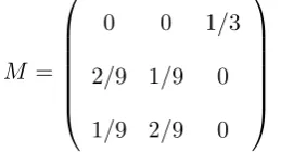
Figure 2.1: The permuton ΦM constructed as an example at the end of
Sec-tion 2.2. The gray area in the picture is the support of the measure and different shades correspond to the density of the measure.
tozi in thei-th row and in the i-th column, we can define a permuton ΦM as
ΦM = k X
i,j=1
MijΥAij ,
whereAij = [si−1, si]×[sj−1, sj],i, j∈[k] and si=z1+· · ·+zi (in particular,
s0 = 0 and sk = 1). For instance, ifz1 =z2 =z3 = 1/3 and
M =
0 0 1/3
2/9 1/9 0
1/9 2/9 0
,
we get the permuton depicted in Figure 2.1.
2.3
Permutons with infinite structure
In this section, we prove Theorem 3 which asserts that permutons with infinite structure Ω→α and Υ→α are finitely forcible for everyα∈(0,1). We start with
proving finite forcibility of Ω→α. We prove finite forcibility of Υ→α later in this
section as Theorem 16.
Theorem 13. For every α∈(0,1), the permuton Ω→α is finitely forcible.
Proof. We claim that any permuton Φ satisfying
t(231,Φ) +t(312,Φ) = 0 , (2.8)
t(21,Φ) = (1−α)2 P∞
i=0
α2i , and (2.9)
R
[0,1]2
1−x−y+FΦ(x, y)−1−αα(x+y−2FΦ(x, y))
2
dΦ = 0 (2.10)
is equal to Ω→α. This would prove the finite forcibility of Ω→αby Theorem 10.
Assume that a permuton Φ satisfies (2.8), (2.9), and (2.10). LetX be the support of Φ and consider the binary relationR defined on the support of Φ such that (x, y)R(x0, y0) if
• x=x0 andy =y0, or
• x < x0 andy > y0, or
• x > x0 andy < y0.
The relation R is an equivalence relation. Indeed, the reflexivity and sym-metry is clear. To prove transitivity, consider three points (x, y), (x0, y0) and (x00, y00) such that (x, y)R(x0, y0) and (x0, y0)R(x00, y00) but it does not hold that
(x, y)R(x00, y00). By the definition ofR, eitherx < x0 andx00< x0, orx > x0 and x00> x0. Ifx < x0 andx00< x0, then we obtain thatt(231,Φ)>0 unlessx=x00
(recall thatR is defined on the support of Φ). We can now assume thatx=x00
andy < y00. Since Φ has uniform marginals, the support of Φ intersects at least one of the open rectangles (0, x)×(y, y00), (x, x0)×(y, y00) and (x0,1)×(y, y00).
However, this yields thatt(231,Φ)>0 in the first two cases andt(312,Φ)>0 in the last case. The casex > x0 and x00 > x0 is handled in an analogous way.
Let Rbe the set of equivalence classes of R. If A∈ R, let Ax and Ay
be the projections of A on the x and y axes. It is not hard to show that Ax
is a closed interval for each A ∈ R and these intervals are internally disjoint for different choices of A ∈ R. The same holds for the projections on the y axis. Since Φ has uniform marginals, the intervals Ax and Ay must have the
same length for everyA∈ R. Moreover, the definition ofR implies that if Ax
precedes A0
x, then Ay also precedes A0y for any A, A0 ∈ R. We conclude that
there exists a setI of internally disjoint closed intervals such that
[
[z,z0]∈I
z, z0= [0,1] and
the support of Φ is equal to (because the density of subpermutations 231 and 312 is zero and the measure Φ has uniform marginals)
[
[z,z0]∈I
(x, z0−x+z), x∈z, z0 .
Note that some intervals contained in I may be formed by single points. Let
I0 be the subset ofI containing the intervals of positive length. Let [z, z0]∈ I
integrated in (2.10) is zero for every (x, y)∈I. Substitutingx+y=z+z0 and
FΦ(x, y) =z into this function implies
z0=z+ (1−α)(1−z) . (2.11)
LetZ be the set formed by the left end points of intervals inI0. Define z1 to be the minimum element of Z, and in general zi to be the minimum
element ofZ\ S
j<i{
zj}. The existence of these elements follows from (2.11) and
the fact that the intervals in I0 are internally disjoint. If Z is finite, we set zk= 1 for k >|Z|. We derive from the definition ofZ and from (2.11) that
I0 =
[zi, zi+ (1−α)(1−zi)], i∈N+ \ {[1,1]} .
Consequently, we obtain
t(21,Φ) =
∞
X
i=1
(1−α)2(1−zi)2= (1−α)2
∞
X
i=1
(1−zi)2 . (2.12)
Forj∈N, we define βj ∈[0,1] as follows:
βj =
1−z1 forj= 1,
1−zj
α(1−zj−1) ifzj 6= 1 and j >1, and 0 otherwise.
The equation (2.12) can now be rewritten as
t(21,Φ) = (1−α)2
∞
X
i=1
α2(i−1)
i Y
j=1
βj2 . (2.13)
Hence, the equality (2.9) can hold only ifβj = 1 for everyj which implies that
zi = 1−αi−1. Consequently, the permutons Φ and Ω→α are identical.
We remark that any permuton Φ obeying the constraints (2.8) and (2.10) must also be equal to Ω→α. However, we decided to include the additional
constraint (2.9) to make the presented arguments more straightforward. Next, we show finite forcibility of the permuton Υ→αfor everyα∈(0,1).
Its structure is similar to that of Ω→α. The proof proceeds along similar lines
as the proof of Theorem 13 but we have to overcome several new technical difficulties.
Lemma 14. There exist a finite set S of permutations and reals γσ, σ ∈ S,
such that the following is equivalent for every permuton Φ:
• P σ∈S
γσt(σ,Φ) = 0,
• Φrestricted to[x1, x2]×[y2, y1]is a (possibly zero) multiple ofΥ[x1,x2]×[y2,y1] for any two points (x1, y1) and (x2, y2) of the support of Φ with x1 < x2
andy1 > y2.
Proof. The proof technique is similar to that used in [61]. For intervalsI, J ⊆ [0,1] and A = I ×J, let υA(X) = υ(X∩A) for every Borel set X ⊆ [0,1]2.
Equivalently,υA(X) =υ(A)·ΥA(X). Let (x1, y1) and (x2, y2) be two points of the support of Φ withx1 < x2 and y1> y2. By Cauchy-Schwarz inequality, the measure Φ restricted [x1, x2]×[y2, y1] is a multiple ofυ[x1,x2]×[y2,y1]if and only if it holds that
Z
(x,y)
Φ([x1, x]×[y2, y])2dυ[x1,x2]×[y2,y1] ×
Z
(x,y)
(x−x1)2(y−y2)2 dυ[x1,x2]×[y2,y1] −
Z
(x,y)
(x−x1)(y−y2)Φ([x1, x]×[y2, y]) dυ[x1,x2]×[y2,y1]
2
= 0 (2.14)
Since the left hand side of (2.14) cannot be negative, we obtain that the second statement in the lemma is equivalent to
Z
(x1,y1) Z
(x2,y2) Z
(x,y)
Z
(x0,y0)
(x0−x1)2(y0−y2)2·Φ ([x1, x]×[y2, y])2−
(x−x1)(y−y2)·Φ ([x1, x]×[y2, y])·(x0−x1)(y0−y2)·Φ([x1, y2]×[x0, y0])
dυ[x1,x2]×[y2,y1]dυ[x1,x2]×[y2,y1]dΦ dΦ = 0 (2.15)
In the rest of the proof, we show that the left hand side of (2.15) can be expressed as a linear combination of finitely many subpermutation densities. Since this argument follows the lines of the proofs of Theorems 9–11, we only briefly explain the main steps.
x1 ≥ x2, y1 ≥ y2, x 6∈ [x1, x2], x0 6∈ [x1, x2], y 6∈ [y1, y2], or y0 6∈ [y1, y2]. Such points (x1, y1), (x2, y2), (x, y), and (x0, y0) can be obtained by sampling six random points from [0,1]2 based on Φ since Φ has uniform marginals (see the proof of Theorem 9 for more details). When the four points (x1, y1), (x2, y2), (x, y), and (x0, y0) are sampled, any of the quantitiesx1,y2,x,y,x0,y0, Φ ([x1, y2]×[x, y]), and Φ([x1, y2]×[x0, y0]) appearing in the product is equal to the probability that a point randomly chosen in [0,1]2 based on Φ has a certain property in a permutation determined by the sampled points. Since we need to sample six additional points to be able to determine each of the products appearing in (2.15),the left hand side of (2.15) is equal to a linear combina-tion of densities of 12-element permutacombina-tions with appropriate coefficients. We conclude that the lemma holds withS =S12.
Analogously, one can prove the following lemma. Since the proof follows the lines of the proof of Lemma 14, we omit further details.
Lemma 15. There exist a finite set S of permutations and reals γσ, σ ∈ S
such that the following is equivalent for every permuton Φ:
• Pσ∈Sγσt(σ,Φ) = 0,
• if (x1, y1), (x2, y2), and (x3, y3) are three points of the support of Φ with x1 < x2 < x3 and y2< y3< y1, then Φrestricted to [x2, x3]×[y2, y3]is a
(possibly zero) multiple ofΥ[x2,x3]×[y2,y3].
We are now ready to show that each permuton Υ→α,α∈(0,1), is finitely
forcible.
Theorem 16. For every α∈(0,1), the permuton Υ→α is finitely forcible.
Proof. LetS be the union of the two sets of permutations from Lemma 14 and Lemma 15. Next, consider the following eight functions:
FΦ-(x, y) = F21
Φ (x, y) , f
-Φ (x, y) = FΦ231(x, y) +FΦ321(x, y) ,
FΦ%(x, y) = F12
Φ (x, y) , f
%
Φ (x, y) = F 231 Φ (x, y) ,
FΦ.(x, y) = F12
Φ (x, y) , f
.
Φ (x, y) = F 312 Φ (x, y) ,
FΦ&(x, y) = F21
Φ (x, y) , f
&
Φ (x, y) = F 312
Φ (x, y) +FΦ321(x, y) .
We claim that any permuton satisfying the following three conditions is equal to Υ→α:
t(σ,Φ) =t(σ,Υ→α) for everyσ ∈S, (2.16)
Z
[0,1]2
(1−α)FΦ%fΦ&−FΦ&fΦ%fΦ
-−α FΦ-fΦ-fΦ&+FΦ&fΦ-fΦ&+FΦ-fΦ.fΦ&+FΦ&fΦ-fΦ%2 dΦ = 0, (2.17)
and
t(21,Φ) = (1−α) 2
2
∞
X
i=0
α2i . (2.18)
This would prove the finite forcibility of Υ→α by Theorem 11.
Suppose that a permuton Φ satisfies (2.16), (2.17), and (2.18). Let X be the support of Φ and consider the binary relationR defined on the support of Φ such that (x, y)R(x0, y0) if
• x=x0 andy =y0,
• x < x0 andy > y0, or
• x > x0 andy < y0.
Unlike in the proof of Theorem 13, the relation R need not be an equivalence relation. Instead, we consider the transitive closureR0 of R and let R be the set of the equivalence classes ofR0.
We defineρ((x, y),(x0, y0)), where (x, y) and (x0, y0) are two points of the support of Φ such that (x, y)R(x0, y0), as follows
ρ (x, y),(x0, y0)=
Φ([x,x0]×[y0,y])
(x0−x)(y−y0) ifx < x0 andy > y0,
Φ([x0,x]×[y,y0])
(x−x0)(y0−y) ifx > x0 andy < y0, and 0 otherwise.
Since Φ satisfies (2.16), Lemma 14 implies that any three points (x, y), (x0, y0) and (x00, y00) of the support of Φ such that (x, y)R(x0, y0) and (x0, y0)R(x00, y00) satisfyρ((x, y),(x0, y0)) =ρ((x0, y0),(x00, y00)). In particular,ρ((x, y),(x0, y0)) has
As in the proof of Theorem 13, we defineAxandAyto be the projections
of an equivalence classA∈ R on thex and y axes. The definition of R yields that Ax and Ay are closed intervals for all A ∈ R and these intervals are
internally disjoint for different choices ofA∈ R. Since Φ has uniform marginals, the intervalsAx and Ay must have the same length for every A∈ R. As in the
proof of Theorem 13, we conclude that there exists a setI of internally disjoint closed intervals such that
[
[z,z0]∈I
[z, z0] = [0,1] ,
the support of Φ is a subset of
[
[z,z0]∈I
[z, z0]×[z, z0] ,
and the interior of each of these squares intersects at most one class A ∈ R. Since some intervals contained inI may be formed by single points, we define
I0 to be the subset ofI containing the intervals of positive length. Let [z, z0]∈ I
0 and letAbe the closure of the corresponding equivalence class fromR. Let f(x),x∈[z, z0], be the minimum y such that (x, y) belongs toA; similarly,g(x) denotes the maximum such y.
Assume first that ρ(A) > 0. Since Φ has uniform marginals, it holds that g(x)−f(x) = ρ(A)−1 for every x ∈ (z, z0). From (2.16) and Lemma 14
we see that the functionsf and gare non-decreasing, and similarly (2.16) and Lemma 15 imply that f and g are non-increasing. We conclude that A = ([z, z0]×[z, z0]) andρ(A) = (z0−z)−1.
Assume now thatρ(A) = 0. Lemma 15 and (2.16) imply that if (x, y)∈
(z, z0)×(z, z0) belongs to the support of Φ, then Φ([x, z0]×[z, y]) = 0 (otherwise,
ρ(A) >0). But then (x, y) cannot be in relation R with another point of the support of Φ. So, we conclude that the caseρ(A) = 0 cannot appear.
The just presented arguments show the support of the measure Φ is equal to
[
[z,z0]∈I
[z, z0]×[z, z0]
and the measure is uniformly distributed inside each square [z, z0]×[z, z0], [z, z0]∈ I
0.
Let [z, z0] be one of the intervals from I0. Recall that we have argued that
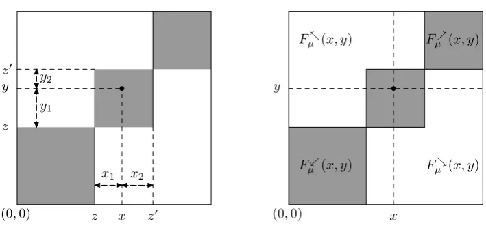
(0,0) z x z0 z
y z0
x1 x2
y1
y2
(0,0) x
y
Fµ-(x, y)
F. µ (x, y)
Fµ%(x, y)
[image:37.595.115.470.64.231.2]F& µ (x, y)
Figure 2.2: Notation used in equalities (2.20) and (2.21). Areas that can contain the support of Φ are drawn in grey.
and the measure Φ is uniform inside the square [z, z0]×[z, z0] (see Figure 2.2).
By (2.17), the following holds for almost every point of the support of Φ:
(1−α)FΦ%fΦ&−FΦ&fΦ%fΦ-=α FΦ-fΦ-fΦ&+FΦ&fΦ-fΦ&+
FΦ-fΦ.fΦ&+FΦ&fΦ-fΦ%. (2.19)
In particular, this holds for all points in [z, z0]×[z, z0] since the functions ap-pearing in (2.19) are continuous.
Let (x, y) be a point from (z, z0)×(z, z0). Let x
1 =x−z,x2 =z0−x, y1=y−z, and y2 =z0−y (see Figure 2.2). Since all the quantities appearing in (2.19) are positive, we may rewrite (2.19) as
(1−α) FΦ%−FΦ&f
%
Φ fΦ&
!
=α FΦ-+FΦ&+FΦ-f
.
Φ fΦ- +F
&
Φ fΦ% fΦ&
!
. (2.20)
Observe thatFΦ%(x, y) = Φ([x,1]×[y,1]),FΦ-(x, y) = Φ([z, x]×[y, z0]) = x1y2 z0−z, andFΦ&(x, y) = Φ([x, z0]×[z, y]) = x2y1
z0−z. Further observe that
fΦ%(x, y) fΦ&(x, y) =
2x2 2y1y2
2(z0−z)2 x2
2y12
(z0−z)2 = y2
y1
and f
.
Φ (x, y) fΦ-(x, y) =
2x2 1y1y2
2(z0−z)2 x2
1y22
(z0−z)2 = y1
y2 .
Plugging these observations in (2.20), we obtain that
(1−α)
Φ([x,1]×[y,1])− x2y2 z0−z
=αx1y2+x2y1+x1y1+x2y2
Sincex1+x2 =y1+y2 =z0−z and zx02−y2z = Φ([x, z0]×[y, z0]), we obtain from (2.21) that
(1−α)Φ([z0,1]×[z0,1]) =α(z
0 −z)2 z0−z =α(z
0
−z) . (2.22)
Finally, we substitute 1−z0 for Φ([z0,1]×[z0,1]) in (2.22) and get the following:
z0=z+ (1−α)(1−z) . (2.23)
So, we conclude that the right end point of every interval in I0 is uniquely determined by its left end point.
Let Z be the set formed by the left end points of intervals in I0. As in the proof of Theorem 13, for a positive integeri, let zi be the i-th smallest
element of Z. Notice that the existence of minimum elements follows from (2.23). IfZ is finite, we set zk = 1 for k >|Z|.
We derive from the definition ofZ and from (2.23) that
I0 =
[zi, zi+ (1−α)(1−zi)], i∈N+ \ {[1,1]} .
Consequently, we obtain
t(21,Φ) =
∞
X
i=1
(1−α)2(1−z
i)2
2 =
(1−α)2 2
∞
X
i=1
(1−zi)2 . (2.24)
Analogously to the proof of Theorem 13, for j ∈ N, we define βj ∈ [0,1] as
follows:
βj =
1−z1 forj= 1,
1−zj
α(1−zj−1) ifzj 6= 1 and j >1, and 0 otherwise.
The equation (2.24) can be rewritten as
t(21,Φ) = (1−α) 2
2
∞
X
i=1
α2(i−1)
i Y
j=1
βj2. (2.25)
Hence, the equality (2.18) can hold only ifβj = 1 for everyj, i.e.,zi = 1−αi−1.
2.4
Graphons with infinite structure
In this section, we show that graphons associated with the finitely forcible permutons from Section 2.3 are not finitely forcible. We start with graphons WΩ→α associated with permutons Ω→α,α∈(0,1).
2.4.1 Union of complete graphs
We now focus on graphons with t(P3, W) = 0 where P3 is the path on three vertices. We start with the following lemma, which seems to be of independent interest. Informally, the lemma asserts that any finitely forcible graphon with zero density ofP3 can be forced by finitely many densities of complete graphs.
Lemma 17. If W0 is a finitely forcible graphon and t(P3, W0) = 0, then there
exists an integer`0 such that any graphonW witht(P3, W) = 0andt(K`, W) =
t(K`, W0) for `≤`0 is weakly isomorphic to W0.
Proof. To prove the statement of the lemma, it is enough to show the following claim: the density of anyn-vertex graphGin a graphon W witht(P3, W) = 0 can be expressed as a combination of densities ofK1, . . .,KninW. We proceed
by induction onn+kwherenandkare the numbers of vertices and components ofG respectively. Ifn=k= 1, there exists only a single one-vertex graphK1 and the claim holds.
Assume now that n+k > 2. If G is not a union of complete graphs, then t(G, W) = 0 since t(P3, W) = 0. So, we assume that G is a union of k complete graphs G1, . . . , Gk, i.e., G = G1 ∪ · · · ∪Gk. If k = 1, then G = Kn
and the claim clearly holds. So, we assumek >1. For 2≤i≤k, we denote
Hi = (G1+Gi)∪ [
j∈[k]\{1,i}
Gj .
Observe that the following holds:
t(G1, W)·t(G2∪ · · · ∪Gk, W) =
p1 · t(G, W) +
k X
i=2
pi · t(Hi, W) (2.26)
where p1 is the probability that a set V of randomly chosen |G1| vertices of the graph G induces a complete graph and the graph G\V is isomorphic to G2∪ · · · ∪Gk, and pi,i >1, is the probability that a set V of randomly chosen |G1|vertices ofHiinduces a complete graph and the graphHi\V is isomorphic