Valuation risk revalued

Valuation Risk Revalued

Valuation Risk Revalued

∗

Oliver de Groot

Alexander W. Richter

Nathaniel A. Throckmorton

October 1, 2018

A

This paper shows the recent success of valuation risk (time-preference shocks in

Epstein-Zin utility) in resolving asset pricing puzzles rests sensitively on an undesirable asymptote that

occurs because the preference specification fails to satisfy a key restriction on the weights in

the Epstein-Zin time-aggregator. In a Bansal-Yaron long-run risk model, our revised valuation

risk specification that satisfies the restriction provides a superior empirical fit. The results also

show that valuation risk no longer has a major role in matching the mean equity premium and

risk-free rate but is crucial for matching the volatility and autocorrelation of the risk-free rate.

Keywords: Epstein-Zin Utility; Valuation Risk; Equity Premium Puzzle; Risk-Free Rate Puzzle

JEL Classifications: D81; G12

∗_{de Groot, School of Economics and Finance, University of St Andrews, St Andrews, Scotland and Monetary}

DE GROOT, RICHTER & THROCKMORTON: VALUATION RISKREVALUED

1 I

In standard asset pricing models, uncertainty enters through the supply side of the economy, either

through endowment shocks in a Lucas (1978) tree model or productivity shocks in a production economy model. Recently, several papers introduced demand side uncertainty or “valuation risk”

as a potential explanation of key asset pricing puzzles (Albuquerque et al. (2016, 2015); Creal and

Wu (2017); Maurer (2012); Nakata and Tanaka (2016); Schorfheide et al. (2018)). In

macroeco-nomic parlance, valuation risk is usually referred to as a discount factor or time preference shock.1 The literature contends valuation risk is an important determinant of key asset pricing moments

when it is embedded in Epstein and Zin (1991) recursive preferences. We show the success of

val-uation risk rests on an undesirable asymptote that permeates the determination of asset prices. The

influence of the asymptote is easily identified in a stylized model. In that model, an intertemporal elasticity of substitution (IES) marginally above one predicts an arbitrarily large equity premium

and an arbitrarily low risk-free rate, while an IES slightly below one predicts the opposite results.

Moreover, the asymptote significantly affects equilibrium outcomes even when the IES is well

above unity by qualitatively changing the relationship between the IES and the equity premium.

de Groot et al. (2018) show that with Epstein-Zin preferences, time-varying weights in a CES

time-aggregator must sum to1to prevent an undesirable asymptote from determining equilibrium

outcomes. The current specification used in the literature fails to impose this important restriction.

de Groot et al. (2018) propose an alternative specification (henceforth, the “revised specification”)

that eliminates the asymptote and ensures that preferences are well-defined when the IES is one.2 This paper uses the revised specification to re-evaluate the role of valuation risk in explaining key asset pricing moments. While the change to the model will appear minor, it profoundly alters

the equilibrium predictions of the model. Key comparative statics, such as the response of the

equity premium and the risk-free rate to a rise in the IES, switch sign. This means that once we

re-estimate the model, the parameters that best fit the data as well as the relative contribution of

valuation risk change dramatically. For example, our baseline model with the revised specification

requires a coefficient of relative risk aversion (RA) well above the accepted range in the literature.

For intuition, consider the log-stochastic discount factor (SDF) under Epstein-Zin preferences

ˆ

mt+1 =θlogβ+θ(ˆat−ωˆat+1)−(θ/ψ)∆ˆct+1+ (θ−1)ˆry,t+1, (1)

where the first, third, and fourth terms—the subjective discount factor (β), log-consumption growth

(∆ˆct+1), and the log-return on the endowment (rˆy,t+1)—are all standard in this class of asset pricing

models. The second term captures valuation risk, where ˆat is a time preference shock. In the

1_{Time preference shocks have been widely used in the macro literature (e.g., Christiano et al. (2011); Eggertsson}

DE GROOT, RICHTER & THROCKMORTON: VALUATION RISKREVALUED

current literature,ω = 0. Once we revise the preferences and re-derive the log-SDF, we findω =β.

When we apply this single alteration to the model, the asset pricing predictions are starkly different.

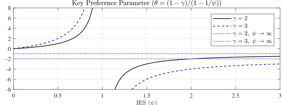
The asymptote in the current valuation risk specification is related to the preference parameter θ ≡(1−γ)/(1−1/ψ)that enters the log-SDF, whereγ is RA andψ is the IES. Under constant relative risk aversion (CRRA) preferences,γ = 1/ψ. In this case,θ= 1and the log-SDF becomes

ˆ

mt+1 = logβ+ (ˆat−ωˆat+1)−∆ˆct+1/ψ. (2)

The return on the endowment drops out of (1), so the log-SDF is simply composed of the subjective

discount factor and consumption growth terms. The advantage of Epstein-Zin preferences is that

they decoupleγ andψ, so it is possible to simultaneously have high RA and a high IES. However,

there is a nonlinear relationship between θ and ψ, as shown in figure 1. A vertical asymptote

occurs at ψ = 1: θ tends to infinity as ψ approaches 1from below while the opposite occurs as ψ approaches 1from above. When the IES equals 1, θ is undefined. In addition to the vertical asymptote inθ, there is also a horizontal asymptote at1−γ as the IES becomes perfectly elastic.

0 0.5 1 1.5 2 2.5 3

-8 -6 -4 -2 0 2 4 6 8

Figure 1: Preference parameterθin the stochastic discount factor from a model with Epstein-Zin preferences.

Under Epstein and Zin (1989) preferences and the generalization in de Groot et al. (2018) to

include valuation risk, the asymptote infigure 1does not affect asset prices. There is a well-defined

equilibrium when the IES equals1and asset pricing predictions are robust to small variations in

the IES around1. Continuity is preserved because the weights in the time-aggregator always sum

to unity. An alternative interpretation is that the time-aggregator maintains the well-known

prop-erty that a CES aggregator tends to a Cobb-Douglas aggregator as the elasticity approaches1. The

current specification violates the restriction on the weights so the limiting properties of the CES aggregator break down. As a result, the asymptote infigure 1permeates key asset pricing moments.

Taken at face value, the asymptote that occurs with the current specification resolves the equity

(Camp-DE GROOT, RICHTER & THROCKMORTON: VALUATION RISKREVALUED

bell and Cochrane (1999)). Furthermore, when we estimate a model that includes valuation risk and

a small long-run predictable component in consumption and dividend growth (henceforth,

“long-run risk) following Bansal and Yaron (2004), counterfactual exercises demonstrate that asset prices

are almost completely explained by valuation risk, rather than long-run risk. The reason is that

val-uation risk is able to match the mean equity premium and risk-free rate while maintaining a low

cor-relation between the equity return and consumption and dividend (henceforth, cash flow) growth.

We summarize our main results as follows: (1) The current valuation risk specification fits the data well due to an undesirable asymptote; (2) In our baseline model, the revised specification does

not perform as well; (3) When we add Bansal-Yaron long-run risk, revised valuation risk is

impor-tant for matching the volatility and autocorrelation of the risk-free rate but plays only a minor role

in determining most asset pricing moments. Nevertheless, the revised specification fits the data

bet-ter than the current specification in this model. This is because revised valuation risk has a distinct

role, matching the dynamics of the risk-free rate while long-run risk captures the other moments;

(4) Extending the model so valuation risk shocks directly affect cash flow growth further improves

the empirical fit and helps resolve the correlation puzzle. Conditional on the set of data moments we match, we show this extension is statistically preferred to the addition of stochastic volatility.

The paper proceeds as follows. Section 2 describes the baseline model and the current and

revised preference specifications. Section 3 analytically shows why asset prices depend so

dra-matically on the way valuation risk enters the Epstein-Zin utility function. Section 4quantifies the

effects of the valuation risk specification in our baseline model. Section 5estimates the relative

im-portance of valuation and long-run risk.Section 6extends our long-run risk model to include

valua-tion risk shocks to cash flow growth and stochastic volatility on cash flow risk.Section 7concludes.

2 B

A

-P

M

We begin by describing our baseline model. Each periodtdenotes1month. There are two assets: an endowment share,s1,t, that pays income,yt, and is in fixed unit supply, and an equity share,s2,t,

that pays dividends,dt, and is in zero net supply. The agent chooses{ct, s1,t, s2,t}∞t=0 to maximize

U_tC = [(1−β)c(1t −γ)/θ+aCt β(Et[(UtC+1)1

−_γ

])1/θ]θ/(1−_γ)

, 16=ψ >0, (3)

as used in the current (C) asset pricing literature, or

U_tR=

  

[(1−aR t β)c

(1−_γ)/θ

t +aRt β(Et[(UtR+1)1

−_γ

])1/θ_]θ/(1−_γ)

, for16=ψ >0,

c1−aRtβ

t (Et[(UtR+1)1

−_γ ])aR

tβ/(1−γ), forψ = 1,

(4)

DE GROOT, RICHTER & THROCKMORTON: VALUATION RISKREVALUED

denotedaC

t >0and0< aRt <1/β.3,4 The key difference between the preferences is as follows:

The time-varying weights of the time-aggregator in (3),(1−β)andaC t β, do

not sum to1, whereas the weights in (4),(1−aR

t β)andaRt β, do sum to1.

The representative agent’s choices are constrained by the flow budget constraint given by

ct+py,ts1,t+pd,ts2,t = (py,t+yt)s1,t−₁+ (p_d,t+d_t)s_2,t−₁, (5)

wherepy,tandpd,tare the endowment and dividend claim prices. The optimality conditions imply

Et[mjt+1ry,t+1] = 1, ry,t+1 ≡(py,t+1+yt+1)/py,t, (6)

Et[mjt+1rd,t+1] = 1, rd,t+1 ≡(pd,t+1+dt+1)/pd,t, (7)

wherej ∈ {C, R},ry,t+1 andrd,t+1are the gross returns on the endowment and dividend claims,

mC_t+1 ≡aC_t β

ct+1 ct

−1/ψ (VC

t+1)1

−γ

Et[(VtC+1)1−γ]

1−1 θ

, (8)

mR

t+1 ≡aRt β

1−aR t+1β 1−aR

tβ

ct+1 ct

−_1/ψ (VR

t+1)1

−_γ

Et[(VtR+1)1

−_γ ]

1−1 θ

, (9)

andV_tj is the value function that solves the agent’s constrained optimization problem.

To permit an approximate analytical solution, we rewrite (6) and (7) as follows

Et[exp( ˆmjt+1+ ˆry,t+1)] = 1, (10)

Et[exp( ˆmjt+1+ ˆrd,t+1)] = 1, (11)

wheremˆj_t+1 is defined in (1) andˆat ≡ ˆaCt ≈ ˆaRt /(1−β)so the shocks in the current and revised

models are directly comparable. The common time preference shock,ˆat+1, evolves according to

ˆ

at+1 =ρaˆat+σaεa,t+1, εa,t+1 ∼N(0,1), (12)

where0≤ ρa <1is the persistence of the process,σa ≥0is the shock standard deviation, and a

hat denotes a log variable. We then apply a Campbell and Shiller (1988) approximation to obtain

ˆ

ry,t+1 =κy0+κy1zˆy,t+1−zˆy,t+ ∆ˆyt+1, (13)

ˆ

rd,t+1 =κd0+κd1zˆd,t+1−zˆd,t+ ∆ ˆdt+1, (14)

3_{Kollmann (2016) introduces a time-varying discount factor in an Epstein-Zin setting similar to our formulation. In}

that setup, the discount factor is a function of endogenously determined consumption rather than a stochastic process. 4_{In the literature,a}C

t typically hits current utility, rather than the risk aggregator. However, with a small change in

DE GROOT, RICHTER & THROCKMORTON: VALUATION RISKREVALUED

wherezˆy,t+1 is the price-endowment ratio,zˆd,t+1is the price-dividend ratio, and

κy0 ≡log(1 + exp(ˆzy))−κy1zˆy, κy1 ≡exp(ˆzy)/(1 + exp(ˆzy)), (15)

κd0 ≡log(1 + exp(ˆzd))−κd1zˆd, κd1 ≡exp(ˆzd)/(1 + exp(ˆzd)), (16)

are constants that are functions of the steady-state price-endowment and price-dividend ratios.

To close the model, the processes for log-endowment and log-dividend growth are given by

∆ˆyt+1 =µy+σyεy,t+1, εy,t+1 ∼N(0,1), (17)

∆ ˆdt+1 =µd+πdyσyεy,t+1+ψdσyεd,t+1, εd,t+1∼N(0,1), (18)

whereµy andµd are the steady-state growth rates, σy ≥ 0 andψdσy ≥ 0are the shock standard

deviations, and πdy captures the covariance between consumption and dividend growth. Asset

market clearing impliess1,t = 1ands2,t = 0, so the resource constraint is given byˆct= ˆyt.

Equilibrium includes sequences of quantities{ˆct}∞t=0, prices {mˆt+1,zˆy,t,zˆd,t,rˆy,t+1,rˆd,t+1}∞t=0

and exogenous variables{∆ˆyt+1,∆ ˆdt+1,ˆat+1}∞t=0 that satisfy (1), (10)-(14), (17), (18), and the

re-source constraint, given the state of the economy,{ˆat}, and sequences of shocks,{εy,t, εd,t, εa,t}∞t=1. We posit the following solutions for the price-endowment and price-dividend ratios:

ˆ

zy,t=ηy0+ηy1aˆt, zˆd,t=ηd0+ηd1ˆat, (19)

wherezˆy = ηy0 andzˆd =ηd0. We solve the model with the method of undetermined coefficients.

Appendix Bderives the SDF, a Campbell-Shiller approximation, the solution, and key asset prices.

3 I

This section develops intuition for why the valuation risk specification has such large effects on

the model predictions. To simplify the exposition, we consider different stylized shock processes.

3.1 CONVENTIONAL MODEL First, it is useful to review the role of Epstein-Zin preferences and

the separation of the RA and IES parameters in matching the risk-free rate and equity premium. For

simplicity, we remove valuation risk (σa = 0) and assume endowment/dividend risk is perfectly

correlated (ψd = 0;πdy = 1). The average risk-free rate and average equity premium are given by

E[ˆrf] =−logβ+µy/ψ+ ((1/ψ−γ)(1−γ)−γ2)σy2/2, (20)

E[ep] =γσ_y2, (21)

where the first term in (20) is the subjective discount factor, the second term accounts for

DE GROOT, RICHTER & THROCKMORTON: VALUATION RISKREVALUED

an incentive for agents to borrow in order to smooth consumption. Since both assets are in fixed

supply, the risk-free rate must be elevated to deter borrowing. When the IES,ψ, is high, agents are

willing to accept higher consumption growth so the interest rate required to dissuade borrowing is

lower. Therefore, the model requires a fairly high IES to match the low risk-free rate in the data.

With CRRA preferences, higher RA lowers the IES and pushes up the risk-free rate. With

Epstein-Zin preferences, these parameters are independent, so a high IES can lower the risk-free

rate without lowering RA. Notice the equity premium only depends on RA. Therefore, the model generates a low risk-free rate and modest equity premium with sufficiently high RA and IES

param-eter values. Of course, there is an upper bound on what constitute reasonable RA and IES values,

which is the source of the risk-free rate and equity premium puzzles. Other prominent features such

as long-run risk and stochastic volatility `a la Bansal and Yaron (2004) help resolve these puzzles.

3.2 VALUATION RISK MODEL Now consider an example where we remove cash flow risk

(σy = 0;µy = µd) and also assume the time preference shocks are i.i.d. (ρa = 0). Under these

assumptions, the assets are identical so(κy0, κy1, ηy0, ηy1) = (κd0, κd1, ηd0, ηd1)≡(κ0, κ1, η0, η1).

Current Specification We first solve the model with the current preferences, so the SDF is given by (1) withω = 0. In this case, the average risk-free rate and average equity premium are given by

E[ˆrf] =−logβ+µy/ψ+ (θ−1)κ21η21σa2/2, (22)

E[ep] = (1−θ)κ2

1η12σa2. (23)

It is also straightforward to show the log-price-dividend ratio is given byzˆt=η0+ ˆat(i.e., the

loading on the preference shock,η1, is1). Therefore, when the agent becomes more patient andaˆt

rises, the price-dividend ratio rises one-for-one on impact and returns to the stationary equilibrium

in the next period. Sinceη1is independent of the IES, there is no endogenous mechanism that

pre-vents the asymptote inθfrom influencing the risk-free rate or equity premium. It is easy to see from

(16) that 0 < κ1 < 1. Therefore, θ dominates the average risk-free rate and average equity

pre-mium when the IES is near1. The following result describes the comparative statics with the IES:

As ψ approaches 1 from above, θ tends to −∞. As a result, the average

risk-free rate tends to−∞while the average equity premium tends to+∞.

This key finding illustrates why valuation risk seems like such an attractive feature for resolving

the risk-free rate and equity premium puzzles. As the IES tends to 1from above, θ becomes

in-creasingly negative, which dominates other determinants of the risk-free rate and equity premium.

In particular, with an IES slightly above1, the asymptote in θcauses the average risk-free rate to

DE GROOT, RICHTER & THROCKMORTON: VALUATION RISKREVALUED

IES marginally below 1 (a popular value in the macro literature), generates the opposite

predic-tions. As the IES approaches infinity,θ−1tends toγ. Therefore, even when the IES is far above 1, the last term in (22) and (23) is scaled byγand can still have a meaningful effect on asset prices. An IES equal to 1 is a key value in the asset pricing literature. For example, it is the basis

of the “risk-sensitive” preferences in Hansen and Sargent (2008, section 14.3). Therefore, it is a

desirable property for small perturbations around an IES of1to not materially alter the predictions

of the model. A well-known example of where this property holds is the standard Epstein-Zin asset pricing model without valuation risk. Even though the log-SDF as written in (2) is undefined when

the IES equals1, both the risk-free rate and the equity premium in (20) and (21) are well-defined.

Revised Specification Next we solve the model with the revised preferences, so the SDF is given

by (1) withω =β. In this case, the average risk-free rate and average equity risk premium become

E[ˆrf] = −logβ+µy/ψ+ ((θ−1)κ21η12−θβ2)σa2/2, (24)

E[ep] = ((1−θ)κ1η1+θβ)κ1η1σ2a. (25)

Relative to the current specification, the preference shock loading,η1, is unchanged. However,

both asset prices include a new term that captures the direct effect of valuation risk on current

util-ity, so a rise inat that makes the agent more patient raises the value of future certainty equivalent

consumption and lowers the value of present consumption. The asymptote occurs with the current

specification because it does not account for the effect of valuation risk on current consumption. With the revised preferences,κ1 =βwhenψ = 1, so the terms involvingθ cancel out and the

asymptote disappears.5 _{The presence of valuation risk lowers the average risk-free rate byβ}2_σ2 a/2 and raises the average equity return by the same amount. Therefore, the average equity premium

equalsβ2_σ2

a, which is invariant to the level of RA. When ψ > 1, κ1 > β, so an increase in RA lowers the risk-free rate and raises the equity return. Asψ → ∞, the ratio of the equity premium

with revised specification relative to the current specification equals 1 +β(1−γ)/(γκ1). This

means the disparity between the predictions of the two models grows as the level of RA increases.

Expected utility With CRRA preferences (γ = 1/ψ), the specifications in (3) and (4) reduce to

U_tC =EtP

∞

j=0(1−β)(

Qj

i=1aCt+i−1)β

j_c1−γ

t+j/(1−γ),

U_tR=EtP

∞

j=0(1−βaRt+j)( Qj

i=1aRt+i−₁)β

j_c1−_γ

t+j/(1−γ).

There is no longer an asymptote with the current preferences becauseθ= 1with CRRA utility. The

current and revised specifications also generate identical impulse responses to a time preference

5_Noticeκ

1is a convolution of the steady-state price-dividend ratio,zd. When the IES is1,zd=β/(1−β), which is

DE GROOT, RICHTER & THROCKMORTON: VALUATION RISKREVALUED

shock sinceη1 = 1. However, the two specifications still have different asset pricing implications.

Under the current specification, valuation risk has no effect on the risk-free rate and there is no

equity premium. With the revised specification, the presence of valuation risk lowers the average

risk-free rate byβ2_σ2

a/2and the average equity premium equalsβ2σa2, just like when the IES equals unity with EpsteZin preferences. Therefore, the two expected utility specifications are not

in-terchangeable, but the quantitative differences are insignificant. We can also conclude that the

asymptote and stark differences in asset prices between the two Epstein-Zin preference specifica-tions come through the continuation value,Vt+1, in the SDF, which drops out with expected utility.

0.5 1 1.5 2 2.5 3 0

2 4 6 8

0.5 1 1.5 2 2.5 3 -1

-0.5 0 0.5 1

0.5 1 1.5 2 2.5 3 0.995

0.996 0.997 0.998 0.999 1

0 0.1 0.2 0.3 0.4 0.5 0.02

0.025 0.03

ψ→ ∞

(Current Preferences)

Figure 2: Equilibrium outcomes in the model without cash flow risk (σy = 0;µy =µd) and i.i.d. preference shocks

(ρa= 0) under the current (C) and revised (R) preference specifications. We setβ = 0.9975,γ= 10, andσa = 0.005.

3.3 ILLUSTRATION Our analytical results show the way a time preference shock enters

Epstein-Zin utility determines whether the asymptote inθshows up in equilibrium outcomes.Figure 2

illus-trates our results by plotting the average risk-free rate, the average equity premium, andκ1(i.e., the marginal response of the price-dividend ratio on the equity return). We focus on the setting in

sec-tion 3.2and plot the results under both preferences with and without endowment/dividend growth.

With the current preferences, the average risk-free rate and average equity premium exhibit a

vertical asymptote when the IES is1, regardless of whetherµy is positive. As a result, the risk-free

rate approaches positive infinity as the IES approaches1from below and negative infinity as the

IES approaches1from above. The equity premium has the same comparative statics with the

oppo-site sign, except there is a horizontal asymptote as the IES approaches infinity. These results occur

because the current specification misses the direct effect of valuation risk on current consumption.6 In contrast, with the revised preferences the average risk-free rate and average equity premium

are continuous in the IES, regardless of the value ofµy. Whenµy = 0, the endowment stream is

6_{Pohl et al. (2018) find the errors from a Campbell-Shiller approximation of the nonlinear model can significantly}

DE GROOT, RICHTER & THROCKMORTON: VALUATION RISKREVALUED

constant. This means the agent is indifferent about the timing of when the preference uncertainty is

resolved, so bothκ1and the average equity premium are independent of the IES. Whenµy >0, the

agent’s incentive to smooth consumption interacts with uncertainty about how (s)he will value the

higher future endowment stream.7 When the IES is large, the agent has a stronger preference for an early resolution of uncertainty, so the equity premium rises as a result of the valuation risk (see

thefigure 2inset). Therefore, the qualitative relationship between the IES and the equity premium

has different signs under the current and revised specifications. However, the increase in the equity premium is quantitatively small and converges to a level significantly below the value with the

current preferences. It is this difference in the sign and magnitude of the relationship between the

IES and the equity premium that will explain many of the empirical results in subsequent sections.

4 E

B

M

This section returns to the baseline model insection 2, which has both valuation and cash flow risk.

We compare the estimates from the model with the current and revised preference specifications.

4.1 DATA ANDESTIMATIONMETHOD We construct our data using the procedure in Bansal and

Yaron (2004), Beeler and Campbell (2012), Bansal et al. (2016), and Schorfheide et al. (2018). The

moments are based on five time series: real per capita consumption expenditures on nondurables

and services, the real equity return, real dividends, the real risk-free rate, and the price-dividend

ra-tio. Nominal equity returns are calculated with the CRSP value-weighted return on stocks. We

ob-tain data with and without dividends to back out a time series for nominal dividends. Both series are

converted to real using the consumer price index (CPI). The nominal risk-free rate is based on the

CRSP yield-to-maturity on90-day Treasury bills. We first convert the nominal series to real using

the CPI. Then we construct an ex-ante real rate by regressing the ex-post real rate on the nominal

rate and inflation over the last year. The consumption data is annual. We convert the monthly asset pricing data to annual series using data from the last month of each year. The model is estimated

using annual data from 1929 to 2017—the longest time span available without combining sources.

We estimate each model in two stages. In the first stage, we use Generalized Method of

Mo-ments (GMM) to obtain point estimates and a variance-covariance matrix of key moMo-ments in the

data. In the second stage, we use Simulated Method of Moments (SMM) to search for the

param-eter vector, θ, that minimizes the squared distance between the GMM point estimates, Ψ˜D, and

median short-sample model moments,Ψ¯M. The weighting matrix,WD, is the inverse diagonal of

the GMM estimate of the variance-covariance matrix,Σ˜D. The objective function,J, is given by

J(θ) = [ ¯ΨM(θ)−Ψ˜D]′WD[ ¯ΨM(θ)−Ψ˜D]/NM,

DE GROOT, RICHTER & THROCKMORTON: VALUATION RISKREVALUED

where we normalize by the number of moments,NM, soJ reflects the average distance from the

moments inΨ˜D. We use simulated annealing and then recursively apply Matlab’sfminsearch

to minimizeJsince gradient-based methods alone did not sufficiently search the parameter space.

Following Albuquerque et al. (2016), our algorithm matches the following 19moments: the

mean and standard deviation of consumption growth, dividend growth, real stock returns, the real

risk-free rate, and the price-dividend ratio, the correlation between dividend growth and

consump-tion growth, the correlaconsump-tion between equity returns and both consumpconsump-tion and dividend growth at a1-,5-, and10-year horizon, and the autocorrelation of the price-dividend ratio and real risk-free

rate. Appendix DandAppendix Eprovide more information about our data and estimation method.

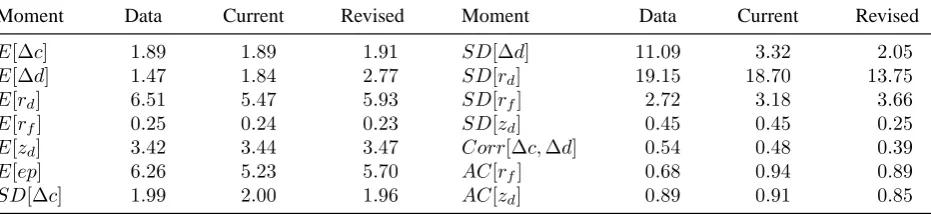
Parameter Current Revised Parameter Current Revised

γ 1.62617 188.36334 µd 0.00190 0.00220 ψ 1.75990 3.53829 ψd 4.25999 4.30687 β 0.99807 0.99364 πdy −0.01606 −0.65893 σy 0.00395 0.00378 σa 0.00028 0.03198 µy 0.00167 0.00171 ρa 0.99701 0.99182

(a) Parameter estimates. Current specification:J= 1.12; Revised specification:J= 1.87.

Moment Data Current Revised Moment Data Current Revised

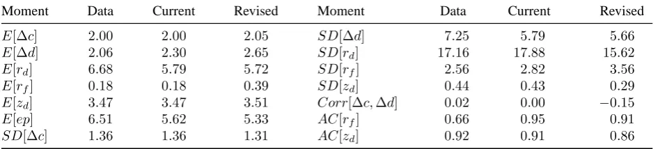
E[∆c] 2.00 2.00 2.05 SD[∆d] 7.25 5.79 5.66

E[∆d] 2.06 2.30 2.65 SD[rd] 17.16 17.88 15.62 E[rd] 6.68 5.79 5.72 SD[rf] 2.56 2.82 3.56 E[rf] 0.18 0.18 0.39 SD[zd] 0.44 0.43 0.29 E[zd] 3.47 3.47 3.51 Corr[∆c,∆d] 0.02 0.00 −0.15 E[ep] 6.51 5.62 5.33 AC[rf] 0.66 0.95 0.91 SD[∆c] 1.36 1.36 1.31 AC[zd] 0.92 0.91 0.86

(b) Unconditional short-sample moments given the parameter estimates for each model.

Table 1: Baseline model estimates and asset pricing moments.

4.2 PARAMETER ESTIMATES AND MOMENTS Table 1shows the estimated parameter values

and selected data and model moments under the current and revised valuation risk specifications.8 The current estimates are very similar to the values reported in Albuquerque et al. (2016), despite

major differences in the data construction. The current model (J = 1.12) fits the data better than

the revised model (J = 1.87). Furthermore, the revised model solved with the current estimates fits the data very poorly (J = 52.61), demonstrating that the two specifications yield sharply different

quantitative predictions. The current model requires a remarkably low RA value (1.6). The low RA

value is due to the asymptote in the current valuation risk specification. An IES close to1raises the

equity premium to an arbitrarily large extent, while IES values further from1cause the equity

pre-8_{Our data sample effectively begins in 1940 because the long-run correlations shorten our sample by10years.}

DE GROOT, RICHTER & THROCKMORTON: VALUATION RISKREVALUED

mium to asymptote at a value much higher than the revised specification generates. Therefore, the

current model is able to maintain a very low RA value while matching key asset pricing moments.

The revised model requires extreme parameter values to match the data, similar to a model

that only includes transitory cash flow risk. For example, the RA estimate (188.4) is an order of

magnitude larger than what is usually accepted in the asset pricing literature.9 Furthermore, the standard deviation of the preference shock is more than two orders of magnitude larger than the

estimate in the current model. Despite these extreme parameter values, the revised model is unable to generate a low enough risk-free rate or a high enough equity premium to match the data. The

elevated parameter values also cause the revised model to underpredict the variance of the equity

return and overpredict the variance of the risk-free rate. The results demonstrate that valuation risk

is not as successful at solving long-standing asset pricing puzzles as the current literature suggests.

5 E

L

-R

R

M

In the baseline model, valuation risk explains most of the key asset pricing moments, even after

cor-recting the preference specification. However, the prominent role of valuation risk is not surprising given that we have abstracted from long-run cash flow risk, which is a well-known potential

resolu-tion of many asset pricing puzzles. Therefore, this secresolu-tion introduces long-run risk to our baseline

model and re-examines the role of valuation risk with both the current and revised preferences.

In order to introduce long-run risk, we modify (17) and (18) as follows:

∆ˆyt+1 =µy + ˆxt+σyεy,t+1, εy,t+1 ∼N(0,1), (26)

∆ ˆdt+1 =µd+φdxˆt+πdyσyεy,t+1+ψdσyεd,t+1, εd,t+1 ∼N(0,1), (27)

ˆ

xt+1 =ρxxˆt+ψxσyεx,t+1, εx,t+1 ∼N(0,1), (28)

where the specification of the persistent component,xˆt, which is common to both the endowment and dividend growth processes, follows Bansal and Yaron (2004). We apply the same estimation

procedure as the baseline model, except we estimate three additional parameters,φd,ρx, andψx.10

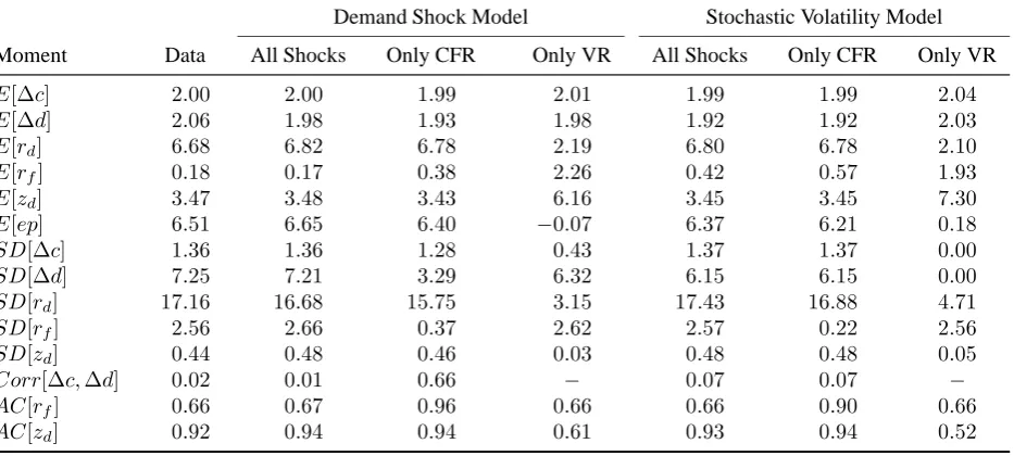
Table 2reproduces the results from the baseline model for the model with long-run risk. With

the current specification, the presence of long-run risk has almost no effect on the ability of the

model to fit the data—theJ value is1.11, compared with1.12in the baseline model (despite three

new parameters). The parameter estimates are also similar to the baseline model and xtdoes not

really provide long run risk to cash flows with an estimated persistence parameter,ρx, of only0.49.

Next, we decompose the role of valuation risk and cash flow risk in explaining the asset pricing

9_{Mehra and Prescott (1985) suggest restricting RA to a maximum of10. The acceptable range for the IES is less} clearly defined in the literature, but values above3are atypical. Both revised estimates are well outside of these ranges.

10_{Long-run risk adds one additional state variable,xˆ}

t. Following the guess and verify procedure applied to the

DE GROOT, RICHTER & THROCKMORTON: VALUATION RISKREVALUED

Parameter Current Revised Parameter Current Revised

γ 1.50849 2.82881 πdy −0.93531 −5.52759 ψ 1.53447 3.95238 σa 0.00027 0.01484 β 0.99822 0.99835 ρa 0.99707 0.95152 σy 0.00382 0.00168 φd 10.82369 1.71444 µy 0.00166 0.00167 ρx 0.49798 0.99932 µd 0.00188 0.00160 ψx 0.15588 0.06208

ψd 2.77760 8.14652 − − −

(a) Parameter estimates. Current specification:J= 1.11; Revised specification:J= 0.36.

Current Specification Revised Specification

Moment Data All Shocks Only CFR Only VR All Shocks Only CFR Only VR

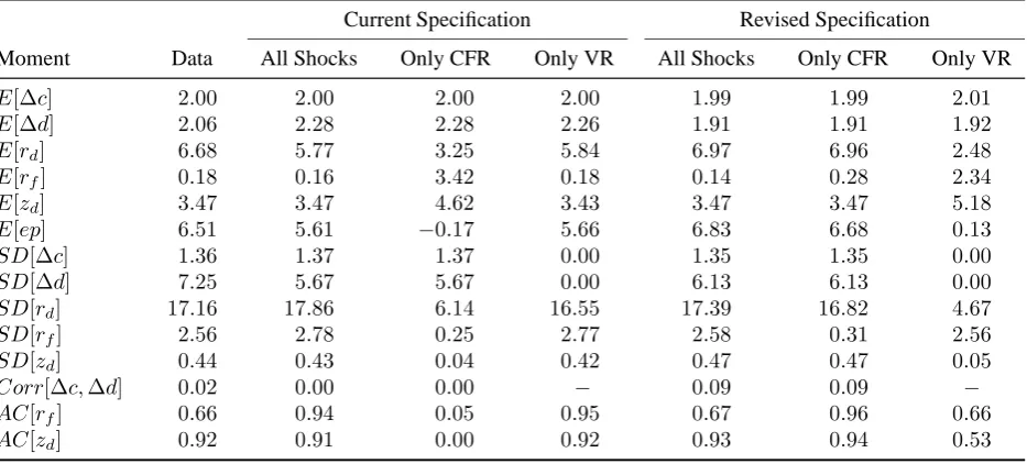
E[∆c] 2.00 2.00 2.00 2.00 1.99 1.99 2.01

E[∆d] 2.06 2.28 2.28 2.26 1.91 1.91 1.92

E[rd] 6.68 5.77 3.25 5.84 6.97 6.96 2.48 E[rf] 0.18 0.16 3.42 0.18 0.14 0.28 2.34 E[zd] 3.47 3.47 4.62 3.43 3.47 3.47 5.18 E[ep] 6.51 5.61 −0.17 5.66 6.83 6.68 0.13

SD[∆c] 1.36 1.37 1.37 0.00 1.35 1.35 0.00

SD[∆d] 7.25 5.67 5.67 0.00 6.13 6.13 0.00

SD[rd] 17.16 17.86 6.14 16.55 17.39 16.82 4.67 SD[rf] 2.56 2.78 0.25 2.77 2.58 0.31 2.56 SD[zd] 0.44 0.43 0.04 0.42 0.47 0.47 0.05 Corr[∆c,∆d] 0.02 0.00 0.00 − 0.09 0.09 −

AC[rf] 0.66 0.94 0.05 0.95 0.67 0.96 0.66 AC[zd] 0.92 0.91 0.00 0.92 0.93 0.94 0.53

(b) Unconditional short-sample moments given the parameter estimates. All Shocks simulates the model with all of the shocks turned on, Only CFR solves and simulates the model with only the cash flow risk shocks, and Only VR solves and simulates the model with only the valuation risk shocks.

Table 2: Long-run risk model estimates and asset pricing moments.

moments. In addition to showing the estimated moments from the entire model (column entitled

All Shocks),table 1breports the moments from two counterfactual simulations that either remove

valuation risk (Only CFR) or cash flow risk (Only VR) from the model. In each case, we re-solve

the models after settingσa = 0for Only CFR andσy = 0for Only VR, so agents make decisions

subject to only one type of risk.11 Since the asymptote resulting from the current valuation risk specification continues to dominate the determination of asset prices, long run risk plays only a

mi-nor role. Valuation risk alone explains almost all of the asset pricing moments, including the near-zero risk free rate and6.5%equity premium. Without valuation risk, the model generates almost

no equity premium, a3.4%risk-free rate, and equity return volatility much lower than in the data.

The results change dramatically with the revised specification in four key ways. One, the model

with long-run risk fits the data much better than the baseline model (theJ value falls from1.87to 0.36) and the parameter estimates are consistent with Bansal and Yaron (2004). Two, with long-run

DE GROOT, RICHTER & THROCKMORTON: VALUATION RISKREVALUED

risk, the revised specification fits the data better than the current specification (with aJ value of 0.36compared to1.11), in contrast with the results from the baseline model. A way to understand this result is to think of the current specification as competing with long-run risk to explain key

asset pricing moments. In contrast, the revised specification complements the original long-run

risk model, in that valuation risk is able to match moments that long-run risk struggles to match.

Three, RA declines from188.4in the baseline model to2.8in the model with long-run risk, well

within the acceptable range in the literature. Four, the decomposition shows that valuation risk no longer explains the vast majority of asset pricing moments. Cash flow risk by itself generates an

equity premium close to the data even though the RA parameter is quite low, whereas valuation risk

alone generates almost no equity premium. Instead, valuation risk plays an important role because

it explains aspects of the risk-free rate. The standard deviation and autocorrelation of the risk-free

rate in the data are2.6%and0.66, whereas long-run risk alone generates values of0.31%and0.96.

We conclude that while valuation risk no longer has the ability to unilaterally resolve long-standing

asset pricing puzzles in its revised form, it remains an important aspect of a long-run risk model.

Current Specification Revised Specification

Moment Data All Shocks Only CFR All Shocks Only CFR

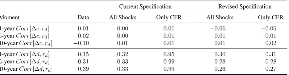
1-yearCorr[∆c, rd] 0.01 0.00 0.01 −0.06 −0.06

5-yearCorr[∆c, rd] −0.02 0.00 0.01 −0.01 −0.01

10-yearCorr[∆c, rd] −0.10 0.01 0.01 0.01 0.02

1-yearCorr[∆d, rd] 0.15 0.32 0.95 0.30 0.31

5-yearCorr[∆d, rd] 0.31 0.33 0.99 0.28 0.28

10-yearCorr[∆d, rd] 0.39 0.33 0.99 0.26 0.27

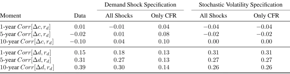
Table 3: Unconditional short-sample moments given the parameter estimates. All Shocks simulates the model with all of the shocks turned on and Only CFR solves and simulates the model with only the cash flow risk shocks.

The Correlation Puzzle Another important asset pricing puzzle pertains to the correlation be-tween equity returns and fundamentals (Cochrane and Hansen (1992)). In the data, the correlation

between equity returns and consumption growth is near zero, regardless of the horizon. The

corre-lation between equity returns and dividend growth is small over short horizons but increases over

longer horizons. The central issue is that many asset-pricing models predict too strong of a

correla-tion between stock returns and fundamentals relative to the data. Clearly, if valuacorrela-tion risk generates

meaningful volatility in asset returns and yet is uncorrelated with consumption and dividend growth

(as in the model insection 2), then valuation risk has the potential to resolve the correlation puzzle.

Table 3 shows the correlations between equity returns and fundamentals over 1-, 5-, and10 -year horizons in the data and the model. We also consider a counterfactual with only cash flow risk

(Only CFR). The correlations with consumption growth are similar across the current and revised

DE GROOT, RICHTER & THROCKMORTON: VALUATION RISKREVALUED

all horizons. With both specifications, cash flow risk is sufficient for the model to match the

data. The correlations with dividend growth are also similar across the two specifications, but their

sources differ. With the current specification, the low correlations are driven by the importance of

valuation risk in the model whereas cash flow risk alone overpredicts the correlation. In contrast,

cash flow risk plays the primary role with the revised specification. The intuition for these results is

straightforward. In a model with long-run risk, most of the volatility in equity returns comes from

changes in consumption and dividend growth, while valuation risk is relegated to a secondary role.

6 E

E

L

-R

R

M

This section further examines the role of valuation risk by extending the model with long-run risk

and the revised valuation risk specification in two independent ways. First, we consider an

exten-sion where valuation risk shocks directly affect consumption and dividend growth, in addition to

their effect on asset prices through the SDF (henceforth, the “Demand” shock model). This feature

is similar to a discount factor shock in a Dynamic Stochastic General Equilibrium (DSGE) model.

For example, in the workhorse New Keynesian model, an increase in the discount factor looks like a typical negative demand shock that lowers interest rates, inflation, and consumption.

There-fore, it provides another potential mechanism for valuation risk to help fit the data, especially the

correlation moments. Following Albuquerque et al. (2016), we augment (26) and (27) as follows:

∆ˆyt+1 =µy+ ˆxt+σyεy,t+1+πyaσaεa,t+1, (29)

∆ ˆdt+1 =µd+φdxˆt+πdyσyεy,t+1+ψdσyεd,t+1+πdaσaεa,t+1, (30)

whereπya andπdadetermine the covariances between valuation risk shocks and cash flow growth.

Second, we add stochastic volatility to cash flow risk following Bansal and Yaron (2004)

(henceforth, the “SV” model). This feature generates a time-varying equity premium and

statis-tically dominates the baseline long-run risk model, as shown by Bansal et al. (2016) (henceforth,

BKY). An important question is therefore whether the presence of SV will further diminish the

role of valuation risk in its revised specification. To introduce SV, we modify (26)-(28) as follows:

∆ˆyt+1 =µy + ˆxt+σy,tεy,t+1, (31)

∆ ˆdt+1 =µd+φdxˆt+πdyσy,tεy,t+1+ψdσy,tεd,t+1, (32)

ˆ

xt+1 =ρxxˆt+ψxσy,tεx,t+1, (33)

σ2

y,t+1 =σ2y+ρσy(σ 2

y,t−σy2) +νyεσy,t+1, (34)

DE GROOT, RICHTER & THROCKMORTON: VALUATION RISKREVALUED

Parameter Demand SV Parameter Demand SV

γ 2.817735 3.683705 ρa 0.951063 0.951095 ψ 3.398628 3.378736 φd 1.772998 2.945388 β 0.998433 0.998754 ρx 0.999163 0.999143 σy 0.000482 0.003335 ψx 0.227072 0.018313 µy 0.001675 0.001699 πya 0.082944 − µd 0.001633 0.001695 πda −1.207079 − ψd 13.683924 4.899773 ρσ − 0.204595 πdy −4.123352 −0.822328 νy − 0.000001

σa 0.015168 0.014923 − − −

(a) Parameter estimates. Demand shock model:J= 0.10; SV model:J= 0.36.

Demand Shock Model Stochastic Volatility Model

Moment Data All Shocks Only CFR Only VR All Shocks Only CFR Only VR

E[∆c] 2.00 2.00 1.99 2.01 1.99 1.99 2.04

E[∆d] 2.06 1.98 1.93 1.98 1.92 1.92 2.03

E[rd] 6.68 6.82 6.78 2.19 6.80 6.78 2.10 E[rf] 0.18 0.17 0.38 2.26 0.42 0.57 1.93 E[zd] 3.47 3.48 3.43 6.16 3.45 3.45 7.30 E[ep] 6.51 6.65 6.40 −0.07 6.37 6.21 0.18

SD[∆c] 1.36 1.36 1.28 0.43 1.37 1.37 0.00

SD[∆d] 7.25 7.21 3.29 6.32 6.15 6.15 0.00

SD[rd] 17.16 16.68 15.75 3.15 17.43 16.88 4.71 SD[rf] 2.56 2.66 0.37 2.62 2.57 0.22 2.56 SD[zd] 0.44 0.48 0.46 0.03 0.48 0.48 0.05 Corr[∆c,∆d] 0.02 0.01 0.66 − 0.07 0.07 −

AC[rf] 0.66 0.67 0.96 0.66 0.66 0.90 0.66 AC[zd] 0.92 0.94 0.94 0.61 0.93 0.94 0.52

(b) Unconditional short-sample moments given the parameter estimates. All Shocks simulates the model with all of the shocks turned on, Only CFR solves and simulates the model with only the cash flow risk shocks, and Only VR solves and simulates the model with only the valuation risk shocks.

Table 4: Extended long-run risk model estimates and asset pricing moments.

Table 4shows the parameter estimates and moments for both models with the revised

specifi-cation.12 _{The demand shock model fits the data better than the baseline long-run risk model (the} J value declines from0.36to0.10) because it can generate changes in dividend growth indepen-dent of consumption growth and cash flow risk. In the baseline long-run risk model, the only way

to increase the volatility of dividend growth is through larger cash flow risk shocks. However, a

larger shock to consumption growth would have caused the model to over-predict its volatility in the data. Similarly, larger dividend growth shocks, despite helping to improve the fit of dividend

growth volatility, would have caused equity return volatility to outstrip the data. In the demand

shock model, valuation risk increases the volatility of dividend growth without creating a large

effect on equity return volatility because the effect of valuation risk shocks to equity returns are

12_{In these extended models, the results with the current specification are similar to previous sections. We focus on}

DE GROOT, RICHTER & THROCKMORTON: VALUATION RISKREVALUED

offset by the response of the price-dividend ratio. These benefits are evident in the counterfactual

simulations that isolate the effects of each shock. When the demand shock model only includes

valuation risk, there is now sizeable dividend growth volatility (6.3%as compared to0%intable 2).

The addition of SV has a smaller effect on our estimates. There are four noteworthy results.

One, the SV model provides almost no improvement to the empirical fit (theJ value declines from 0.364to0.356), in contrast with the demand shock model. Two, the estimates of the valuation risk persistence (ρa) and standard deviation (σa) are roughly the same in the models with and without SV. This suggests the presence of SV does not diminish the role of valuation risk. Three, the

per-sistence (ρσ) and standard deviation (νy) of the SV process are relatively small, further indicating

SV does not play a major role in matching these moments. Four, the counterfactuals show that with

only cash flow risk, the SV model continues to under-predict the volatility of the risk-free rate.

The low RA and limited role of SV may seem surprising in light of the results in BKY. We

at-tribute the differences to three factors. One, we match different moments. Our estimation includes

correlations between cash flow growth and equity returns as well as the volatility and

autocorrela-tion of the risk-free rate, whereas BKY include higher order moments such as the heteroscedasticity of consumption. Two, our effective sample excludes the Great Depression. Our raw data starts in

1929 as in BKY, but we lose 10 years since we match long-run correlations and use a balanced

sample. Third, we include valuation risk in our model, which is an additional source of volatility.13

Demand Shock Specification Stochastic Volatility Specification

Moment Data All Shocks Only CFR All Shocks Only CFR

1-yearCorr[∆c, rd] 0.01 −0.01 0.04 −0.04 −0.04

5-yearCorr[∆c, rd] −0.02 0.01 0.08 −0.02 −0.02

10-yearCorr[∆c, rd] −0.10 0.04 0.10 0.00 0.00

1-yearCorr[∆d, rd] 0.15 0.18 0.13 0.31 0.31

5-yearCorr[∆d, rd] 0.31 0.27 0.13 0.27 0.27

10-yearCorr[∆d, rd] 0.39 0.30 0.14 0.26 0.26

Table 5: Unconditional short-sample moments given the parameter estimates. All Shocks simulates the model with all of the shocks turned on and Only CFR solves and simulates the model with only the cash flow risk shocks.

The Correlation Puzzle Table 5shows the demand shock model also makes progress in solving

the correlation puzzle. Just like in the long-run risk model insection 5, both of the extended models

predict near-zero correlations between consumption growth and equity returns over a1-,5-, and10

-year horizon. However, in the demand shock model, the correlations counterfactually strengthen

over5- and 10-year horizons when it only includes cash flow risk. The clearest advantage of the

demand shock model is its ability to match the correlations between equity returns and dividend

13_{There are also differences in the weighting matrix (BKY recursively update it based on model estimates, rather}

DE GROOT, RICHTER & THROCKMORTON: VALUATION RISKREVALUED

growth. Specifically, it predicts a weak correlation at a 1-year horizon and a stronger correlation

over a5-year horizon. In the SV model, the opposite result occurs. Furthermore, the counterfactual

simulations show that valuation risk is crucial for obtaining a weak correlation at a1-year horizon.

These results emphasize that the data strongly prefers the demand shock model with correlated

cash flow risk and revised valuation risk over the more traditional long-run risk model with SV.

7 C

The way valuation risk enters Epstein-Zin recursive utility has important implications. Under the

current specification in the literature, an undesirable asymptote in the parameter space permeates

equilibrium outcomes. The asymptote occurs as the IES approaches unity, but it profoundly affects

asset prices even when the IES is well above one. As a consequence, the asymptote perversely

allows valuation risk alone to explain the historically low risk-free rate and high equity premium.

Once we revise the preference specification to remove the undesirable asymptote, valuation risk

has a much smaller role in explaining asset pricing moments. In particular, it is no longer able to

unilaterally resolve the equity premium, risk-free rate, and correlation puzzles. However, we show that valuation risk still plays an important role in matching the volatility and autocorrelation of

the risk-free rate. Furthermore, allowing valuation risk shocks to directly affect cash flow growth

introduces an important source of volatility to the model that significantly improves the empirical

fit and helps resolve the correlation puzzle. We conclude that valuation risk is not as important as

the current literature suggests, but it still has a consequential role in explaining certain asset prices.

R

ALBUQUERQUE, R., M. EICHENBAUM, V. X. LUO, AND S. REBELO (2016): “Valuation Risk

and Asset Pricing,” The Journal of Finance, 71, 2861–2904.

ALBUQUERQUE, R., M. EICHENBAUM, D. PAPANIKOLAOU, AND S. REBELO (2015):

“Long-run Bulls and Bears,” Journal of Monetary Economics, 76, S21–S36.

ANDREASEN, M. AND K. JØRGENSEN (2018): “The Importance of Timing Attitudes in

Consumption-Based Asset Pricing Models,” Manuscript, Aarhus University.

BANSAL, R., D. KIKU, ANDA. YARON (2016): “Risks for the Long Run: Estimation with Time

Aggregation,” Journal of Monetary Economics, 82, 52–69.

BANSAL, R. AND A. YARON (2004): “Risks for the Long Run: A Potential Resolution of Asset

Pricing Puzzles,” The Journal of Finance, 59, 1481–1509.

BEELER, J. AND J. Y. CAMPBELL (2012): “The Long-Run Risks Model and Aggregate Asset

Prices: An Empirical Assessment,” Critical Finance Review, 1, 141–182.

CAMPBELL, J. Y. AND J. COCHRANE (1999): “Force of Habit: A Consumption-Based

DE GROOT, RICHTER & THROCKMORTON: VALUATION RISKREVALUED

CAMPBELL, J. Y. AND R. J. SHILLER (1988): “The Dividend-Price Ratio and Expectations of

Future Dividends and Discount Factors,” Review of Financial Studies, 1, 195–228.

CHRISTIANO, L. J., M. EICHENBAUM, AND S. REBELO (2011): “When Is the Government

Spending Multiplier Large?” Journal of Political Economy, 119, 78–121.

COCHRANE, J.ANDL. P. HANSEN (1992): “Asset Pricing Explorations for Macroeconomics,” in

NBER Macroeconomics Annual 1992, ed. by O. Blanchard and S. Fischer, MIT Press, 115–182. CREAL, D. AND J. C. WU (2017): “Bond Risk Premia in Consumption-based Models,”

Manuscript, University of Chicago Booth.

DEGROOT, O., A. RICHTER, ANDN. THROCKMORTON(2018): “Uncertainty Shocks in a Model

of Effective Demand: Comment,” Econometrica, 86, 1513–1526.

EGGERTSSON, G. B.ANDM. WOODFORD (2003): “The Zero Bound on Interest Rates and

Opti-mal Monetary Policy,” Brookings Papers on Economic Activity, 34(1), 139–235.

EPSTEIN, L. G.ANDS. E. ZIN (1989): “Substitution, Risk Aversion, and the Temporal Behavior

of Consumption and Asset Returns: A Theoretical Framework,” Econometrica, 57, 937–69. ——— (1991): “Substitution, Risk Aversion, and the Temporal Behavior of Consumption and

Asset Returns: An Empirical Analysis,” Journal of Political Economy, 99, 263–86.

HANSEN, L. P. AND T. J. SARGENT (2008): Robustness, Princeton, NJ: Princeton University

Press.

JUSTINIANO, A.ANDG. E. PRIMICERI (2008): “The Time-Varying Volatility of Macroeconomic

Fluctuations,” American Economic Review, 98, 604–41.

KOLLMANN, R. (2016): “International Business Cycles and Risk Sharing with Uncertainty

Shocks and Recursive Preferences,” Journal of Economic Dynamics and Control, 72, 115–124. LUCAS, JR, R. E. (1978): “Asset Prices in an Exchange Economy,” Econometrica, 46, 1429–45. MAURER, T. A. (2012): “Is Consumption Growth merely a Sideshow in Asset Pricing?”

Manuscript, Washington University in St. Louis.

MEHRA, R. ANDE. C. PRESCOTT (1985): “The Equity Premium: A Puzzle,” Journal of

Mone-tary Economics, 15, 145–161.

NAKATA, T. AND H. TANAKA (2016): “Equilibrium Yield Curves and the Interest Rate Lower

Bound,” Finance and Economics Discussion Series, 2016-085.

NEWEY, W. K. AND K. D. WEST (1987): “A Simple, Positive Semi-Definite, Heteroskedasticity

and Autocorrelation Consistent Covariance Matrix,” Econometrica, 55, 703–708.

POHL, W., K. SCHMEDDERS, AND O. WILMS (2018): “Higher Order Effects in Asset Pricing

Models with Long-Run Risks,” The Journal of Finance, 73, 1061–1111.

RAPACH, D. E. AND F. TAN (2018): “Asset Pricing with Recursive Preferences and Stochastic

Volatility: A Bayesian DSGE Analysis,” Manuscript, Saint Louis University.

ROTEMBERG, J. J. AND M. WOODFORD (1997): “An Optimization-Based Econometric

Frame-work for the Evaluation of Monetary Policy,” in NBER Macroeconomics Annual 1997, Volume

DE GROOT, RICHTER & THROCKMORTON: VALUATION RISKREVALUED

SCHORFHEIDE, F., D. SONG, ANDA. YARON (2018): “Identifying Long-Run Risks: A Bayesian

Mixed Frequency Approach,” Econometrica, 86, 617–654.

SMETS, F. AND R. WOUTERS (2003): “An Estimated Dynamic Stochastic General Equilibrium

Model of the Euro Area,” Journal of the European Economic Association, 1, 1123–1175. WEIL, P. (1989): “The Equity Premium Puzzle and the Risk-Free Rate Puzzle,” Journal of

Mone-tary Economics, 24, 401–421.

A I

R

C

S

In the current literature, the preference shock typically hits current utility. If, for simplicity, we

abstract from Epstein-Zin preferences, then the value function and Euler equation are given by

Vt=αtu(ct) +βEt[Vt+1], (35)

βEt[(αt+1/αt)u

′

(ct+1)/u

′

(ct)ry,t+1] = 1. (36)

The shock follows∆ˆαt+1 =ρ∆ˆαt+σαεt, so the change inαtis known at timet. Alternatively, if

the preference shock hits future consumption, the value function and Euler equation are given by

Vt =u(ct) +atβEt[Vt+1], (37)

atβEt[u

′

(ct+1)/u

′

(ct)ry,t+1] = 1. (38)

If the shock follows ˆat = ρˆat−₁ +σ_aε_t, the two specifications are isomorphic because setting at ≡αt+1/αtin (38) yields (36). We use the second specification because it is easier to compare the current and revised preferences when the shock always shows up in the Euler equation in levels.

B A

D

Stochastic Discount Factor The value function for specificationj ∈ {C, R}is given by

Vtj = max[w j 1,tc

(1−_γ)/θ

t +w

j

2,t(Et[(Vtj+1)1

−_γ

])1/θ]θ/(1−_γ)

−λt(ct+py,ts1,t+pd,ts2,t−(py,t+yt)s1,t−₁−(p_d,t+d_t)s_2,t−₁),

wherewC

1,t= 1−β,wR1,t = 1−aRtβ,wC2,t =aCt β, andw2R,t=aRt β. The optimality conditions imply

wj1,t(Vtj)1/ψc

−_1/ψ

t =λt, (39)

wj_2,t(V_tj)1/ψ(Et[(Vtj+1)1

−_γ ])1/θ−₁

Et[(Vtj+1)

−_γ

(∂V_tj₊₁/∂s1,t)] =λtpy,t, (40)

wj_2,t(V_tj)1/ψ(Et[(Vtj+1)1

−γ ])1/θ−1

Et[(Vtj+1)

−γ

(∂V_tj₊₁/∂s2,t)] =λtpd,t, (41)

where ∂V_tj/∂s1,t−1 = λt(py,t+yt) and ∂V

j

t/∂s2,t−1 = λt(pd,t +dt) by the envelope theorem.

DE GROOT, RICHTER & THROCKMORTON: VALUATION RISKREVALUED

Following Epstein and Zin (1991), we posit the following minimum state variable solution:

Vtj =ξ1,ts1,t−₁+ξ_2,ts_2,t−₁ and c_t=ξ_3,ts_1,t−₁+ξ_4,ts_2,t−₁. (42)

whereξis a vector of unknown coefficients. The envelope conditions combined with (39) imply

ξ1,t=wj1,t(V j t)1/ψc

−_1/ψ

t (py,t+yt), (43)

ξ2,t =w1j,t(V j t)1/ψc

−_1/ψ

t (pd,t+dt). (44)

Multiplying the respective conditions bys1,t−₁ ands_2,t−₁and then adding yields

V_tj =w₁j_,t(V_tj)1/ψ_c−_1/ψ

t ((py,t+yt)s1,t−₁+ (p_d,t+d_t)s_2,t−₁), (45)

which after plugging in the budget constraint, (5), and imposing equilibrium can be written as

(V_tj)(1−_γ)/θ

=w₁j_,tc−1/ψ

t (ct+py,ts1,t+pd,ts2,t) =wj1,tc

−1/ψ

t (ct+py,t). (46)

Therefore, the optimal value function is given by

wj_1,tc−t1/ψpy,t=w2j,t(Et[(Vtj+1)1

−_γ

])1/θ. (47)

Solving (46) forVtj and (47) forEt[(Vtj+1)1

−_γ

]and then plugging into (8) and (9) implies

mj_t+1 = (xj_t)θ(ct+1/ct)

−θ/ψ rθ−1

y,t+1, (48)

wherexj_t ≡w₂j_tw₁j_t+1/w₁j_t. Taking logs of (48) yields (1), given the following definitions:

ˆ

xC_t = ˆβ+ ˆaC_t ,

ˆ

xR_t = ˆβ+ ˆaR_t + log(1−βexp(ˆaR_t+1))−log(1−βexp(ˆaR_t ))≈βˆ+ (ˆaR_t −βˆaR_t+1)/(1−β),

andˆat ≡ˆatC = ˆaRt /(1−β)so the preference shocks in the current and revised models are directly

comparable. It immediately follows thatxˆj_t = ˆβ+ˆat−ωjaˆt+1as in (1), whereωC = 0andωR=β.

Campbell-Shiller Approximation The return on the endowment is approximated by

ˆ

ry,t+1 = log(yt+1(py,t+1/yt+1) +yt+1)−log(yt(py,t/yt))

= log(exp(ˆzy,t+1) + 1)−zˆy,t+ ∆ˆyt+1

≈ log(exp(ˆzy) + 1) + exp(ˆzy)(ˆzy,t+1−zˆy)/(1 + exp(ˆzy))−zˆy,t+ ∆ˆyt+1

=κy0+κy1zˆy,t+1−zˆy,t+ ∆ˆyt+1.

DE GROOT, RICHTER & THROCKMORTON: VALUATION RISKREVALUED

Model Solution We use a guess and verify method. For the endowment claim, we obtain

0 = log(Et[exp( ˆmt+1+ ˆry,t+1)])

= log(Et[exp(θβˆ+θ(ˆat−ωjˆat+1) +θ(1−1/ψ)∆ˆyt+1+θ(κy0+κy1zˆy,t+1−ˆzy,t))])

= log Et

"

exp θβˆ+θ(ˆat−ω

j_aˆ

t+1) +θ(1−1/ψ)(µy+σyεy,t+1)

+θκy0+θκy1(ηy0+ηy1aˆt+1)−θ(ηy0+ηy1ˆat)

!#!

= log



 Et

  exp   

θβˆ+θ(1−1/ψ)µy +θ(κy0+ηy0(κy1−1))

+θ(1−ωj_ρ

a+ηy1(κy1ρa−1))ˆat

+θ(1−1/ψ)σyεy,t+1+θ(κy1ηy1−ωj)σaεa,t+1

        

=θβˆ+θ(1−1/ψ)µy +θ(κy0+ηy0(κy1−1)) + θ 2

2(1−1/ψ) 2_σ2

y

+θ₂2(κy1ηy1−ωj)2σa2+θ(1−ωjρa+ηy1(κy1ρa−1))ˆat,

where the last equality follows from the log-normality ofexp(εy,t+1)andexp(εa,t+1).

After equating coefficients, we obtain the following exclusion restrictions:

ˆ

β+ (1−1/ψ)µy + (κy0+ηy0(κy1−1)) + θ₂((1−1/ψ)2σy2+ (κy1ηy1−ωj)2σa2) = 0, (49)

1−ωjρa+ηy1(κy1ρa−1) = 0. (50)

For the dividend claim, we obtain

0 = log(Et[exp( ˆmt+1+ ˆrd,t+1)])

= log Et

"

exp θβˆ+θ(ˆat−ω

j_ˆa

t+1) + (θ(1−1/ψ)−1)∆ˆyt+1+ ∆ ˆdt+1

+(θ−1)(κy0+κy1zˆy,t+1−zˆy,t) + (κd0+κd1zˆd,t+1−zˆd,t)

!#! = log       Et       exp      

θβˆ+ (θ(1−1/ψ)−1)µy +µd

+(θ−1)(κy0+ηy0(κy1−1)) + (κd0+ηd0(κd1−1))

+(θ(1−ωjρa) + (θ−1)ηy1(κy1ρa−1) +ηd1(κd1ρa−1))ˆat

(πdy−γ)σyεy,t+1+ ((θ−1)κy1ηy1+κd1ηd1−θωj)σaεa,t+1+ψdσyεd,t+1

                 

=θβˆ+ (θ(1−1/ψ)−1)µy+µd+ (θ−1)(κy0+ηy0(κy1−1)) + (κd0+ηd0(κd1−1))

+ (θ(1−ωjρa) + (θ−1)ηy1(κy1ρa−1) +ηd1(κd1ρa−1))ˆat

+₂1((πdy−γ)2σy2+ ((θ−1)κy1ηy1+κd1ηd1−θωj)2σ2a+ψ2dσ2y).

Once again, equating coefficients implies the following exclusion restrictions:

θβˆ+ (θ(1−1/ψ)−1)µy +µd+ (θ−1)(κy0+ηy0(κy1−1)) + (κd0+ηd0(κd1−1))

+1₂((πdy−γ)2σy2+ ((θ−1)κy1ηy1+κd1ηd1−θωj)2σa2+ψd2σy2) = 0, (51)

θ(1−ωjρa) + (θ−1)ηy1(κy1ρa−1) +ηd1(κd1ρa−1) = 0. (52)

DE GROOT, RICHTER & THROCKMORTON: VALUATION RISKREVALUED

Asset Prices Given the coefficients, we can solve for the risk free rate. The Euler equation implies

ˆ

rf,t =−log(Et[exp( ˆmt+1)]) =−Et[ ˆmt+1]−1₂ Vart[ ˆmt+1],

since the risk-free rate is known at time-t. The pricing kernel is given by

ˆ

mt+1 =θβˆ+θ(ˆat−ωjaˆt+1)−(θ/ψ)∆ˆyt+1+ (θ−1)ˆry,t+1

=θβˆ+θ(ˆat−ωjˆat+1)−γ∆ˆyt+1+ (θ−1)(κy0+κy1zˆy,t+1−zˆy,t)

=θβˆ−γµy+ (θ−1)(κy0+ηy0(κy1 −1)) + (θ(1−ωj) + (θ−1)ηy1(κy1ρa−1))ˆat

+ ((θ−1)κy1ηy1−θωj)σaεa,t+1−γσyεy,t+1

=θβˆ−γµy+ (θ−1)(κy0+ηy0(κy1 −1)) + (1−ωjρa)ˆat

+ ((θ−1)κy1ηy1−θωj)σaεa,t+1)−γσyεy,t+1,

where the last line follows from imposing (50). Therefore, the risk-free rate is given by

ˆ

rf,t =γµy −θβˆ−(θ−1)(κy0+ηy0(κy1−1))−(1−ωjρa)ˆat

− 1 2γ

2_σ2

y − 12((θ−1)κy1ηy1−θω j₎2_σ2

a.

Note thatˆrf,t= log(Et[exp(ˆrf,t)]). After plugging in (49), we obtain

ˆ

rf,t =µy/ψ−βˆ−(1−ωjρa)ˆat+1₂((θ−1)κ2y1ηy21−θ(ωj)2)σa2+12((1/ψ−γ)(1−γ)−γ2)σ2y.

Therefore, the unconditional expected risk-free rate is given by

E[ˆrf] = −βˆ+µy/ψ+ ₂1((θ−1)κ2y1ηy21−θ(ωj)2)σa2+12((1/ψ−γ)(1−γ)−γ 2_)σ2

y. (53)

We can also derive an expression for the equity premium,Et[ept+1], which given by

log(Et[exp(ˆrd,t+1−ˆrf,t)]) =Et[ˆrd,t+1]−rˆf,t+ 1₂Vart[ˆrd,t+1] =−Covt[ ˆmt+1,rˆd,t+1],

where the last equality stems from the Euler equation,Et[ ˆmt+1+ˆrd,t+1]+₂1Vart[ ˆmt+1+ˆrd,t+1] = 0. We already solved for the SDF, so the last step is to solve for the equity return, which given by

ˆ

rd,t+1 =κd0+κd1zˆd,t+1−zˆd,t+ ∆ ˆdt+1

=κd0+κd1(ηd0+ηd1ˆat+1)−(ηd0+ηd1ˆat) + ∆ ˆdt+1

=µd+κd0+ηd0(κd1−1) +ηd1(κd1ρa−1)ˆat+κd1ηd1σaεa,t+1+πdyσyεy,t+1+ψdσyεd,t+1.

Therefore, the unconditional equity premium can be written as

DE GROOT, RICHTER & THROCKMORTON: VALUATION RISKREVALUED

B.1 SPECIAL CASE1 (σa =ψd= 0 &πdy = 1) In this case, there is no valuation risk (ˆat = 0)

and cash flow risk is perfectly correlated (∆ˆyt+1 =µy+σyεy,t+1;∆ ˆdt+1 =µd+σyεy,t+1). Under

these two assumptions, it is easy to see that (53) and (54) reduce to (20) and (21) in the main text.

B.2 SPECIAL CASE 2 (σy = 0, ρa = 0, & µy = µd) In this case, there is no cash flow

risk (∆ˆyt+1 = ∆ ˆdt+1 = µy) and the time preference shocks are i.i.d. (ˆat+1 = σaεa,t+1). Un-der these two assumptions, the return on the endowment and dividend claims are identical, so

{κy0, κy1, ηy0, ηy1} = {κd0, κd1, ηd0, ηd1} ≡ {κ0, κ1, η0, η1}. Therefore, (53) and (54) reduce to (22) and (23) for the current specification and (24) and (25) for the revised specification.

The exclusion restriction, (50), impliesη1 = 1so (49) simplifies to

0 = ˆβ+ (1−1/ψ)µy+κ0+η0(κ1−1) + θ₂(κ1−ωj)2σ2a. (55)

First, recall that0 < κ1 < 1. Therefore, the asymptote in θ will permeate the solution with the

current preferences (ωC _{= 0). However, with the revised preferences (ω}R _{= β), we guess and}

verify thatκ1 =βwhenψ = 1. In this case, (55) reduces toβˆ+κ0 +η0(β−1) = 0. Combining with (15), this restriction implies thatη0 = logβ−log(1−β)andκ0 =−(1−β) log(1−β)−βlogβ.

Plugging the expressions forη0,κ0, andκ1 back into (15) and (55) verifies our initial guess forκ1.

C N

M

A

The Euler equation, written in terms of the price-dividend ratio, is given by

zt=

atβ

1−χj_a tβ

  Et

 

((1−χjat+1β)µ1

−_1/ψ

t+1 (1 +zt+1))θ

| {z }

xt+1

  

  

1/θ

, (56)

assumingµt+1 ≡yt+1/yt=dt+1/dt. Notice the asymptote disappears ifSD(xt+1)→ 0asψ →1.

Consider first the case without valuation risk, soat= 1for allt. The Euler equation reduces to

zt=β(Et[(µ1

−1/ψ

t+1 (1 +zt+1))θ])1/θ. (57)

Whenψ = 1, we guess and verify thatzt =β/(1−β), so the price-dividend ratio is constant. This

is the well know result that when the IES is 1, the income and substitution effects of a change in

endowment growth offset. Therefore, the price-dividend ratio does not respond to cash flow risk.

Consider next the case when at is stochastic under the revised preferences (χR = 1). In this

case, whenψ = 1we guess and verify thatzt =atβ/(1−atβ). Notice the price dividend ratio is

time-varying but independent ofθ. Therefore, an asymptote does not affect equilibrium outcomes.

DE GROOT, RICHTER & THROCKMORTON: VALUATION RISKREVALUED

for the offsetting movements in1−atβ. To obtain a closed-form solution for any IES, we assume

µt=µand the preference shock evolves according tolog(1 +at+1η) =σεt+1, whereεt+1 is stan-dard normal. Under these assumptions, we guess and verify that the price-dividend ratio is given by

zt =atη=atβµ1

−_1/ψ

exp(θσ2/2). (58)

In this case,θ appears in the price-dividend ratio, so the asymptote affects equilibrium outcomes.

These results prove that the asymptote is not due to a Campbell-Shiller approximation of the model.

D D

S

We drew from the following data sources to estimate our models:

1. [RCONS] Per Capita Real PCE (excluding durables): Annual, chained 2012 dollars.

Source: Bureau of Economic Analysis, National Income and Product Accounts, Table 7.1.

2. [RET D] Value-Weighted Return (including dividends): Monthly. Source: Wharton

Re-search Data Services, CRSP Stock Market Indexes (CRSP ID: VWRETD).

3. [RET X] Value-Weighted Return (excluding dividends): Monthly. Source: Wharton

Re-search Data Services, CRSP Stock Market Indexes (CRSP ID: VWRETX).

4. [CP I] Consumer Price Index for All Urban Consumers: Monthly, not seasonally

ad-justed, index 1982-1984=100. Source: Bureau of Labor Statistics (FRED ID: CPIAUCNS).

5. [RF R] Risk-free Rate: Monthly, annualized yield calculated from nominal price. Source:

Wharton Research Data Services, CRSP Treasuries, Risk-free Series (CRSP ID: TMYTM).

We applied the following transformations to the above data sources:

1. Annual Per Capita Real Consumption Growth (annual frequency):

∆ˆct= 100 log(RCONSt/RCONSt−₁)

2. Annual Real Dividend Growth (monthly frequency):

P1928M1 = 100, Pt=Pt−₁(1 +RET X_t), D_t= (RET D_t−RET X_t)P_t−₁,

dt=Pt_i=t−₁₁Di/CP It, ∆ ˆdt = 100 log(dt/dt−12)

3. Annual Real Equity Return (monthly frequency):

π_tm = log(CP It/CP It−1), ˆrd,t= 100

Pt

i=t−₁₁(log(1 +RET Di)−π

DE GROOT, RICHTER & THROCKMORTON: VALUATION RISKREVALUED

4. Annual Real Risk-free Rate (monthly frequency):

rf rt=RF Rt−log(CP It+3/CP It), πqt = log(CP It/CP It−₁₂)/4,

ˆ

rf,t= 400( ˆβ0+ ˆβ1RF Rt+ ˆβ2πqt),

whereβˆj are the OLS estimates in a regression of the ex-post real rate,rf r, on the nominal

rate,RF R, and lagged inflation,πq_{. The fitted values are estimates of the ex-ante real rate.}

5. Price-Dividend Ratio (monthly frequency):

ˆ

zd,t = log(Pt/Pt_i=t−₁₁Di)

We use December of each year to convert each of the monthly time series to an annual frequency.

E E

M

The estimation method is conducted in two stages. The first stage estimates moments in the data

using a 2-step Generalized Method of Moments (GMM) estimator with a Newey and West (1987)

weighting matrix with 10lags. The second stage implements a Simulated Method of Moments

(SMM) procedure that searches for a parameter vector that minimizes the distance between the

GMM estimates in the data and short-sample predictions of the model, weighted by the diagonal

of the GMM estimate of the variance-covariance matrix. The following steps outline the algorithm:

1. Use GMM to estimate the data moments,Ψ˜D, and variance-covariance matrix,Σ˜D.

2. Specify a guess,θˆ0, for theNeestimated parameters and the parameter variance-covariance

matrix,ΣP, which is initialized as a diagonal matrix. Note thatθis model dependent.

3. Use simulated annealing to minimize the distance between the data and model moments.

(a) For alli∈ {0, . . . , Nd}, perform the following steps:

i. Draw a candidate vector of parameters,θˆcand

i , where

ˆ θ_icand∼

  

ˆ

θ0 fori= 0,

N_(ˆθi−₁, cΣ_P) fori >0.

We setcto target an acceptance rate of roughly30%. For the revised specification,

we impose a restriction onθˆcand

i such thatβexp(4(1−β) p

σ2

a/(1−ρ2a))<1, so the utility function weights are positive in99.997%of the simulated observations.