Radiative transfer calculations of the diffuse ionised gas in
disc galaxies with cosmic ray feedback.
Bert Vandenbroucke,
1?Kenneth Wood,
1Philipp Girichidis,
2Alex Hill,
3,4,5Thomas Peters
61SUPA, School of Physics & Astronomy, University of St Andrews, North Haugh, St Andrews, KY16 9SS, United Kingdom 2Leibniz-Institut f¨ur Astrophysik Potsdam (AIP), An der Sternwarte 16, 14482 Potsdam, Germany
3Department of Physics and Astronomy, University of British Columbia, Vancouver, British Columbia V6T 1Z1, Canada 4Space Science Institute, Boulder, CO USA
5National Research Council Canada, Herzberg Program in Astronomy and Astrophysics, Dominion Radio Astrophysical Observatory, PO Box 248, Penticton, British Columbia V2A 6J9, Canada
6Max-Planck-Institut f¨ur Astrophysik, Karl-Schwarzschild-Str. 1, D-85748 Garching, Germany
Accepted XXX. Received YYY; in original form ZZZ
ABSTRACT
The large vertical scale heights of the diffuse ionised gas (DIG) in disc galaxies are challenging to model, as hydrodynamical models including only thermal feedback seem to be unable to support gas at these heights. In this paper, we use a three dimensional Monte Carlo radiation transfer code to post-process disc simulations of the Simulating the Life-Cycle of Molecular Clouds (SILCC) project that include feedback by cosmic rays. We show that the more extended discs in simulations including cosmic ray feed-back naturally lead to larger scale heights for the DIG which are more in line with observed scale heights. We also show that including a fiducial cosmic ray heating term in our model can help to increase the temperature as a function of disc scale height, but fails to reproduce observed DIG nitrogen and sulphur forbidden line intensities. We show that, to reproduce these line emissions, we require a heating mechanism that affects gas over a larger density range than is achieved by cosmic ray heating, which can be achieved by fine tuning the total luminosity of ionising sources to get an apro-priate ionising spectrum as a function of scale height. This result sheds a new light on the relation between forbidden line emissions and temperature profiles for realistic DIG gas distributions.
Key words: methods: numerical – radiative transfer – galaxies: ISM – galaxies: structure – cosmic rays
1 INTRODUCTION
Observations of the extended ISM in the Milky Way and other galaxies have shown the existence of a diffuse ionised component of the ISM with scale heights of more than a kpc above the star forming disc (Haffner et al.2009). Due to its temperatures of∼104K, this component is usually referred to as the warm ionised medium (WIM). The optical emis-sion line ratios and inferred temperature (∼104 K) of the
gas imply that it is photoionised, so that it is also referred to as the diffuse ionised gas (DIG). The most obvious pos-sible source of ionising radiation is the O and B stars in the galactic disc itself (Reynolds 1990). Previous studies have shown that this radiation is sufficient to ionise the DIG at
? E-mail : [email protected]
high altitudes, provided that the gas density distribution is not smooth (Wood et al.2005,2010;Barnes et al.2014). A fractal or lognormal density distribution is implied by ob-servations and arises naturally from turbulence in the DIG (Elmegreen 1997;Hill et al. 2008; Berkhuijsen & Fletcher 2008). The importance of photoionisation indicates that the gas is heated by UV radiation.
To reproduce the observed scale height of the DIG in 3D models of the galactic disc, a detailed model of the structure of the disc is needed.Barnes et al.(2014) used the models of
Hill et al.(2012), which include thermal stellar feedback in a full magnetohydrodynamical (MHD) treatment of the ISM, and showed that they fail to reproduce the required densities at high altitude that could explain the observed scale height of the DIG. Furthermore, they also show the need for an additional source of heating that would explain the observed
intensities of the [Nii] 6584 ˚A and [Sii] 6725 ˚A forbidden lines as a function of the Hαintensity. These results indicate that a simple model including only thermal supernova feedback is unable to support an extended DIG and unable to heat the gas to high enough temperatures. This means we either need a more complete model of stellar feedback that also includes radiative feedback and stellar winds that can change the structure of the ISM (Gatto et al.2017;Peters et al.
2017), an additional from of heating that affects gas at low densities (Reynolds, Haffner & Tufte 1999), or both.
To address these issues, we repeat the analysis ofBarnes
et al.(2014) for a new sample of MHD simulations that in-clude cosmic ray feedback (Girichidis et al.2016b). Unlike thermal feedback, cosmic ray feedback does not couple di-rectly to the local gas but can diffuse to higher altitudes through the magnetic field. This means it can heat the gas more efficiently and support a thicker disc. It also provides a non local heating term that could provide the additional heating needed to explain observed line ratios.
The structure of this paper is as follows. In Section 2, we summarize the new ionisation code we used, and give some more details about the simulation models. We then show that our models are converged (Section 3.1), and illus-trate the effect of changing various model parameters (Sec-tion 3.2). We then move on to a full descrip(Sec-tion of the time evolution of the models (Section 3.3), and of the emission line maps that we produce (Section 3.4). We end with our conclusions.
2 METHOD
2.1 Code
We use the new Monte Carlo radiative transfer code CMa-cIonize (Vandenbroucke & Wood 2017) 1, which is essen-tially a rewritten version of the ionisation code of Wood, Mathis & Ercolano(2004). The code employs a basic model whereby ionising radiation from one or more sources is prop-agated through a discrete density grid, and only absorption and re-emission by hydrogen and helium are taken into ac-count. AsWoodet al.(2010) showed, the effect of dust ab-sorption is minimal and can hence be neglected. The ionising part of the source spectrum is sampled using a number of discrete photon packets, which are emitted isotropically from the source location(s). Each photon packet is then followed while it traverses the simulation volume, until a randomly sampled optical depth is reached. At this point, the photon packet is absorbed, and is re-emitted at a randomly sam-pled frequency. We do not adopt the so called on the spot approximation, whereby re-emitted photons are absorbed lo-cally, and instead treat re-emitted photons in the same way as source photons. Photon packets whose frequency drops below the ionisation treshold, or that leave the simulation box without scattering (through a non periodic boundary), are removed from the system.
For each cell in the simulation volume, we keep track of the path lengths traversed by photon packets that pass through it. After a sufficient number of photon packets has been evolved in this way, the path length counters in each
1 https://github.com/bwvdnbro/CMacIonize
cell can be used to obtain a good approximation of the mean ionising intensities in that cell. We then use these values to calculate the local ionisation equilibrium. This will likely change the properties of the cell, so that we need to repeat the whole process until convergence is reached.
As the ionisation equilibrium also depends on the tem-perature, we also need to keep track of heating and cooling processes that might affect the thermal equilibrium of the ISM. We consider heating caused by direct UV absorption by hydrogen and helium, heating due to indirect, “on the spot” absorption of HeiLyα, and heating caused by absorption by polycyclic aromatic hydrocarbons (PAHs). As an optional extra heating term, we also consider heating by cosmic rays, followingWiener, Zweibel & Oh(2013). Apart from cooling by recombination of ionised hydrogen and helium, and cool-ing by free-free emission (bremsstrahlung), we also consider a number of metals to obtain cooling rates : C, N, O, Ne, and S. To this end, intensity counters are also stored for dif-ferent ions of these metals : C+, C++. N0, N+, N++, O0,
O+, O++, Ne+, Ne++, S+, S++, and S+++.
Since the full combined ionisation and temperature al-gorithm is more computationally expensive than a more ap-proximate approach whereby the temperature is kept fixed, we first explore the available parameter space using a fixed temperature of 8,000 K (which corresponds to the average equilibrium temperature of the observed DIG), and only use the combined algorithm to obtain line intensities for the models with the most realistic parameter values.
In runs that use the full version of the code, we can use the resulting ionisation structure of the various coolants and the equilibrium temperature to compute forbidden line emission (Wood, Mathis & Ercolano 2004;Vandenbroucke & Wood 2017). This allows us to produce line emission maps and line ratios that can be directly compared with observa-tions.
2.2 ISM density field
We use simulated density fields from the Simulating the Life-Cycle of Molecular Clouds (SILCC) project (Walch et al.
2015; Girichidis et al.2016a), more specifically, the three different models described byGirichidis et al. (2016b) : a model with only thermal stellar feedback, a model with only cosmic ray stellar feedback, and a model with both forms of feedback. Thermal stellar feedback consists of adding 1051erg of energy to the gas surrounding a supernova event.
This happens either as pure energy injection in regions where the Sedov-Taylor expansion of the supernova is resolved, or as a momentum injection in regions were it is not resolved. Cosmic ray feedback consists of adding 1050 erg of energy to the cosmic ray energy equation. This equation is evolved as an extra separate equation during the magnetohydrody-namical integration, and couples to the hydrodynamics as an extra pressure term in the momentum and energy equa-tions. The cosmic ray energy equation assumes a simplified transport equation based on an isotropic particle distribu-tion funcdistribu-tion, and neglects the effect of cosmic ray stream-ing. None of the models we post-process includes a prescrip-tion for photoionisaprescrip-tion feedback.
cells) in the high resolution region. The three simulations re-spectively cover an evolution over 257.3 Myr, 263.7 Myr, and 256.9 Myr. In this work, we mainly focus on the results after 250 Myr of evolution, although we will also briefly discuss the time evolution of the ionisation structure. It is worth noting that theGirichidis et al.(2016b) simulations do not include a self-consistent modeling of star formation using sink particles, nor early stellar feedback from radiation or stellar winds, like e.g.Peters et al.(2017).
To perform the post-processing with our radiative trans-fer code, we resample the density grids on a Cartesian grid of 128×128×256 cells, in a box with dimensions 2×2× ±2 kpc, and with the same periodic boundaries as the simulations themselves. Extending the box vertically to larger sizes does not change our results, since the density at large vertical heights drops to negligible values. The adopted number of cells was found to provide an optimal trade-off between ac-curacy and computational efficiency. We tested the conver-gence of our results using a simulation with a higher res-olution, which oversamples the original SILCC data. The average vertical column density of the gas within our box is
∼10 Mpc−2 (∼1021atoms cm−2) for all three models at
250 Myr, consistent with the average Hicolumn density in the Milky Way (Dickey & Lockman 1990), and in line with the column densities found close to Milky Way spiral arms (Nakanishi & Sofue 2003).
The simulated density fields use a fixed solar metallictiy, so we have to make some assumptions for the abundances of He and the coolants we track. We will use the same values as inBarnes et al.(2014) : O/H = 4.3×10⁻⁴, N/H = 6.5×
10−5(Simpsonet al.2004;Jenkins 2009), S/H = 1.4×10⁻⁵ (Daflon et al.2009), He/H = 0.1, and Ne/H = 1.17×10⁻⁴ (Mathis 2000).
2.3 Ionising sources
The ionising sources are luminous O and B stars.Garmany, Conti & Chiosi(1982) found an average stellar surface den-sity of 24 kpc−2for O stars in the solar neighbourhood, so we randomly sample 96 sources within our 2×2 kpc2box. The
xand y coordinates of the sources are uniformly sampled, while the z coordinate is sampled from a normal distribu-tion. The scale height of the stellar disc is a parameter for our models. We use a value of 63 pc (Ma´ız-Appell´aniz 2001) for most of our models. The typical ionising luminosity of an O star is∼1049 s−1 (Sternberg, Hoffmann & Pauldrach 2003), however it is not a priori clear how much of this radi-ation makes it out of the denseHiiregion surrounding the star and into the interstellar medium (Woodet al.2010). We therefore treat the fraction of the∼1049s−1luminosity that is effectively used to ionise the ISM as a second parameter of our source model.
The spectrum of the ionising sources is based on the stellar models of Pauldrach, Hoffmann & Lennon (2001); we use the data tables compiled bySternberg, Hoffmann & Pauldrach(2003) to obtain the spectrum of a 40,000 K star with a surface gravity of log g/ cm s−1
= 3.40, on which we linearly interpolate.
The density fields we use contain asymmetries that can potentially propagate into our radiative transfer calculation, especially when our source distribution is sampled randomly and independent of the density field. We address this issue
by testing the robustness of our results against a change in the seed for the random generator used to sample our source distribution.
2.4 Simulations
In total, 52 radiative transfer simulations were run for each of the three feedback models: 1 reference model, 10 models to test the convergence of our model, 6 to test the effect of parameter changes in the ionising source model, 10 more advanced models used to calculate emission lines, and 25 models to show the time evolution of the ionised disc. The latter used SILCC snapshots at different times throughout the simulation, while all the other simulations were run using the snapshot at 250 Myr. The different parameters and our adopted naming convention for the first two groups of mod-els are shown in Table1. Our reference model uses 20 itera-tions for a 128×128×256 cell grid with 107photon packets,
with a source scale height of 63 pc and a per source luminos-ity of 4.26×1049s−1, and fixed source positions (set by the fixed random seed 42). Note that simulations Ci20g128p7 and Ir42l49s063 both refer to this reference model.
The more advanced models use the same parameters, but with 108 photon packets, to ensure converged coolant fractions.
3 RESULTS AND DISCUSSION
3.1 Convergence
Before we can test convergence of our results, we have to make clear what convergence means in our case. We are in-terested in the vertical scale of the neutral and ionised disc, so we require vertical disc profiles which are sufficiently con-verged. To quantify convergence, we compare profiles for the average ionised and neutral gas densities. These are defined as respectively the spatially averaged ionised and neutral gas densities in 2×2 kpc planar slices with constant height
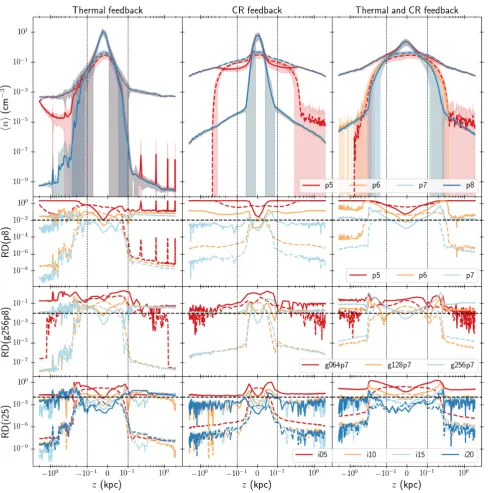
z above or below the disc. Examples of density profiles are shown in the top panel of Fig.1.
For each parameter of interest, we compare profiles for different parameter values with a reference model by com-puting the relative difference
RD(X, z) = 2
n(z)−nX(z) n(z) +nX(z)
, (1)
with X the parameter value that identifies the reference model. A model is considered sufficiently converged if the relative difference is of the level of 1 % or less for all values ofz.
We start with the number of iterations of our algorithm that is needed to obtain converged densities. The bottom row of Fig.1shows the relative difference between the den-sity profiles after 5, 10, 15 and 20 iterations, and the ref-erence result after 25 iterations. The largest diffref-erences be-tween the low iteration number models and the reference model are located near the central disc. The ionised disc between 0.5 and 2 kpc is converged to 1 % accuracy after 20 iterations, which is the number we will use for all our simulations.
Table 1.Naming convention for the convergence tests and source model parameter exploration.
simulation name number of iterations grid resolution number of photon packets
Ci20g128p7 20 128×128×256 107
Ci05g128p7 5 128×128×256 107
Ci10g128p7 10 128×128×256 107
Ci15g128p7 15 128×128×256 107
Ci25g128p7 25 128×128×256 107
Ci20g064p7 20 64×64×128 107
Ci20g256p7 20 256×256×512 107
Ci20g256p8 20 256×256×512 108
Ci20g128p5 20 128×128×256 105
Ci20g128p6 20 128×128×256 106
Ci20g128p8 20 128×128×256 108
simulation name random seed ionising luminosity scale height (s−1source−1) (pc)
Ir42l49s063 42 4.26×1049 63.0
Ir19l49s063 19 4.26×1049 63.0
Ir55l49s063 55 4.26×1049 63.0
Ir42l48s063 42 4.26×1048 63.0
Ir42l50s063 42 4.26×1050 63.0
Ir42l49s032 42 4.26×1049 31.5
Ir42l49s126 42 4.26×1049 126.0
number of photon packets used to discretize the stellar ra-diation field. If this number is too low, discretization error will dominate our simulation, and the radiation field will be unable to spread throughout the simulation box. The top rows of Fig.1show the average densities for different num-bers of photon packets, and for a fixed grid resolution of 128×128×256 cells. It is immediately clear that the re-sults for the simulations with only 105 photon packets are qualitatively different from those of the other simulations, illustrating how the radiation field is unable to efficiently ionise the box if too few photon packets are used. Just as in the case of the number of iterations, using a low number of photons also affects the scale height of the ionised disc. The relative difference drops below 1 % for the simulations with 107 photon packets, and this is the number that we will use in consecutive simulations.
A last important parameter for the convergence of our models is the grid resolution. Unlike the number of itera-tions or photon packets, this parameter is not immediately linked to our photoionisation algorithm. This means that we can obtain a converged photoionisation solution for any given grid resolution by using enough photon packets and iterations. If the grid samples the density field very badly, then this solution will not be converged to the solution im-posed by the underlying density field, but from the point of view of the photoionisation algorithm, it will be converged nonetheless. Conversely, parameters that lead to a converged result for one grid resolution, will not necessarily work for another resolution. The central row of Fig.1shows how us-ing a 256×256×512 grid with only 107photon packets seems
to change our result, indicating that we need at least this resolution to obtain a converged result. However, if we
re-run the same model with 10 times more photon packets, then the solution looks much more similar to the 128×128×256 result, showing that the latter resolution is sufficient for con-vergence. This is to be expected, as this is the resolution used byGirichidis et al.(2016b), so we are effectively overresolv-ing the input density field with a 256×256×512 grid. As pointed out byde Avillez & Breitschwerdt(2004);Hill et al.
(2012), this resolution does not guarantee converged density fields in the midplane of the SILCC simulations, and might cause us to overestimate the ionising luminosity necessary to ionise the extended disc.
We conclude that 20 iterations of our algorithm, using a grid of 128×128×256 cells and 107 photon packets, is
sufficient to obtain converged vertical density profiles for the ionised disc.
3.2 Ionising source model
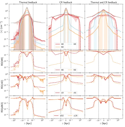
Before we can discuss the effect of changing the source lu-minosity or scale height of the source distribution on our re-sults, we need to quantify the scatter introduced by our sam-pling of the source distribution. To this end, we rerun each of our models with two different seeds for the random gen-erator that generates the positions of our discrete sources.
Figure 1. Top row :average neutral (full line) and ionised (dotted line) density for a given number of photon packets used in our algorithm. The shaded regions represent the scatter within slices of equal height above the disc. For clarity, the region close to the midplane has been plotted on a linear scale, while the outer regions are plotted on a logarithmic scale. The dashed vertical lines indicate the transition from the linear to the logarithmic region. Note that the large scatter near the midplane causes some of the shaded regions to have negative lower bounds, which can not be represented on the logarithmic scale.Other rows :relative difference between the average densities of the indicated models and the reference model for different model parameters:top :number of photon packets,middle :grid resolution,bottom :number of iterations. The dashed horizontal lines represent the target 1 % convergence limit.
positions of the sources can enhance asymmetries present in the density field. However, for the ionised gas density, and especially the extended disc which is of most interest to us, the relative differences between different source models are small. We conclude that the overall structure of our solution is independent of the numerical details of our ionising source
model, so that we can use a single realization of the source model to study the structure of the ionised disc.
Figure 2.Top row :average neutral (full line) and ionised (dotted line) density for a given ionising luminosity per ionising source. The shaded regions represent the scatter within slices of equal height above the disc. For clarity, the region close to the midplane has been plotted on a linear scale, while the outer regions are plotted on a logarithmic scale. The dashed vertical lines indicate the transition from the linear to the logarithmic region. Note that the large scatter near the midplane causes some of the shaded regions to have negative lower bounds, which can not be represented on the logarithmic scale.Bottom rows :relative difference between the average densities of the indicated models and the reference model for different model parameters:top :ionising luminosity per source,middle :random seed used to generate source positions,bottom :scale height of the ionising disc.
which we do not resolve. To address this uncertainty, we run models with different ionising luminosities per ionising source. The top rows of Fig.2show the density profiles for three different values of the luminosity : the generic value of 4.26×1049s−1, a value that is 10 times lower, and a value
that is 10 times higher. The latter is not really physical, but it is instructive to see how it affects our results.
up with an extended neutral disc instead of an ionised disc. However, when the luminosity is high enough, an ionised disc is created, the structure of which is relatively independent of the total ionising luminosity. Just as with the different random seeds above, we see that a different luminosity has some effect on the width of the central density profile, but does not really affect the extended disc (provided the lu-minosity is high enough to ionise it). The neutral density profile is affected, but only in the regions where the neutral gas fraction is already quite low.
The bottom row of Fig.2shows the relative differences for models with different values for the ionising source dis-tribution scale height : the generic value of 63 pc, a value which is half of that, and a value which is twice the generic value. It is clear that the scale height of the sources has a small effect on the value of the neutral fraction, as it is easier for hard ionizing radiation to escape from the dense inner disc if the source distribution is more extended.
We conclude that the extended ionised disc in our models is robust against changes in our ionising source model, provided that the ionising luminosity of the combined sources is sufficient to ionise the disc. These results are in agreement with previous results ofWoodet al.(2010).
3.3 Time evolution
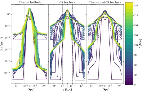
Fig.3shows the build-up of the density profiles over time, by post processing snapshots at a 10 Myr interval from time 0 Myr to the final snapshot at 250 Myr we extensively dis-cussed before, for each of the three feedback models. For the model with only thermal feedback, the profiles quickly reach a stable configuration in less than 50 Myr, for the models with cosmic ray feedback, the build-up is slower and it takes approximately 100 Myr to reach a stable disc.
The figure also shows how all three models at first have very low disc densities, which slowly increase over time. For the model with only thermal feedback, this increase is lim-ited, while for the other two models the disc growth is more extended.
It is important to note that these results were obtained in post processing, so there is no dynamical effect of the ionizing radiation on the evolution of the simulation model (other than the feedback model employed by the SILCC sim-ulations themselves). Furthermore, all our results used the same source model, independent of the evolution of the un-derlying SILCC model.
3.4 Emission lines
To calculate emission lines, we used the full version of CMa-cIonize, which treats the temperature of the ISM as a
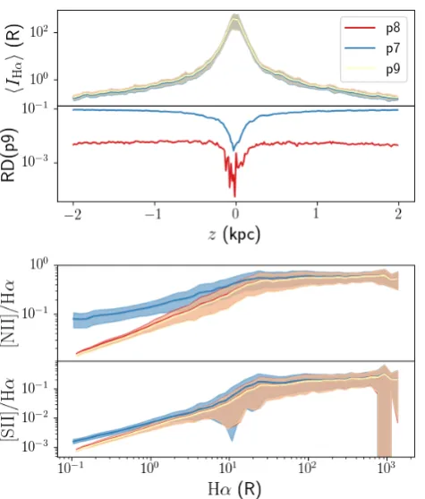
vari-able rather than a constant, and uses heating and cool-ing terms to obtain a converged temperature and ionisation state for each cell in the grid. Since the abundances of most coolants are significantly lower than those of hydrogen and helium, we increased the number of photons for these simu-lations with a factor of 10 to get better signal to noise ratios for the coolant ionic fractions. The convergence of the result-ing Hαprofiles and forbidden line emission ratios is shown in Fig.4 for the model with both thermal and cosmic ray feedback. We see that 108 photon packets is sufficient to get converged Hαprofiles and emission line ratios.
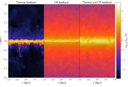
Fig.5shows simulated maps of the Hαintensity for our different models. It is clear that the Hα emission is signif-icantly more extended in the simulations including cosmic ray feedback. Note that the Hαintensities we find here are significantly higher than those found byBarnes et al.(2014) (see Section 3.4.2 below).
Fig. 6 shows horizontally averaged Hα profiles. It is clear that the simulation with only thermal feedback has very low intensities at even moderate heights above the mid-plane, which indicates that this model does not have an ex-tended ionized disc. By fitting an exponential profile of the form Hα(z) = Hα0exp(−|z|/zs) at heights above and below
500 pc for the models with cosmic ray feedback, we can de-termine the Hαscale heightzsfor those models. This yields
values of 0.643 kpc and 0.659 kpc for the model with only cosmic ray feedback, and 0.674 kpc and 0.723 kpc for the model with both thermal and cosmic ray feedback. These values are in line with observed Hαscale heights in the Milky Way, which range from∼100 pc in the inner galaxy ( Mad-sen & Reynolds 2005), over∼400 pc in the near spiral arms (Haffner, Reynolds & Tufte 1999; Hill et al.2014; Krish-narao et al. 2017) and values of∼700 pc in the local so-lar neighbourhood (Gaensler et al.2008;Savage & Wakker 2009), to values of more than 1 kpc in the far Carina arm (Krishnarao et al. 2017). The values we find are also sig-nificantly higher than the∼ 200 pc scale heights found in
Barnes et al.(2014).
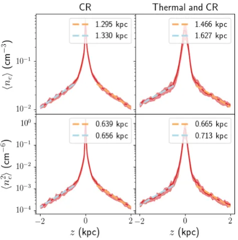
Gaensler et al. (2008) propose to measure the fill-ing factor of ionized gas by comparfill-ing Hα scale heights with electron scale heights obtained from pulsar disper-sion measurements. Assuming an ionizing gas filling factor which is constant as a function of height, the electron scale heightzs,ne (which traces the electron densityne) and Hα
scale heightzs,n2
e (which scales as n
2
e) should be linked by zs,ne/zs,n2
e = 2. However, if these scale heights are inferred
from integrated quantities, then the presence of neutral re-gions in the integral could skew this ratio to higher values for low altitudes. We test this for our simulations by fitting scale heights tone(z) andn2e(z), as shown in Fig.7. As can
be seen, thezs,n2
e values we find are in good agreement with
the integrated Hαvalues. Furthermore, thezs,ne values we
find are consistent with a ratio of 2.
When we look at emission line ratios, the corre-spondence between model and observations is much less favourable however. Fig.8shows the [NII]/Hαand [SII]/Hα
Figure 3.Average neutral (full line) and ionised (dotted line) density profile at different times during the simulations. For clarity, the region close to the midplane has been plotted on a linear scale, while the outer regions are plotted on a logarithmic scale. The dashed vertical lines indicate the transition from the linear to the logarithmic region.
3.4.1 Cosmic ray heating
One possible source of heating would be heating by cosmic rays. The cosmic ray model employed by the SILCC simula-tions introduces an extra pressure term and associated adi-abatic heating and cooling due to cosmic rays, but does not constitute a direct heating term (Girichidis et al.2016b). This means we cannot directly use the simulation snapshots to provide us with the required additional heating. We know however that cosmic rays can directly transfer energy to the gas by the generation of dampened Alfv´en waves (Wentzel 1971), a process which scales with n−e1/2, where ne is the
electron density in the gas (Wiener, Zweibel & Oh 2013). To test if cosmic ray heating can explain the observed line ratios, we run additional photoionisation simulations with the advanced model that treats both the ionisation balance and the temperature as a variable, and include an extra heating term that scales withn−e1/2:
Hcr=
1.2×10⁻²⁷erg cm−9/2s−1Ccrn−e1/2e
−|z|/hcr, (2)
where Ccr is a constant parameter of our model, z is the
height above the disc,hcr is the scale height of the cosmic
ray heating, and the numerical factor was based on the fac-tor given in Wiener, Zweibel & Oh (2013). As in Wiener,
Zweibel & Oh(2013), we choose a value hcr = 1.333 kpc.
We will consider different values of the parameterCcr.
We also implemented a second cosmic ray heating scheme that is based on the more exact expression for the cosmic ray heating(Wiener, Zweibel & Oh 2013):
Hcr=vA.∇Pcr, (3)
where vA is the Alfv´en speed (vA = √ B
µ0mpne, with B
the magnetic field,µ0 the vacuum permeability andmpthe
proton mass), and Pcr is the cosmic ray pressure (Pcr =
(γcr−1)ecr, withγcr= 4/3 the cosmic ray polytropic index,
andecrthe cosmic ray energy density).Bandecrare present
in the SILCC outputs, so our alternative heating term then can be formulated as
Hcr=
1.2×10⁻²⁷erg cm−9/2s−1Ccr0
B.∇ecr √
ne
, (4)
withCcr0 a constant parameter. This heating term will be
trivially zero for the SILCC model without cosmic ray feed-back.
Figure 4.Top :Hαintensity profiles as a function of height and relative difference for simulation with three different values of the photon packet number: 107(p7), 108(p8) and 109(p9).Bottom : line ratios for the same simulations.
electron density is low due to the high neutral fraction of the gas. We therefore, before entering the complex temperature iteration for a cell, compute the neutral fraction at a fixed temperature of 8000 K for that cell. If the cell has a neutral fraction that is higher than a cut off value of 0.75, we assume the cell is fully neutral and set its temperature to 500 K. In this case we do not enter the detailed cooling and heating routine, and avoid problems with finding the neutral fraction in cells with high densities and low electron densities.
Similarly, we also need to take care when heating the cells to very high temperatures, as we only included the rel-evant heating and cooling processes up to temperatures of about 30,000 K. We therefore manually reset the tempera-ture to 30,000 K if cosmic ray heating pushes it to higher values.
Fig. 9 shows the temperature profiles for various strengths of the cosmic ray heating. It is clear that cos-mic ray heating is able to push the average temperature to higher values. However, it is also worth noting that a significant fraction of the gas ends up at 30,000 K, the im-posed temperature limit, especially for cells at higher al-titudes above the disc. These cells will have very low Hα
intensities, so they do not contribute significantly to the ob-served line ratios. Fig.10shows the hot gas filling factor in each horizontal slice of the simulation, defined as the frac-tion of the 128×128 cells in the slice with a temperature of 30,000 K. For comparison, we also show the hot gas filling factor in the actual SILCC snapshots. It is clear that the
models with high cosmic ray feedback contain a lot of cells with very high temperatures. To reproduce the hot gas filling factor of the SILCC simulations in the models with cosmic ray feedback, we would need a cosmic ray heating parameter with about 10% of the value advocated inWiener, Zweibel & Oh(2013), or the more advanced cosmic ray heating model with the highest parameter value.
Note that both cosmic ray heating models produce sim-ilar results. As can be seen from the bottom panel of Fig.9, both mechanisms predominantly heat low density ionised gas, and cause a sharp increase in temperature at a density threshold set by the value of the heating parameter.
Also note that gas with densities lower than ∼
10−2 cm−3 will most likely be shock heated and ionised to
temperatures>105K, an effect that we did not incorporate in our post-processing treatment. Therefore, we find that all but the strongest cosmic ray heating realisations only heat gas that would already be heated by other physical mecha-nisms.
Finally, Fig. 8 shows the line ratios for the different cosmic ray heating models. It is clear that the cosmic ray heating does not affect the high Hα intensity end of the curve, which corresponds to radiation emitted by the central disc. Cosmic ray heating does affect the low intensity line ratios in the diffuse ionised disc, and effectively changes the sign of the slope of the curve, leading to a trend that is more in line with the observed trend, although the effect is only noticeable for high values of the cosmic ray heating factor. This seems to indicate that the cosmic ray heating does not affect the temperature of the intermediate density ionised gas which is responsible for the observed Hαemission.
3.4.2 Lower total luminosity
We require a relatively high luminosity to ionise out to large scale heights, compared to the values that were used by
Barnes et al.(2014). This leads to Hαluminosities that are high compared to observed Hαluminosities. It is instructive to see how the temperature and line ratios change if a lower luminosity is used.
To this end, we run a set of simulations with the full version of the code, using lower luminosities for the ionising sources: a version with an ionizing luminosity of 4.26×1048s−1per ionising source (10% of the generic value),
and a version with a luminosity of 1.065×1049s−1per ion-ising source (25% of the generic value).
The results of these simulations are shown in Fig.11. As expected, the lower luminosities lead to more noisy tem-perature and Hαprofiles, as the sources are no longer able to ionise the entire low density disc. However, for the SILCC models including cosmic ray feedback, the Hαscale height for the simulation with 25% of the total ionizing luminosity is still comparable to the full luminosity result (as can be seen from Table2), and hence in line with observed scale heights in the Milky Way. Furthermore, the runs with lower intensity show a clear increase in temperature for interme-diate density ionised gas, which in turns translates into line ratios that increase with decreasing Hαintensity.
spec-Figure 5.Hαintensity maps for the three models att= 250 Myr. The Hαintensity is given in Rayleighs (R); 1 R corresponds to a column emissivity of 106photons cm−2 s−1 sr−1.
Table 2. Scale height of the Hα disc for the simulations with lower total ionising luminosities.
ionising luminosity scale heightz <0 scale heightz >0
(s−1 source−1) (kpc) (kpc)
TH1 CR0
4.26×1049 0.931 2.064
1.065×1049 0.964 2.065
4.26×1048 0.980 2.077
TH0 CR1
4.26×1049 0.659 0.643
1.065×1049 0.662 0.641
4.26×1048 0.352 0.051
TH1 CR1
4.26×1049 0.723 0.674
1.065×1049 0.204 0.585
4.26×1048 0.055 0.056
trum for large scale heights (Wood & Mathis 2004) : low fre-quency photons are preferentially absorbed at low heights, so that the spectrum that reaches higher heights contains relatively more high frequency hydrogen ionising photons, which heat the gas to higher temperatures. If the total
ion-ising luminosity is high, the fraction of photons absorbed at low heights will be low, and the hardening of the spectrum will happen over a large scale. However, if the luminosity is just enough to ionise out to the boundary of the simulation box, we see the full hardening of the spectrum and result-ing rise in temperature, while still keepresult-ing the gas ionised. There is however some fine tuning required: decreasing the total luminosity further to 10% of the generic value signif-icantly decreases the Hα scale length, and leads to results that are no longer in line with observations.
4 CONCLUSION
[image:10.595.41.279.528.712.2]Figure 6. Hα intensity profiles as a function of height for the three feedback models. The shaded regions show the scatter within planar regions of equal scale height. The dashed lines show exponential fits to the part of the curve with |z|>500 pc (we fitted the parts below and above the disc separately). The scale heights derived from these fits are indicated in the legend. The black dashed line indicates the sensitivity limit for the Wisconsin HαMapper (WHAM), a representative instrument used to ob-serve emission lines in the Milky Way disc. Note that the large scatter near the midplane causes some of the shaded regions to have negative lower bounds, which can not be represented on the logarithmic scale.
Figure 7.Average electron densityne(top) and squared electron densityn2
e (bottom) as a function of height above the disc. The red line shows the average value within slices of equal height, the shaded region shows the scatter within each slice. The dashed lines indicate exponential fits to the part of the curve with
|z|>500 pc (we fitted the parts below and above the disc sepa-rately). The scale heights derived from these fits are indicated in the legend.
However, most of our simulations are unable to repro-duce observed nitrogen and sulphur line ratios, even when additional heating due to cosmic rays is included in the model, since these models only affect the temperature of low density ionised gas that does not contribute to observed line ratios. Only if we use a total ionising luminosity that is marginally sufficient to ionise the DIG, we are able to in-crease the temperature of intermediate density ionised gas and reproduce observed Milky Way line ratios. This fine tun-ing can have several explanations:
• The ionising radiation itself is partially responsible for setting the scale height of the ionised gas. This would nat-urally lead to a correlation between the total ionising lumi-nosity and the scale height. However, we cannot study this effect in this work, as there is no direct dynamical link be-tween the SILCC simulations and our post-processing tool. We plan to repeat our analysis for thePeters et al.(2017) simulations that do include photoionization feedback.
• There is another physical heating mechanism that is re-sponsible for the extra heating that is necessary to explain observed line ratios, and that affects intermediate rather than low density ionised gas. In this case we would not need to fine tune the ionising luminosity.
• The dense gas surrounding young O stars aborbs about 75% of the ionising radiation from the star, so that only 25% is left to ionise the more diffuse surrounding gas. As we do not resolve the densest gas, this is an effect that is likely. But to find more accurate values of the ionising escape fraction, more detailed simulations of star forming clouds are necessary.
We hence have no satisfactory explanation for the ob-served line ratios in the DIG of the Milky Way, and leave this for future work. We do find that the observed decreasing line ratios of nitrogen and sulphur with increasing Hα inten-sity are not necessarily explained by an increasing average ISM temperature with increasing scale height, as is often assumed. Instead, these line ratios could also be consistent with an increase in temperature dispersion with increasing scale height, with an overall constant or decreasing average temperature.
ACKNOWLEDGEMENTS
We want to thank the anonymous referee for constructive and insightful remarks that significantly improved the qual-ity of this work. BV and KW acknowledge support from STFC grant ST/M001296/1. PG acknowledges support from the DFG Priority Program 1573 Physics of the Interstel-lar Medium as well as funding from the European Research Council under ERC-CoG grant CRAGSMAN-646955.
REFERENCES
Barnes, J. E., Wood, K., Hill, A. S., Haffner, L. M., 2014, MN-RAS, 440, 3027
Berkhuijsen, E. M., Fletcher, A., 2008, MNRAS, 390, L19 Daflon, S., Cunha, K., de la Reze, R., Holtzman, J., Chiappini,
C., 2009, AJ, 138, 1577
[image:11.595.48.286.428.668.2]Figure 8.Line ratios for the simulations with and without cosmic ray heating. The different lines correspond to different values of the cosmic ray heating factorsCcr or Ccr0 , as indicated in the legend. The blue line corresponds to the line ratios of the reference model without cosmic ray heating. All values have been binned in 50 logarithmically spaced bins. The shaded regions show the scatter within the bins. The black dashed line is the WHAM sensitivity limit, while the blue dots represent observational data from the WHAM survey (Haffner, Reynolds & Tufte 1999). Note that the large scatter for some Hαintensities causes the shaded regions to have negative lower bounds, which can not be represented on the logarithmic scale.
Elmegreen, B. G., 1997, ApJ, 477, 196
Gaensler, B. M., Madsen, G. J., Chatterjee, S., Mao, S. A., 2008, Publ. Astron. Soc. Australia, 25, 184
Garmany, C. D., Conti, P. S., Chiosi, C., 1982, ApJ, 263, 777 Gatto, A., Walch, S., Naab, T., Girichidis, P., W¨unsch, R., Glover,
S. C. O., Klessen, R. S., Clark, P. C., Peters, T., Derigs, D., Baczynski, C., Puls, J., 2017, MNRAS, 466, 1903
Girichidis, P., Walch, S., Naab, T., Gatto, A., W¨unsch, R., Glover, S. C. O., Klessen, R. S. , Clark, P. C., Peters, T., Derigs, D., Baczynski, C., 2016a, MNRAS, 456, 3432
Girichidis, P., Naab, T., Walch, S., Hanasz, M., Mac Low, M.-M., Ostriker, J. P., Gatto, A., Peters, T., W¨unsch, R., Glover, S. C. O., Klessen, R. S., Clark, P. C., Baczynski, C., 2016b, ApJL, 816, L19
Haffner, L. M., Reynolds, R. J., Tufte, S. L., 1999, ApJ, 523, 223 Haffner, L. M., Dettmar, R.-J., Beckman, J. E., Wood, K., Slaving, J. D., Giammanco, C., Madsen, G. J., Zurita, A., Reynolds, R. J., 2009, Rev. Mod. Phys., 81, 969
Hill, A. S., Benjamin, R. A., Kowal, G., Reynolds, R. J., Haffner, L. M., Lazarian, A., 2008, ApJ, 686, 363
Hill, A. S., Joung, M. R., Mac Low, M.-M., Benjamin, R. A., Haffner, L. M., Klingenberg, C., Waagan, K., 2012, ApJ, 750, 104
Hill, A. S., Benjamin, R. A., Haffner, L. M., Gostisha, M. C.,
Barger, K. A., 2014, ApJ, 787, 106 Jenkins, E. B., 2009, ApJ, 700, 1299
Krishnarao, D., Haffner, L. M., Benjamin, R. A., Hill, A. S., Barger, K. A., 2017, ApJ, 838, 43
Madsen, G. J., Reynolds, R. J., 2005, ApJ, 630, 925 Ma´ız-Apell´aniz, J., 2001, AJ, 121, 2737
Mathis, J. S., 2000, ApJ, 544, 347
Nakanishi, H., Sofue, Y., 2003, PASJ, 55, 191
Pauldrach, A. W. A., Hoffmann, T. L., Lennon, M., 2001, A&A, 375, 161
Peters, T., Naab, T., Walch, S., Glover, S. C. O., Girichidis, P., Pellegrini, E., Klessen, R. S., W¨unsch, R., Gatto, A., Baczyn-ski, C., 2017, MNRAS, 466, 3239
Reynolds, R. J., 1990, ApJ, 348, 153
Reynolds, R. J., Haffner, L. M., Tufte, S. L., 1999, ApJL, 525, L21
Savage, B. D., Wakker, B. P., 2009, ApJ, 702, 1472
Simpson, J. P., Rubin, R. H., Colgan, S. W. J., Erickson, E. F., Haas, M. R., 2004, ApJ, 611, 338
Sternberg, A., Hoffmann, T. L., Pauldrach, A. W. A., 2003, ApJ, 599, 1333
Figure 9.Top :average temperature profiles for the simulations with and without cosmic ray feedback. The coloured lines are the results for different values of the cosmic ray heating factorsCcr orC0cr, as indicated in the legend. The blue line Ccr = 0 is the reference model without cosmic ray heating. The shaded regions show the scatter within slices of equal scale height.Bottom : tem-perature as a function of ionised density for the same simulations. The results have been binned in 50 logarithmically spaced bins; the shaded regions represent the scatter within the bins. The ver-tical dashed lines represent the density threshold below which the gas will likely be shock heated, an effect which we do not take into account in our treatment.
D., Baczynski, C., 2015, MNRAS, 454, 238 Wentzel, D. G., 1971, ApJ, 163, 503
Wiener, J., Zweibel, E. G., Oh, S. P., 2013, ApJ, 767, 87 Wood, K., Mathis, J. S., 2004, MNRAS, 353, 1126
Wood, K., Mathis, J. S., Ercolano, B., 2004, MNRAS, 348, 1337 Wood, K., Haffner, L. M., Reynolds, R. J, Mathis, J. S., Madsen,
G., 2005, ApJ, 633, 295
Wood, K., Hill, A. S., Joung, M. R., Mac Low, M.-M., Benjamin, R. A., Haffner, L. M., Reynolds, R. J., Madsen, G. J., 2010, ApJ, 721, 1397
This paper has been typeset from a TEX/LATEX file prepared by the author.
[image:13.595.314.546.107.262.2]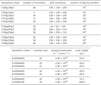


![Figure 11. Average temperature and Hα intensity as a function of height above the disc, temperature as a function of ionised density,and [NII]/Hα and [SII]/Hα line strenghts as a function of Hα intensity for the models with different values for the total io](https://thumb-us.123doks.com/thumbv2/123dok_us/8999151.396711/14.595.52.539.105.678/average-temperature-intensity-temperature-strenghts-function-intensity-dierent.webp)
