Very low mass stars and brown dwarfs in Upper Scorpius using Gaia DR1 : mass function, disks, and kinematics

VERY LOW-MASS STARS AND BROWN DWARFS IN UPPER SCORPIUS USING GAIA DR1: MASS FUNCTION, DISKS AND KINEMATICS

Neil J. Cook,1, 2 Aleks Scholz,3 andRay Jayawardhana2

1_{Institut de Recherche sur les Exoplan`etes, Universit´e de Montr´eal, Montr´eal, QC, Canada, H3T 1J4} 2_{Faculty of Science, York University, 4700 Keele Street, Toronto, Canada, ON M3J 1P3}

3_{SUPA, School of Physics & Astronomy, University of St. Andrews, North Haugh, St. Andrews, KY16 9SS, UK}

(Received September 11, 2017; Revised October 16, 2017; Accepted October 17, 2017)

Submitted to AJ

ABSTRACT

Our understanding of the brown dwarf population in star forming regions is dependent on knowing distances and proper motions, and therefore will be improved through theGaiaspace mission. In this paper, we select new samples of very low mass objects (VLMOs) in Upper Scorpius using UKIDSS colors and optimised proper motions calculated using Gaia DR1. The scatter in proper motions from VLMOs in Upper Scorpius is now (for the first time) dominated by the kinematic spread of the region itself, not by the positional uncertainties. With age and mass estimates updated using Gaia parallaxes for early type stars in the same region, we determine masses for all VLMOs. Our final most complete sample includes 453 VLMOs of which∼125 are expected to be brown dwarfs. The cleanest sample is comprised of 131 VLMOs, with∼105 brown dwarfs. We also compile a joint sample from the literature which includes 415 VLMOs, out of which 152 are likely brown dwarfs. The disc fraction among low-mass brown dwarfs (M <0.05M) is substantially higher than in more massive objects, indicating that discs around mass brown dwarfs survive longer than in low-mass stars overall. The low-mass function for 0.01 < M < 0.1M is consistent with the Kroupa IMF. We investigate the possibility that some ‘proper motion outliers’ have undergone a dynamical ejection early in their evolution. Our analysis shows that the color-magnitude cuts used when selecting samples introduce strong bias into the population statistics due to varying level of contamination and completeness.

Keywords: brown dwarfs — stars: lowmass — stars: mass function — open clusters and associations: individual: Upper Sco

Corresponding author: Neil J. Cook

[email protected]

2 _{Cook et al.}

1. INTRODUCTION

Most newly formed stars have masses significantly lower than the Sun. The characteristic mass of star formation, the peak of the Initial Mass Function (IMF), is around 0.2M, almost independent of environment (Bonnell et al.

2007). The mass distribution of objects formed in young clusters extends far below the sub-stellar limit at 0.08M and into the planetary (fusion-less) mass domain at<0.015M (Luhman 2012; Scholz et al. 2012). In this very low mass (VLM) domain, a variety of formation channels might play a role, including turbulent fragmentation of clouds, dynamical ejections from multiple systems, or disc fragmentation (seeWhitworth et al. 2007).

Very low mass object (VLMOs) are also viable host stars for exoplanet systems, as evidenced by discoveries of Earth-sized or -massed planets around mid M dwarfs (Berta-Thompson et al. 2015; Anglada-Escud´e et al. 2016;Dittmann et al. 2017;Gillon et al. 2017). The ubiquity of these systems poses an interesting challenge for core accretion theories, as discs around young objects in this mass domain usually do not seem to have sufficient material to form these type of systems (Scholz et al. 2006; Testi et al. 2015; Pascucci et al. 2016), implying very rapid formation. VLMOs are also possible hosts of ultracool dwarfs with L, T, or Y spectral types (Bardalez Gagliuffi et al. 2013;Cook et al. 2016,

2017).

Identifying and characterizing the VLM population in star forming regions provides the observational constraints on star formation scenarios as well as the samples for in-situ studies of planet formation. Traditionally, the selection of VLM cluster members is based on cuts in color-magnitude and proper motion space, followed by spectroscopy to confirm (Luhman et al. 2003; Wilking et al. 2004; Scholz et al. 2012). So far, proper motion cuts were limited to a few nearby regions with space motions significantly offset from the Galactic background. The output from the astrometry missionGaia is about to change that (Gaia Collaboration et al. 2016a,b). It is anticipated that the final Gaia data releases will provide the first large, uniform sample of parallaxes for young brown dwarfs in addition to sub-milliarcsecond precision in proper motions.

Gaia published its first data release in 2017 (Gaia Collaboration et al. 2016a,b, henceforth Gaia DR1). While Gaia DR1 does not yet provide Gaia-internal parallaxes and has not yet reached optimum astrometric precision, it can already be used for improving current selection methods for young VLMOs and to refine the resulting samples, as we demonstrate in this paper for the nearest OB association Upper Scorpius. Using the combined parallaxes from the Tycho-Gaia Astrometric Solution (TGAS) for bright young stars, the estimates for distances, age and spatial depth for nearby star forming regions can be solidified. With the help of the Gaia DR1 astrometry, the scatter in proper motions from VLMOS in Upper Scorpius is now (for the first time) dominated by the kinematic spread of the region itself, not by the positional uncertainties. For this particular region later data releases are unlikely to significantly improve the member selection from proper motions. Upper Scorpius is a region mostly free from reddening, therefore follow-up spectroscopy is not as essential here as in other star forming regions.

In this paper, we estimate distance, age and spatial depth from higher-mass Upper Scorpius members (Section2). We establish new samples of VLM members of Upper Scorpius using photometry from the United Kingdom Infrared Digital Sky Survey Galactic Clusters Survey (UKIDSS/GCS, Lawrence et al. 2007, see Section 3), and optimized astrometry obtained by combining Gaia DR1 with other catalogs (Section 4). Using these new samples we estimate masses (Section 5.1), test the the disc fraction as a function of mass (Section 5.2) and the mass function (Section

5.3). We also make a first attempt at tracking down kinematic outliers (Section5.4), i.e. objects with proper motions significantly different from their nearby siblings, which could be those who experienced an early dynamical ejection from a disc. The paper is intended to pave the way for future studies of other star forming regions based on the next Gaia data releases.

For the purposes of this paper, we use the term VLMO for all objects with masses below_.0.2M, including very low mass stars, brown dwarfs and planetary mass objects.

2. THE UPPER SCORPIUS ASSOCIATION WITH GAIA DR1

When deriving stellar properties for members of star forming regions, the main source of uncertainty are distance and age. Gaia DR1 does not provide parallaxes for very low mass members of Upper Scorpius – this is expected to be included in later data releases – but the TGAS catalog does contain parallaxes for a substantial sample of early-type stellar members. TGAS1_{, is a combination of the Tycho-2 with the Gaia catalog, listing astrometric data for ∼2.5}

25

20

15

10

5

0

Proper motion in Right Ascension direction [mas yr

_]

40

35

30

25

20

15

10

5

0

Pr

op

er

m

ot

ion

in

D

ec

lin

at

ion

[m

as

yr

1

]

4

5

6

7

8

9

10

Parallax [mas]

0.0

2.5

5.0

7.5

10.0

12.5

15.0

17.5

20.0

Number of objects

230

235

240

245

250

255

260

Right Ascension [deg]

40

35

30

25

20

15

10

De

cli

na

tio

n

[d

eg

]

0.2

0.0

0.2

0.4

0.6

0.8

1.0

1.2

B V

0

1

2

3

4

5

6

M

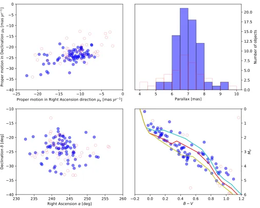
Figure 1. The 74 higher-mass members of Upper Scorpius used to determine distance, age and spatial depth for Upper Scorpius (in blue). The upper left panel shows their distribution in proper motion, the upper right panel shows their distance spread, the bottom left panel shows the distribution in space, and the lower right panel shows the color-magnitude diagram with 7, 10, and 15M yrisochrones2_{(cyan, red, yellow) fromSiess et al.(2000). Over-plotted in red are the rejected candidates.}

million stars (Michalik et al. 2014; Gaia Collaboration et al. 2016a,b). In this section we aim to use this dataset to re-determine distance and age for Upper Scorpius .

We start with the sample of high-mass members of Upper Scorpius fromde Zeeuw et al.(1999), selected as a moving group using Hipparcos astrometry. The mean Hipparcos distance in this sample is 145±1 pc. From the 120 members listed there, 85 have an entry in TGAS (with 100matching radius). From the catalog of primarily K-type members byPecaut et al. (2012), we add 36 stars without Hipparcos, but with TGAS entry. To clean the sample, we remove objects with parallax error>10% (16 objects), without Tycho-2 photometry (4 objects) or magnitude error>0.1 mag (24 objects), and with implausible distances>200 pc (9 objects) leaving 74 objects (47 objects rejected in total, taking into account those rejected by multiple criteria).

Five of the rejected stars at distance>200 pc are classified as K-M giants in the Michigan Spectral Survey (Houk & Smith-Moore 1988), among them HIP83542, also rejected byPecaut et al. (2012). In Figure1, the cleaned sample has clusters around (−11.7,−24.2) masyr−1_{, with standard deviation of 3 masyr}−1_.

4 _{Cook et al.}

Arenou et al. (2017). The parallax error translates to a median distance error of 7.8 pc and a √N scaled error of ±0.9 pc for the distance of the association. Thus, this provisional distance estimate from TGAS is within the error bars of the Hipparcos result. The parallax distribution (see Figure 1, upper right panel) has a standard deviation of 15.2 pc. Subtracting the errors in quadrature, this suggests a depth of the region along the line of sight of about ±13 pc. For comparison, in the plane of the sky, the sample is contained within an area of 20 deg diameter in both RA and DEC, corresponding to 50 pc at the distance of Upper Scorpius .

From the cleaned sample, we produce a color-magnitude diagram (see Figure 1, lower right panel). The absolute magnitudes have been calculated using the individual TGAS distances for each star, eliminating the error caused by the depth of the region. Uncertainties inMv andB−V are comparable to the size of the symbols for most objects.

Variability is expected to have a minor effect on the position of the stars in the diagram for a region of this age. Without widespread accretion or discs (Luhman 2012), the only plausible source of variability is magnetic activity, which typically does not cause large amplitudes, even at this young age (Grankin et al. 2008). Therefore, the spread in the color-magnitude diagram likely corresponds to a real age spread in Upper Scorpius .

Over-plotted in Figure1 are the 7, 10, and 15M yrisochrones2 _{(cyan, red, yellow) fromSiess et al. (2000), using} a metallicity of Z = 0.02 (solar metallicity,Siess et al. 2000) and the Kenyon & Hartmann (1995) conversion table. These three isochrones bracket most of the sample for (B−V)<0.8. For later-type objects the spread in the data points exceeds the model dispersion, partly due to increased photometric errors. Thus 7-15M yris a plausible minimum estimate for the age spread in this region. This is consistent with recent age studies for Upper Scorpius , seePecaut & Mamajek (2016); Fang et al.(2017), but in conflict with earlier claims of 5±2M yrbyPreibisch et al.(2002). Note that we checked isochrones with non-solar metallicity and the differences were negligible for our purposes.

3. VERY LOW MASS OBJECTS IN UPPER SCORPIUS

Many previous works have studied the population of VLMOs in Upper Scorpius (e.g.Slesnick et al. 2008; Dawson et al. 2011;Lodieu et al. 2011;Luhman & Mamajek 2012;Dawson et al. 2013;Lodieu 2013;Lodieu et al. 2013;Dawson et al. 2014). Most use various color cuts to select potential VLMOs, and use proper motions (either calculated or obtained from large catalogs) to identify candidates moving in a similar way to known Upper Scorpius members. One of the main uncertainties of membership (when distance is unknown) is the uncertainties associated with the calculated proper motions. Thus more precise proper motions tend to lead to identifying a better sample of VLMOs in Upper Scorpius .

In this section we compile two samples, the first is a sample directly taken from the literature (and thus based on various colors cuts and slightly different selection criteria), henceforth the ‘L-sample’, the second is a large uniform sample, based on the initial color selection fromLodieu(2013), henceforth the ‘C-sample’.

3.1. The L-sample

Although there are many surveys that study Upper Scorpius , we decided to choose those surveys that identify VLMO members using UKIDSS GCS (Lawrence et al. 2007) or similar (i.e. VISTA) photometry so that we had sub-samples that had Z, Y, J, H, K photometry (’L-ZYJHK sample’); or had H and K photometry (‘L-HK only sample’). We combined data from Dawson et al. (2011), Lodieu et al. (2011), Dawson et al. (2013), Lodieu(2013), Lodieu et al.

(2013), andDawson et al.(2014) to obtain a sample of 789 unique objects, of which 493 were in the L-ZYJHK sample and 295 were in the L-HK only sample using photometry from both UKIDSS GCS DR10 (henceforth DR10) and the GCS Science verification release (henceforth SV;Dye et al. 2006). Tables 7 and 8 give the full detail on how many objects were in each source catalog.

3.2. The C-sample

The data for the C-sample were obtained using the WFCAM Science Archive (WSAHambly et al. 2008)3_{using SQL} queries (see Appendix B). We followed the initial sampling used by Lodieu(2013), using identical bright saturation limits, limiting merged passband selection to 100_{and retaining only point-like, non-duplicated sources. We decided to} also follow the sub-sample selection ofLodieu(2013), defining samples that had Z, Y, J, H, K photometry (’C-ZYJHK sample’); or as having H and K photometry (‘C-HK only sample’). We obtained 2,653,897 sources for the C-ZYJHK

2

1.0

1.5

2.0

2.5

3.0

Z-J

12

14

16

18

20

22

Z

1

2

3

4

5

Z-K

12

14

16

18

20

22

Z

0.0

0.5

1.0

1.5

2.0

2.5

3.0

3.5

H-K

10

12

14

16

18

H

0.4

0.6

0.8

1.0

1.2

1.4

1.6

1.8

Y-J

12

14

16

18

20

Y

1.0

1.5

2.0

2.5

3.0

J-K

10

12

14

16

18

20

J

Cut lines

From SQL query

Dawson et al. 2011

Lodieu et al. 2011

Dawson et al. 2013

Lodieu 2013a ZYJHK DR10

Lodieu 2013a ZYJHK DR10 R

Lodieu 2013a ZYJHK SV

Lodieu 2013a HK Only

Lodieu et al. 2013b

Dawson et al. 2014

1.5

2.0

2.5

3.0

3.5

4.0

4.5

5.0

Z-K

1.0

1.5

2.0

2.5

3.0

J-K

6 _{Cook et al.}

sample from DR10, 157,325 sources for the C-ZYJHK sample from SV, and 7,473,530 for the ‘HK sample’ of which 4,814,722 do not have Z, Y and J photometry (i.e. the C-HK only sample).

FollowingLodieu(2013) we split the C-ZYJHK sample into a sub-sample affected by reddening and a sub-sample not affected by reddening (henceforth denoted asRfor the reddened sample), and remove those objects with ‘HK extinction’ in the C-HK only sample (see table 1 from Lodieu 2013). The C-ZYJHK DR10 sample had 1,722,423 sources flagged as not affected by reddening and 931,474 flagged as being affected by reddening. The C-ZYJHK SV sample had no sources flagged as affected by reddening. The C-HK only sample had 3,652,715 that were not removed due to reddening.

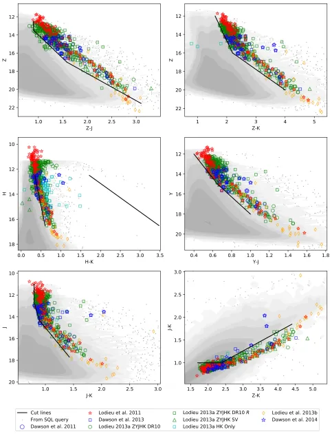
To select VLMOs from the full samples we used the literature sample and the color cuts identified byLodieu(2013). Our final color cuts are nearly identical toLodieu(2013) except that we add an additional cut toH−K, this was in order to make sure our samples were not affected by the tail of the giant branch (See the H againstH−K plot in Figure2). The cuts are listed below.

ZZJ cut =



  

  

Z−J >0.90 12.50< Z <13.50

Z <5.14(Z−J) + 8.86 13.50< Z <17.00

Z <3.00(Z−J) + 12.25 17.00< Z <21.55

HHK cut =







H <15.38(H−K) + 7.23 12.50< H <16.50

H >2.28(H−K) + 8.58 12.50< H <16.50

JJK cut =



  

  

J−K >0.80 11.00< J <12.70

J <17.00(J−K)−0.90 12.70< J <14.35

J <6.33(J−K)−8.67 14.35< J <17.70

ZZK cut =







Z <6.67(Z−K) + 1.33 12.00< Z <16.00

Z <2.22(Z−K) + 11.11 16.00< H <20.00

YYJ cut =







Y <12.00(Y −J) + 7.20 12.00< Y <15.00

Y <8.57(Y −J) + 9.43 15.00< Y <18.00

JKZK cut =







(J−K)<1.00 1.70<(Z−K)<2.40

(J−K)<0.42(Z−K) 2.40<(Z−K)<4.40

We decided to keep two different combinations of these cuts to see the effect they had on the final population selected, the first used all the above cuts (denoted by a HK ) and the second used all the color cuts except the ‘HHK cut’.

Thus we have samples with ‘C-ZYJHK DR10’, ‘C-ZYJHK DR10R’, ‘C-ZYJHK DR10 HK ’, ‘C-ZYJHK DR10R HK ’, ‘C-ZYJHK SV’, ‘C-ZYJHK SV HK ’, and ‘C-HK only’ (where the ‘C’ distinguishes the sub-samples from the L-samples described in Section3.1). The number of objects left after the color cuts are shown in Table 1and a full break down of numbers is presented in tables7 and8.

3.3. Discussion of sub-samples

Table 1.The results for the C-samples after the color cuts are applied.

Sample Total before cuts ZZJ HHK JJK ZZK YYJ JKZK Total after cuts

C-ZYJHK DR10 1,722,423 5,654 - 23,134 9,977 12,122 245,810 1,305

C-ZYJHK DR10

R

931,474 1,538 - 9,940 2,569 5,824 400,451 811

C-ZYJHK SV 157,325 135 - 887 143 206 29,723 86

C-ZYJHK DR10

HK

1,722,423 5,654 2,359 23,134 9,977 12,122 245,810 66

C-ZYJHK DR10

RHK

931,474 1,538 318 9,940 2,569 5,824 400,451 77

C-ZYJHK SV HK 157,325 135 71 887 143 206 29,723 33

C-HK only 3,652,715 - 1,526 - - - - 1,526

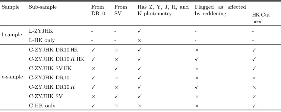
Table 2. The definition of the samples

Sample Sub-sample From

DR10

From SV

Has Z, Y, J, H, and K photometry

Flagged as affected

by reddening _{HK Cut}

used

l-sample L-ZYJHK - - X -

-L-HK only - - × -

-c-sample

C-ZYJHK DR10 HK X × X × X

C-ZYJHK DR10R HK X × X X X

C-ZYJHK SV HK × X X × X

C-ZYJHK DR10 X × X × ×

C-ZYJHK DR10R X × X X ×

C-ZYJHK SV × X X × ×

C-HK only X × × × X

flagged as having reddening (R). We do this so we can analyze the affect different cuts have on our results. Table2

describes these sample subsets and their differences.

Each of our sub-samples has specific properties due to the imposed selection criteria. The C-HK only sample is going to be the least well defined sample due to the lack of Z, Y and J photometry and therefore lack of all the color cuts except the HK cut. The Rsamples (i.e. C-ZYJHK DR10 Rand C-ZYJHK DR10RHK ) are expected to be more contaminated due to the increased reddening those source experience (i.e. reddened objects will be scattered across the color cuts). The SV samples (i.e. C-ZYJHK SV and C-ZYJHK SV HK ) rely on science verification photometry and will be less complete than the DR10 samples. The SV samples also cover a slightly different spatial location than the DR10 samples and thus may have slight differences in age (see the age gradient from figure 9 of Pecaut & Mamajek 2016). The L-sample consists of some higher mass objects (due to the lack of, for example, brightness cuts), however due to some of these objects being spectroscopically confirmed we do not further reduce the L-sample and use it for comparative purposes only.

8 _{Cook et al.}

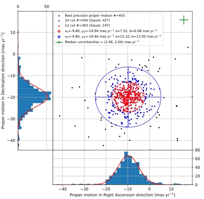
Best precision proper motion #=493 2 cut #=440 (Gauss: 427) 1 cut #=303 (Gauss: 197)

x0=-9.80, y0=-19.94 mas yr 1 a=7.55, b=6.98 mas yr 1 x0=-9.80, y0=-19.94 mas yr 1 a=15.10, b=13.95 mas yr 1

Median uncertainties = (2.06, 2.09) mas yr 1

0

50

40

30

20

10

0

10

Pr

op

er

m

ot

ion

in

D

ec

lin

at

ion

d

ire

cti

on

[m

as

yr

1

]

40

30

20

10

0

10

Proper motion in Right Ascension direction [mas yr

_]

0

20

40

60

80

Figure 3. Proper motion vector diagram showing the one and two sigma ellipses used to define Upper Scorpius membership for the L-ZYJHK sample (for the best precision proper motions). The numbers of objects found were compared to a two-dimensional Gaussian distribution of equal center and covariance. Median uncertainties are shown in the upper right corner.

hand, the C-ZYJHK DR10 should be the most complete. Throughout this paper we do all analysis on all samples to check how much of an effect selection has on any results we obtain.

4. PROPER MOTION ANALYSIS

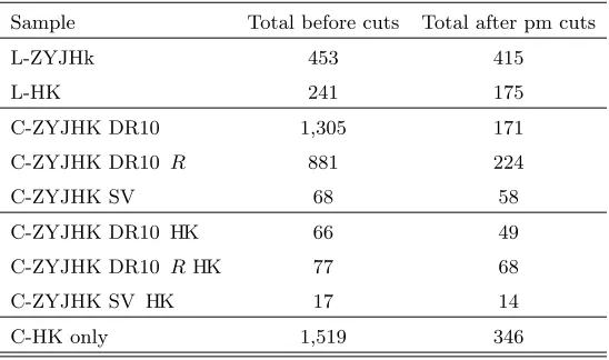
Table 3. The result of the Upper Scorpius membership selection.

Sample Total before cuts Total after pm cuts

L-ZYJHk 453 415

L-HK 241 175

C-ZYJHK DR10 1,305 171

C-ZYJHK DR10 R 881 224

C-ZYJHK SV 68 58

C-ZYJHK DR10 HK 66 49

C-ZYJHK DR10 RHK 77 68

C-ZYJHK SV HK 17 14

C-HK only 1,519 346

these proper motions the most precise total proper motion was selected for each object (where total proper motion and associated uncertainty are defined in Equation1).

µT otal=

q

µ2

α+µ2δ σµT otal =

1

µT otal

q

(σµαµα) 2_{+ (σ}

µδµδ)

2 ₍₁₎

where µα is the proper motion component in the Right Ascension direction (cos(δ)) and µδ is the proper motion

component in the Declination direction.

We decided to exclude PPMXL proper motions as no sources with only PPMXL proper motions had uncertainties better than∼10 masyr−1. The stars that had a suitable proper motion measurement 716 out of 789 for the L-sample, all 2259 C-ZYJHK DR10 objects, 68 out of 86 C-ZYJHK SV objects, all 17 C-ZYJHK SV HK , 1,519 out of 1,526 C-HK only sample (see tables7and8 for a full break down of numbers).

Our uncertainties in proper motion are sufficiently small that we do not need to select members based on a proper motion uncertainty circle (this is in contrast to previous studies where large uncertainties dominate the velocity dispersion of Upper Scorpius ). However, since the proper motion of Upper Scorpius is very small, we decided to use the L-sample to define a two-sigma membership ellipse for Upper Scorpius (such that we avoid an overlap with (µα, µδ) = (0.0,0.0) masyr−1). We compared the median and standard deviations for the L-ZYJHK, L-HK only

and the combined sample. The L-ZYJHK sample was found to have a center of (µα, µδ)=(-9.80, -19.94) masyr−1,

with standard deviations of (µα, µδ)=(7.51, 6.96) masyr−1. The L-HK only sample was found to have a center of

(µα, µδ)=(-7.78, -18.39) masyr−1, with standard deviations of (µα, µδ)=(7.82, 9.14) masyr−1. The combined

L-sample was found to have a center of (µα, µδ)=(-9.04, -19.46) masyr−1, with standard deviations of (µα, µδ)=(7.88,

8.08) masyr−1_.

We thus chose to define candidate members of Upper Scorpius as those within an ellipse of center (µα, µδ)=(-9.80,

-19.94) and x and y radii of (µα, µδ)=(15.10, 13.95) masyr−1(defined from the L-ZYJHK distribution). This was

then used to select members from the L-sample and C-sample. We keep 415/453 and 175/241 of those objects from the L-ZYJHK and L-HK only samples respectively. For the C-ZYJHK DR10Rsample we kept in 224/881 candidates, and 68/77 C-ZYJHK DR10R HK candidates. For the C-ZYJHK sample we identified 171/1,305 candidates, and for the C-ZYJHK HK sample we kept 49/66 candidates. For the C-ZYJHK SV sample we identify 58/68 as Upper Scor-pius candidates, and 14/17 for the C-ZYJHK SV HK sample. The C-HK only sample resulted in 346/1,519 candidates being identified. These numbers are summarized in Table 3 and tables 7 and 8 have a full break down of numbers. Figure3 shows the L-ZYJHK sample used to selected candidates from both the L-samples and the C-samples.

10 _{Cook et al.}

10000

12000

14000

16000

18000

20000

22000

Wavelength [Å]

7.5

8.0

8.5

9.0

9.5

10.0

Absolute magnitude [mags]

Age = 8.0 Myrs, Mass=0.03 M , Teff=2699.0 K, L=-2.29 L , log(g)=3.88 , Radius=0.329 R , Li/L0=1.0

Age = 10.0 Myrs, Mass=0.04 M , Teff=2768.0 K, L=-2.35 L , log(g)=4.11 , Radius=0.292 R , Li/L0=1.0

Age = 15.0 Myrs, Mass=0.06 M , Teff=2892.0 K, L=-2.3 L , log(g)=4.32 , Radius=0.282 R , Li/L0=1.0

Age = 8.0 Myrs

Age = 10.0 Myrs

Age = 15.0 Myrs

Data

Z

Y

J

H

K

nid00003

Figure 4. Example isochronal fit for L-sample object UGCS J161625.98-211222.9. Fit gives a mass of 0.04+0−0..0201M.

5. PROPERTIES OF VLMOS IN UPPER SCORPIUS

With an estimated age of 10M yr(with a spread between 7 and 15M yr) and assuming a distance of∼145 pc (with a spread of±13 pc, Section2) it is possible to estimate mass and luminosity by fitting the photometry to theoretical isochrones. We use the 8, 10 and 15M yrBaraffe et al.(2015) isochrones (BHAC15) to give a lower, median and upper bound to each of our objects with UKIDSS Z, Y, J, H and K photometry (i.e. we only fit sources which have all five photometric magnitudes), we choose 8M yras the lower bound as the 7M yrisochrone is not computed for BHAC15. In this section we describe the fitting process and use these, withWide-Field Infrared Survey Explorer(WISE,Wright et al. 2010) data to infer a disc fraction, analyze the mass distributions and explore the proper motion distribution of our candidates.

5.1. Isochronal fitting

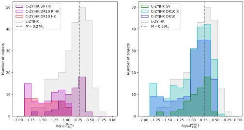
2.00 1.75 1.50 1.25 1.00 0.75 0.50 0.25 0.00

log

1M

)

0

10

20

30

40

50

Number of objects

C-ZYJHK SV HK

C-ZYJHK DR10 R HK

C-ZYJHK DR10 HK

L-ZYJHK

M = 0.2M

2.00 1.75 1.50 1.25 1.00 0.75 0.50 0.25 0.00

log

1M

)

0

10

20

30

40

50

Number of objects

C-ZYJHK SV

C-ZYJHK DR10 R

C-ZYJHK DR10

L-ZYJHK

M = 0.2M

Figure 5. Log mass histogram for the C-sample using the HK cut (left) as compared to cases without (right). The HK cut effectively constrains the mass of the objects to∼0.2M(black vertical line) whereas without the HK cut the masses extend to

higher mass objects. Over-plotted, in both sub-plots for reference, is the L-sample (with no HK cut applied).

The mass estimate attached to each age (8, 10 and 15 M yr) were then combined, giving an expected value, an upper and a lower uncertainty (described in Equation2).

M= (Mmedian)+σMupper −σM_lower

Mmedian= median fit Mlower = lower fit Mupper= upper fit

σMlower =



     

     

Mupper− Mmedian ifMlower= 0 andMupper6= 0

Mupper− Mmedian ifMlower<0 andMupper<0

Mmedian ifMlower=Mupper= 0

Mmedian− Mlower else-wise

σMupper =



     

     

Mmedian− Mlower ifMlower= 0 andMupper6= 0

Mmedian− Mlower ifMlower<0 andMupper<0

Mmedian ifMlower=Mupper= 0

Mupper− Mmedian else-wise

(2)

where M is the mass estimate associated with the best fit (lower, median and upper bounding) model. This gave us appropriate uncertainties for the estimated mass based on the spread in ages found for Upper Scorpius (Section

12 _{Cook et al.}

0.0

0.5

1.0

1.5

2.0

2.5

3.0

UKIDSS (Z J)

2

4

6

8

10

12

14

16

M

Z

Age = 4.0 Myr

Age = 5.0 Myr

Age = 8.0 Myr

Age = 10.0 Myr

Age = 15.0 Myr

Age = 20.0 Myr

Age = 25.0 Myr

Figure 6. Absolute Z magnitude against (Z-J) color (Hertzsprung-Russell diagram) for the L-sample. Objects with discs are marked with an orange star. Median uncertainties are shown with the green cross. The distribution is consistent with an average age of 10M yrand a spread from 8 to 15M yr.

The estimated mass distributions for the C-sample using the HK cut as compared to cases without can be seen in Figure 5 (with the L-sample over-plotted in both cases for comparison). From Figure5 the differences between the sub-samples becomes clear. The L-samples contain a significant number of higher-mass stars. The application of the HK cut (left panel compared to right panel) shows that this cut effectively removes objects of mass _. 0.2M and hence avoids contamination. The Hertzsprung-Russell diagram for the L-sample is shown in Figure6. The distribution of colors seems consistent with a typical age of 10 M yr.

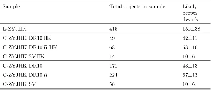
Defining brown dwarfs to have a mass less than 0.075Mwe calculated the number of our objects that are likely brown dwarfs (with the uncertainty coming from those that overlap in mass due to their mass estimate uncertainty). The L-ZYJHK sample was found to have 152±38 out of the 415 objects as likely brown dwarfs, the C-ZYJHK DR10 HK , C-ZYJHK DR10 R HK and C-ZYJHK SV HK samples were found to have 42±11, 53±10 and 10±6 respectively, and the C-ZYJHK DR10, C-ZYJHK DR10 Rand C-ZYJHK SV samples were found to have 48±13, 67±13 and 10±6 respectively. These numbers are presented in Table4. We note that the number of brown dwarfs are quite similar in the samples with and without the HK cut; in this mass domain the samples should avoid most contamination.

Table 4. Numbers of possible brown dwarfs (Mass less than 0.075M).

Sample Total objects in sample Likely

brown dwarfs

L-ZYJHK 415 152±38

C-ZYJHK DR10 HK 49 42±11

C-ZYJHK DR10RHK 68 53±10

C-ZYJHK SV HK 14 10±6

C-ZYJHK DR10 171 48±13

C-ZYJHK DR10R 224 67±13

C-ZYJHK SV 58 10±6

added to the flux due to the presence of a disc). For this reason we also fitted the masses using only ZYJ and ZYJH and flagged any objects which were identified as having possible discs (from Section 5.2). This led to having three mass estimates for each object and thus we were able to see any differences due to ‘bad’ H and K photometry. After comparing objects with possible discs to those without discs no discernible difference was seen, thus the mass estimates were not affected by those objects having discs. Most objects had a maximum variation (due to using different sets of photometry) of 0.01M thus we decided to retain our mass estimates using all five bands.

Our chi-squared minimization does not take into account the uncertainties in magnitude (shown on Figure4) and thus it does not take into account any uncertainty due to distance or spread in the association. Note that the spread in the association is significantly larger than the distance uncertainty on Upper Scorpius (145±2 pc), i.e.±13 pc from Section2, thus an additional uncertainty on the mass estimates will be introduced (this will be solved with later Gaia data releases giving distances to individual objects).

As a further sanity check for our mass estimates we compared our results to theLodieu et al.(2011) and Dawson et al. (2014) samples which both have spectroscopically confirmed members of Upper Scorpius . We compare the spectral types from the literature to the mass estimates from the isochrones and compare the mass estimates from the literature to the mass estimates from the isochrone fits (see Figure7). The figures show the expected trends and broad agreement, but there are also clear discrepancies. In the left panel of Figure7 some objects (with very low masses) have surprisingly early spectral types, Dawson et al. (2014) concluded that some of these objects might be further away than the rest of the objects identified as being part of Upper Scorpius . For these objects our mass estimate will be underestimated. In the right panel of Figure7 we find that our mass estimates are systematically higher (by ∼ 1σ) compared to Lodieu et al. (2011). That study derives masses by comparing bolometric magnitudes (derived from J-band) with NextGen/DUST models (Baraffe et al. 1998andChabrier et al. 2000respectively), using a distance consistent with ours, but assume an age of 5 Myr (priv. comm. Lodieu 2017). Between 5 and 10 Myr, VLMOs drop in luminosity, i.e. assuming a younger age leads to lower mass estimates.

5.2. Disc fraction as a function of mass

Using the (W1−W2) color excess cut and W3 excess cut from Dawson et al.(2013, shown in Equation3) we were able to identify possible discs in our candidate members.

W1W2 Disc =J <60(W1−W2)−9 W3 Disc =SN RW3>5 andW3<10

Disc = (W1W2 Disc) or (W3 Disc)

(3)

14 _{Cook et al.}

M2.0 M3.0 M4.0 M5.0 M6.0 M7.0 M8.0 M9.0 L0.0 L1.0 L2.0

Spectral type from literature

0.0

0.1

0.2

0.3

0.4

0.5

0.6

0.7

Es

tim

at

ed

m

as

s f

ro

m

is

oc

hr

on

e [

M

]

Lodieu+2011

Dawson+2014

0.0

0.1

0.2

0.3

0.4

0.5

0.6

0.7

Mass from literature [M ]

0.0

0.1

0.2

0.3

0.4

0.5

0.6

0.7

Es

tim

at

ed

m

as

s f

ro

m

is

oc

hr

on

e [

M

]

x=y

Lodieu+2011

Figure 7. The comparison between our mass estimates from the isochrones to those objects in Upper Scorpius with spectral type and masses from the literature (members with spectra) fromLodieu et al.(2011) andDawson et al. (2014).

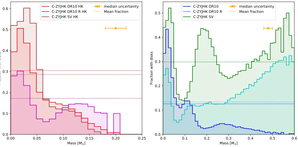
0.00 0.05 0.10 0.15 0.20 0.25

Mass [M ] 0.0

0.1 0.2 0.3 0.4 0.5 0.6

Fraction with disks

C-ZYJHK DR10 HK C-ZYJHK DR10 R HK C-ZYJHK SV HK

median uncertainty Mean fraction

0.0 0.1 0.2 0.3 0.4 0.5 0.6

Mass [M ] 0.0

0.1 0.2 0.3 0.4 0.5

Fraction with disks

C-ZYJHK DR10 C-ZYJHK DR10 R C-ZYJHK SV

median uncertainty Mean fraction

Figure 8. Disc fraction as a function of estimated mass (from isochrones). All samples were chosen to have 50 bins ranging from 0.0 to 0.6M(bin sizes were chosen to represent, approximately, the median uncertainty in mass estimates) and used 10,000

2.25 2.00 1.75 1.50 1.25 1.00 0.75 0.50 0.25

log10(Mass1M ) 2

3 4 5 6 7

log10

(d

N/

dM

)

C-ZYJHK DR10 HK C-ZYJHK DR10 R HK C-ZYJHK SV HK median uncertainty

2.25 2.00 1.75 1.50 1.25 1.00 0.75 0.50 0.25

log10(Mass1M ) 2

3 4 5 6 7

log10

(d

N/

dM

)

C-ZYJHK DR10 C-ZYJHK DR10 R C-ZYJHK SV median uncertainty

Figure 9. Mass functions (from isochrones). All samples were chosen to have 50 bins ranging from 0.0 to 0.6M(bin sizes were

chosen to represent, approximately, the median uncertainty in mass estimates) and used 10,000 samples in our Monte-Carlo analysis (see Section 5.2) for those objects with mass estimates. The dashed lines show the best fits to a mass function (α1 for 0.08< M <0.5M,α2 forM <0.08M), whereαis allowed to vary and the solid lines show the Kroupa mass function

(α= 1.3 for 0.08< M <0.5M,α= 0.3 forM <0.08M). All fits are scaled arbitrarily.

Table 5. The disc fractions found for the Upper Scorpius objects with WISE photometry.

Sample Number of objects

with discs

Number of objects in sample

Disc fraction

L-ZYJHK 47 244 19.3±2.5%

C-ZYJHK DR10 HK 14 46 30.4±6.8%

C-ZYJHK DR10RHK 11 64 17.2±4.7%

C-ZYJHK SV HK 4 14 28.6±12.1%

C-ZYJHK DR10 21 167 12.6±2.6%

C-ZYJHK DR10R 29 217 13.4±2.3%

C-ZYJHK SV 17 57 29.8±6.1%

29.8±6.1%), all fractions are presented in Table5. Combined these give a weighted mean disc fraction of 16.8±1.7%. All uncertainties are calculated as one-sigma uncertainties assuming binomial statistics (see tables 7 and8 for a full break down of numbers). This value is broadly consistent with previously published disc fractions for VLM stars and brown dwarfs in this region (Jayawardhana et al. 2003;Scholz et al. 2007).

16 _{Cook et al.}

2 1 0 1 2

Excess in proper motion in right ascension [ ] 2

1 0 1 2

Ex

ce

ss

in

p

ro

pe

r m

ot

ion

in

d

ec

lin

at

ion

[

]

Non-outliers=43/49 Outliers=6/49 2 Circle

Expected from Gaussian = 7/49

Figure 10. Proper motion excess diagrams for the C-ZYJHK DR10 HK sample. Excess is defined in Equation4.

The disc fractions derived in that manner give two important insights. One is that the choice of the sample has a non-negligible effect on the outcome. This is particularly apparent from the right panel in Figure 8, which shows the sample without the HK cut. Based on our assessment of contamination of these samples (see Section3.3and Section

4 the disc fractions derived from these samples have to be treated with caution. Contamination by background red giants might increase the fraction of objects with infrared excess in these samples, while contamination by background dwarf stars would reduce it. The strong fluctuations of disc fraction as a function of mass seen in these samples will be caused primarily by the varying influence of these contaminating samples, rather than actual changes in the disc fraction of VLMOs in Upper Scorpius. Discrepancies on the brown dwarf disc fraction presented in the literature may to a large extent be caused by differences in sample selection.

Second, the clean samples with the HK cut do show that disc fractions within the sub-stellar domain increase with decreasing mass. This is seen in all three samples in the left panel of Figure 8. This trend was already stated in previous work, most notably by Luhman & Mamajek (2012). In our samples, the disc fraction for M <0.05Mis about 2-3 times larger than at 0.05< M <0.15M. This is solid evidence for disc lifetimes significantly exceeding 10M yrfor low-mass brown dwarfs, confirming previous claims based on smaller samples (Riaz et al. 2009).

5.3. Mass function

Using the same MCMC process as in Section5.2we worked out the total number of objects in each mass bin. The mass function was then calculated using the total number of objects in each mass bin divided by the size of the mass bin. Uncertainties in number are assumed to be √N, and the uncertainty on dM is assumed to be the size of the mass bin. This means the uncertainty ondN/dM is dominated by the uncertainty on the mass estimates. In Figure8

we plot the mass function with the median uncertainties shown in yellow and the mass functions fromKroupa(2001), α= 1.3 for 0.08< M <0.5M, α= 0.3 forM <0.08M, scaled arbitrarily to match our number of objects. Note thatN, and thusdN/dM, are 10,000 times higher than our samples due to the Monte-Carlo samples used.

Table 6. The number of outliers (those with excess greater than 2 sigma) compared to the number of expected outliers from a Gaussian distribution (again beyond 2 sigma).

Sample Total objects in sample Non-outliers Outliers Expected Outliers from Gaussian

L-ZYJHK 415 347 68 57

C-ZYJHK DR10 HK 49 43 6 7

C-ZYJHK DR10RHK 68 59 9 10

C-ZYJHK SV HK 14 10 4 2

C-ZYJHK DR10 171 134 37 22

C-ZYJHK DR10R 224 187 37 30

C-ZYJHK SV 58 44 14 8

or the faintness limit our data is consistent with the Kroupa IMF. A value of α∼ 0.4 is also in line with previous determinations of the IMF in this region, e.g. ,Lodieu et al.(2013) findα= 0.45±0.11.

The right panel in Figure8which shows the samples without the HK cut again illustrates the effects of contamination on the mass function. In particular, there is a consistent ‘bump’ in the mass function just above 0.1M, which is most likely introduced by background objects. Echoing our previous comments, we would like to caution using this selection method for candidate members to derive population statistics for M > 0.1M, unless comprehensive spectroscopic characterisation is carried out to confirm youth and membership.

5.4. Proper motion outliers

In this subsection we explore the possibility that some of the VLMOs in Upper Scorpius have a dynamic history that deviates from the bulk of the population, for example, because they experienced an ejection in the early stages of their evolution, which might have stopped in-fall and constrained the mass. Ejections like that are part of a number of proposed formation scenarios for sub-stellar objects (e.g. Whitworth et al. 2007).

To test for this possibility, we compare the proper motion for each target compared to its ten nearest neighbors (nearest in Right Ascension and Declination). An excess in proper motion was calculated for each object and is defined in Equation4.

Excess (µα) =

(µα)Target−(µα)NN

q

σ2

(µα)Target+σ 2 (µα)NN

Excess (µδ) =

(µδ)Target−(µδ)NN

q

σ2

(µδ)Target+σ 2 (µδ)NN

(4)

where (µα,δ)NN is the median of the ten nearest neighbor objects proper motion in the Right Ascension/Declination

direction, andσ(µα,δ)NNis the standard deviation of the ten nearest neighbor objects in the Right Ascension/Declination direction. Thus excess is in units of sigma, where a value of zero would equate to an object having a proper motion component exactly equivalent to that of it’s neighbors.

This allowed us to flag any candidates with excesses beyond 2 sigma (defined by a circle in proper motion space). For the L-ZYJHK and L-HK only sample we found 68/415 and 31/175 outlier in our Upper Scorpius candidates. For the C-ZYJHK DR10 HK , C-ZYJHK DR10R HK and C-ZYJHK SV HK samples we found 6/49, 9/68 and 4/14 outliers in our Upper Scorpius candidates. For the C-ZYJHK DR10, C-ZYJHK DR10Rand C-ZYJHK SVsamples we found 37/171, 37/224, 14/58 outliers in our Upper Scorpius candidates. Figure 10 shows the excess distribution in proper motion for two samples, with the 2 sigma circle drawn and outliers highlighted in red. The numbers are reported in Table6.

Comparing the number of outliers with the outliers expected from a Gaussian distribution (last column in Table

18 _{Cook et al.}

distinct from the bulk population in the same area. For samples without the HK cut, the number of outliers is again expected to be affected by contamination, as discussed throughout this paper. We note that a proper motion of 2 mas, currently the median uncertainty of our optimized proper motions, translates into a velocity in the plane of the sky of 1.3 kms−1, which is comparable with the typical velocity dispersion found in radial velocity surveys of young brown dwarfs (Joergens 2006). Ejection velocities may in some cases be significantly beyond that level (Stamatellos & Whitworth 2009,Li et al. 2015), i.e. the lack of proper motion outliers already provides useful limits for formation scenarios. This topic is an area where we expect future data releases from Gaia to provide improved constraints.

6. CONCLUDING REMARKS

TheGaiamission is a powerful new tool in understanding star forming regions due to its new and future astrometry. For the first time regions such as Upper Scorpius are no longer limited by the uncertainty on proper motion (and with future Gaia data releases unknown distances). As such we show that both age and mass estimates can be vastly improved, giving insight into the initial mass function and through published photometry from WISE, the disc fractions of these populations. However, we caution that future inferences on populations (such as for example, but in no way limited to, mass functions and disc fraction) will be very dependent on the selection criteria used. It may be that rigorous selection (i.e. via full spectroscopic analysis) is required to really identify bona fide VLMOs and brown dwarfs from background objects and other contamination. This is especially valid for regions where reddening is important, but also applies, as shown in this paper, to regions free from extinction. Despite this we find that our mass functions (at least between 0.01< M < 0.1M) are consistent with the Kroupa IMF, that the disc fraction among low-mass brown dwarfs (M < 0.05M) is substantially higher than in more massive objects. We note that proper motions from Gaia will give us an opportunity to detect objects that were dynamically ejected early on. If done correctly, with future Gaia data and full spectroscopic follow-up the potential for nearby star forming regions to advance our knowledge of low-mass, very-low mass and planetary mass objects is extremely exciting.

ACKNOWLEDGMENTS

We would like to thank the anonymous referee whose careful reading of this paper and excellent comments were very welcome. We would like to thank Ogyen Verhagen, former undergraduate student at the University in St Andrews, whose final year project results motivated parts of this work. This work was supported in part by NSERC grants to RJ. This work has made use of data from the European Space Agency (ESA) mission Gaia (https://www.cosmos.esa.

int/gaia), processed by theGaiaData Processing and Analysis Consortium (DPAC,https://www.cosmos.esa.int/

web/gaia/dpac/consortium). Funding for the DPAC has been provided by national institutions, in particular the

institutions participating in theGaiaMultilateral Agreement. Specifically we use Gaia DR1 data (Gaia Collaboration et al. 2016a, Gaia Collaboration et al. 2016b) with more details available fromArenou et al.(2017),Lindegren et al.

(2016),van Leeuwen et al.(2017),Carrasco et al.(2016) andEvans et al.(2017). We make use of data products from WISE (Wright et al. 2010), which is a joint project of the UCLA, and the JPL/CIT, funded by NASA. The UKIDSS project is defined in Lawrence et al. (2007). UKIDSS uses the UKIRT Wide Field Camera (WFCAM;Casali et al. 2007). The photometric system is described inHewett et al.(2006), and the calibration is described inHodgkin et al.

Software:

APPENDIX

A. SQL QUERIES

A.1. The ZYJHK Sample

ZYJHK sample query (Private communications with N. Lodieu see Lodieu 2013). This query returned 2,653,897 sources from UKIDSS DR10 and 157,325 sources from the UKIDSS SV.

/∗ S t a r t ∗/

SELECT

s o u r c e I D , ra , d e c , zAperMag3 , zAperMag3Err , yAperMag3 , yAperMag3Err , jAperMag3 , jAperMag3Err , hAperMag3 , hAperMag3Err , k 1AperMag3 , k 1AperMag3Err , muRa , muDec , sigMuRa , sigMuDec

FROM

g c s S o u r c e

WHERE

r a BETWEEN 2 3 2 . 0 AND 2 5 5 . 0

AND d e c BETWEEN −30.0 AND −15.0

/∗ B r i g h t s a t u r a t i o n c u t−o f f s ∗/

AND zaperMag3 > 1 1 . 3

AND yaperMag3 > 1 1 . 5

AND j a p e r M a g 3 > 1 1 . 0

AND haperMag3 > 1 1 . 3 0

AND k 1aperMag3 > 9 . 9 0

/∗ L i m i t merged p a s s b a n d s e l e c t i o n t o 1 a r c s e c ∗/

AND z X i BETWEEN −1.0 AND +1.0

AND yXi BETWEEN −1.0 AND +1.0

AND j X i BETWEEN −1.0 AND +1.0

AND hXi BETWEEN −1.0 AND +1.0

AND k 1 X i BETWEEN −1.0 AND +1.0

AND z Eta BETWEEN −1.0 AND +1.0

AND yEta BETWEEN −1.0 AND +1.0

AND j E t a BETWEEN −1.0 AND +1.0

AND hEta BETWEEN −1.0 AND +1.0

AND k 1 E t a BETWEEN −1.0 AND +1.0

AND ( j p p E r r B i t s < 1 3 1 0 7 2 )

AND ( h p p E r r B i t s < 1 3 1 0 7 2 )

AND ( k 1 p p E r r B i t s < 1 3 1 0 7 2 )

/∗ R e t a i n o n l y p o i n t−l i k e s o u r c e s ∗/

AND ( (

( ( z C l a s s BETWEEN−2AND −1) OR ( z C l a s s S t a t BETWEEN −3.0 AND + 3 . 0 ) )

AND

( ( y C l a s s BETWEEN−2AND −1) OR ( y C l a s s S t a t BETWEEN −3.0 AND + 3 . 0 ) )

AND

( ( j C l a s s BETWEEN−2AND −1) OR ( j C l a s s S t a t BETWEEN −3.0 AND + 3 . 0 ) )

AND

( ( h C l a s s BETWEEN−2AND −1) OR ( h C l a s s S t a t BETWEEN −3.0 AND + 3 . 0 ) )

AND

( ( k 1 C l a s s BETWEEN−2AND −1) OR ( k 1 C l a s s S t a t BETWEEN −3.0 AND + 3 . 0 ) ) )

OR m e r g e d C l a s s BETWEEN−2 AND−1 OR m e r g e d C l a s s S t a t BETWEEN −3.0 AND +3.0 )

/∗ R e t a i n o n l y t h e b e s t r e c o r d when d u p l i c a t e d i n an o v e r l a p r e g i o n ∗/

AND ( p r i O r S e c = 0 OR p r i O r S e c = f r a m e S e t I D )

/∗ End ∗/

A.2. The HK-only Sample

HK-only sample query (Private communications with N. Lodieu see Lodieu 2013). This query returned 7,473,530 sources from UKIDSS DR10.

/∗ S t a r t ∗/

SELECT

s o u r c e I D , ra , d e c , zAperMag3 , zAperMag3Err , yAperMag3 , yAperMag3Err , jAperMag3 , jAperMag3Err , hAperMag3 , hAperMag3Err , k 1AperMag3 , k 1AperMag3Err , muRa , muDec , sigMuRa , sigMuDec

FROM

g c s S o u r c e

WHERE

r a BETWEEN 2 3 2 . 0 AND 2 5 5 . 0

AND d e c BETWEEN −30.0 AND −15.0

20 _{Cook et al.}

AND ( zaperMag3 < −0.9 e 9 OR zaperMag3 > 1 1 . 3 )

AND ( yaperMag3 < −0.9 e 9 OR yaperMag3 > 1 1 . 5 )

AND ( j a p e r M a g 3 < −0.9 e 9 OR j a p e r M a g 3 > 1 1 . 0 )

AND haperMag3 > 1 1 . 3 0

AND k 1aperMag3 > 9 . 9 0

/∗ L i m i t merged p a s s b a n d s e l e c t i o n t o 1 a r c s e c ∗/

AND ( z X i BETWEEN −1.0 AND +1.0 OR z X i < −0.9 e 9 )

AND ( yXi BETWEEN −1.0 AND +1.0 OR yXi < −0.9 e 9 )

AND ( j X i BETWEEN −1.0 AND +1.0 OR j X i < −0.9 e 9 )

AND hXi BETWEEN −1.0 AND +1.0

AND k 1 X i BETWEEN −1.0 AND +1.0

AND ( zE ta BETWEEN −1.0 AND +1.0 OR z Eta < −0.9 e 9 )

AND ( yEta BETWEEN −1.0 AND +1.0 OR yEta < −0.9 e 9 )

AND ( j E t a BETWEEN −1.0 AND +1.0 OR j E t a < −0.9 e 9 )

AND hEta BETWEEN −1.0 AND +1.0

AND k 1 E t a BETWEEN −1.0 AND +1.0

AND ( h p p E r r B i t s < 1 3 1 0 7 2 )

AND ( k 1 p p E r r B i t s < 1 3 1 0 7 2 )

/∗ R e t a i n o n l y p o i n t−l i k e s o u r c e s ∗/

AND ( (

( ( z C l a s s BETWEEN−2AND −1) OR ( z C l a s s S t a t BETWEEN −3.0 AND + 3 . 0 ) OR ( z C l a s s = −9999) )

AND

( ( y C l a s s BETWEEN−2AND −1) OR ( y C l a s s S t a t BETWEEN −3.0 AND + 3 . 0 ) OR ( y C l a s s = −9999) )

AND

( ( j C l a s s BETWEEN−2AND −1) OR ( j C l a s s S t a t BETWEEN −3.0 AND + 3 . 0 ) OR ( j C l a s s = −9999) )

AND

( ( h C l a s s BETWEEN−2AND −1) OR ( h C l a s s S t a t BETWEEN −3.0 AND + 3 . 0 ) )

AND

( ( k 1 C l a s s BETWEEN−2AND −1) OR ( k 1 C l a s s S t a t BETWEEN −3.0 AND + 3 . 0 ) ) )

OR m e r g e d C l a s s BETWEEN−2 AND−1 OR m e r g e d C l a s s S t a t BETWEEN −3.0 AND +3.0 )

/∗ R e t a i n o n l y t h e b e s t r e c o r d when d u p l i c a t e d i n an o v e r l a p r e g i o n ∗/

AND ( p r i O r S e c = 0 OR p r i O r S e c = f r a m e S e t I D )

/∗ End ∗/

B. THE SAMPLES BY NUMBER

In tables7 and8 we show the source counts (i.e. the number of objects used from the original tables), the number of objects with proper motions in the HSOY, GPS1, UCAC, GCS, and PPMXL catalogs. We show the number of objects with a ‘most precise’ proper motion (in the ‘best pm’ column, i.e. the smallest uncertainty as chosen from the HSOY, GPS1, UCAC and GCS catalogs, see Section4). We show the source counts for those object that have WISE photometry, have a disc as indicated by the Dawson cuts (‘W1W2 disc’, ‘W3 disc’ and the combination of the two ‘disc’ column, see Section5.2). The ‘mass est.’ column describes whether we were able to find a isochronal model that fit the data (see Section5.1). The ‘USco’ column gives the number in each which conforms to our selection criteria for an Upper Scorpius member (see Section4) and the numbers of objects in Upper Scorpius with discs, with a isochronal mass estimate and with both a disc and a isochronal mass estimate are shown in the last three columns. Tables9and

T able 7. The source coun ts fo r the L-sample. F or the L-sample n um b ers are also p resen ted b y original literature source catalog and ho w man y sources are presen t in U K ID S S GCS DR10 and the UKIDSS GCS Science v erification data. T ables a v ailable online in mac hine readable format. Flag T otal HSO Y GPS1 UCA C GCS PPMXL b est pm WISE W1W2 Disc W3 Disc Disc mass est. USco USco+ disc USco+ Wise+ mass

e

st.

USco disc+ mass

22 _{Cook et al.} T able 8. The source coun ts for the C-sample. T ables a v ailable online in ma chine readable format. The C -sample with th e HK cut applied. Flag T otal HSO Y GPS1 UCA C GCS PPMXL b est pm WISE W1W2 Disc W3 Disc Disc mass est. USco USco+ disc USco+ Wise+ mass

e

st.

USco disc+ mass

est. C-ZYJHK DR10 H K 66 21 24 0 66 36 66 63 14 3 15 66 49 14 46 14 C-ZYJHK DR10 R H K 77 24 35 0 77 42 77 73 12 1 12 77 68 11 64 11 C-ZYJHK SV H K 17 12 14 0 17 15 17 17 5 0 5 17 14 4 14 4 C-ZYJHK T o-tal H K 160 5 7 73 0 1 60 93 160 153 31 4 32 160 131 29 124 29 C-HK onl y 1526 870 807 225 1526 1032 1519 1395 180 98 214 1526 346 88 331 88 The C -sample without the HK cut applied. Flag T otal HSO Y GPS1 UCA C GCS PPMXL b est pm WISE W1W2 Disc W3 Disc Disc mass est. USco USco+ disc USco+ Wise+ mass

e

st.

USco disc+ mass

Table 9. Column descriptions for C-sample tables for C-ZYJHK DR10, C-ZYJHK DR10R, C-ZYJHK

SV, C-ZYJHK DR10 HK , C-ZYJHK DR10RHK , and C-ZYJHK SV HK and tables are available online

in machine readable format.

Column Name Description Unit UCD

UID Unique identifier (1) · · · meta.id;meta.main RAdeg Right Ascension in decimal degrees (J2000) deg pos.eq.ra;meta.main DEdeg Declination in decimal degrees (J2000) deg pos.eq.dec;meta.main Zmag UKIDSS Z magnitude mag phot.mag;em.IR e Zmag uncertainty in Zmag mag stat.error;em.IR Ymag UKIDSS Y magnitude mag phot.mag;em.IR e Ymag uncertainty in Ymag mag stat.error;em.IR Jmag UKIDSS J magnitude mag phot.mag;em.IR.J e Jmag uncertainty in Jmag mag stat.error;em.IR.J Hmag UKIDSS H magnitude mag phot.mag;em.IR.H e Hmag uncertainty in Hmag mag stat.error;em.IR.H Kmag K magnitude mag phot.mag;em.IR.K e Kmag uncertainty in Kmag mag stat.error;em.IR.K pm Most precise proper motion mas/yr pos.pm e pm Uncertainty in pm mas/yr stat.error;pos.pm r pm Reference for pm (2) · · · meta.bib pmRA Most precise proper motion in RA mas/yr pos.pm;pos.eq.ra e pmRA Uncertainty in pmRA mas/yr stat.error;pos.pm;pos.eq.ra pmDE Most precise proper motion in DE mas/yr pos.pm;pos.eq.dec e pmDE Uncertainty in pmDE mas/yr stat.error;pos.pm;pos.eq.dec WISE Has WISE photometry (3) · · · code.meta Disk Flagged as having a disc (3) (4) · · · code.meta MassFit Bestχ2_{fit for mass solMass phys.mass} bMassFit Lower uncertainty bound in MassFit solMass stat.error;phys.mass BMassFit Upper uncertainty bound in MassFit solMass stat.error;phys.mass TeffFit Bestχ2fit for effective temperature K phys.temperature.effective bTeffFit Lower uncertainty bound in TeffFit K stat.error;phys.temperature.effective BTeffFit Upper uncertainty bound in TeffFit K stat.error;phys.temperature.effective LumFit Bestχ2fit for luminosity solLum phys.luminosity bLumFit Lower uncertainty bound in LumFit solLum stat.error;phys.luminosity BLumFit Upper uncertainty bound in LumFit solLum stat.error;phys.luminosity log(g)Fit Bestχ2_{fit for surface gravity [cm/s2] phys.gravity} blog(g)Fit Lower uncertainty bound in log(g)Fit [cm/s2] stat.error;phys.gravity Blog(g)Fit Upper uncertainty bound in log(g)Fit [cm/s2] stat.error;phys.gravity RadFit Bestχ2_{fit for radius solRad phys.size.radius} bRadFit Lower uncertainty bound in RadFit solRad stat.error;phys.size.radius BRadFit Upper uncertainty bound in RadFit solRad stat.error;phys.size.radius chilow Low fitχ2 _{· · · stat.fit.chi2} chimid Mid fitχ2 · · · stat.fit.chi2 chihi High fitχ2 · · · stat.fit.chi2 WiseAndMass Has WISE photometry and a mass estimate · · · meta.code sigExpmRA Sigma excess in pmRA · · · stat.value;pos.pm;pos.eq.ra sigExpmDE Sigma excess in pmDE · · · stat.value;pos.pm;pos.eq.dec fnpmout Not an outlier in pm; 2σ(3) · · · meta.code.member fpmout Is an outlier in pm; 2σ(3) · · · meta.code.member

24 _{Cook et al.}

Table 9(continued)

Column Name Description Unit UCD

1 Of this merged detection as assigned by merge algorithm. ID is unique over entire WSA via program ID prefix. 2 hsoy = Hot Stuff for One Year (HSOY) catalog (Altmann et al. 2017); gps1 = Gaia-PS1-SDSS (GPS1) catalog (Tian

et al. 2017); gcs = The UKIRT Infrared Deep Sky Survey (UKIDSS) catalog (Lawrence et al. 2007); and ucac = UCAC5: New Proper Motions Using Gaia DR1 catalog (Zacharias et al. 2017).

3 1 = True, 2 = False

4_{Dawson et al.(2013) WISE W1-W2 or WISE W3 disc.}

Table 10. Column descriptions for the L-sample tables (L-ZJYHK and L-HKonly). Tables available online in machine readable format.

Column Name Description Unit UCD

UID Unique ID from catalog creation · · · meta.id;meta.main RAdeg Right Ascension in decimal degrees (J2000) deg pos.eq.ra;meta.main DEdeg Declination in decimal degrees (J2000) deg pos.eq.dec;meta.main Coord Source of main coordinates · · · meta.bib Cat Catalog contained in (1) · · · meta.bib Zmag Most precise Z magnitude mag phot.mag;em.opt.Z r Zmag Reference for Zmag (1) · · · meta.bib e Zmag uncertainty in Zmag mag stat.error;em.opt.Z Ymag Most precise Y magnitude mag phot.mag;em.opt.Y r Ymag Reference for Ymag (1) · · · meta.bib e Ymag uncertainty in Ymag mag stat.error;em.opt.Y Jmag Most precise J magnitude mag phot.mag;em.IR.J r Jmag Reference for Jmag (1) · · · meta.bib e Jmag uncertainty in Jmag mag stat.error;phot.mag;em.IR.J Hmag Most precise H magnitude mag phot.mag;em.IR.H r Hmag Reference for Hmag (1) · · · meta.bib e Hmag uncertainty in Hmag mag stat.error;phot.mag;em.IR.H Kmag Most precise K magnitude mag phot.mag;em.IR.K r Kmag Reference for Kmag (1) · · · meta.bib e Kmag uncertainty in Kmag mag stat.error;phot.mag;em.IR.K SpTCat spt from source catalog · · · src.spType r SpTCat Reference for SpTcat (1) · · · meta.bib MassCat Mass from source catalog solMass phys.mass r MassCat Reference for MassCat (1) · · · meta.bib fZYJHK Flag whether source ahs valid ZYJHK photometry (2) · · · meta.code fHKonly Flag that source only has HK photometry (2) · · · meta.code pm Most precise proper motion mas/yr pos.pm e pm Uncertainty in pm mas/yr stat.error;pos.pm r pm Reference for pm (3) · · · meta.bib pmRA Most precise proper motion in RA mas/yr pos.pm;pos.eq.ra e pmRA Uncertainty in pmRA mas/yr stat.error;pos.pm;pos.eq.ra pmDE Most precise proper motion in DE mas/yr pos.pm;pos.eq.dec e pmDE Uncertainty in pmDE mas/yr stat.error;pos.pm;pos.eq.dec MassFit Bestχ2_{fit for mass solMass phys.mass} bMassFit Lower uncertainty bound in MassFit solMass stat.error;phys.mass

Table 10(continued)

Column Name Description Unit UCD

BMassFit Upper uncertainty bound in MassFit solMass stat.error;phys.mass TeffFit Bestχ2fit for effective temperature K phys.temperature.effective bTeffFit Lower uncertainty bound in TeffFit K stat.error;phys.temperature.effective BTeffFit Upper uncertainty bound in TeffFit K stat.error;phys.temperature.effective LumFit Bestχ2_{fit for luminosity solLum phys.luminosity} bLumFit Lower uncertainty bound in LumFit solLum stat.error;phys.luminosity BLumFit Upper uncertainty bound in LumFit solLum stat.error;phys.luminosity log(g)Fit Bestχ2_{fit for surface gravity [cm/s2] phys.gravity} blog(g)Fit Lower uncertainty bound in log(g)Fit [cm/s2] stat.error;phys.gravity Blog(g)Fit Upper uncertainty bound in log(g)Fit [cm/s2] stat.error;phys.gravity RadFit Bestχ2fit for radius solRad phys.size.radius eRadFitL Lower uncertainty bound in RadFit solRad stat.error;phys.size.radius eRadFitU Upper uncertainty bound in RadFit solRad stat.error;phys.size.radius chilow Low fitχ2 · · · stat.fit.chi2 chimid Mid fitχ2 · · · stat.fit.chi2 chihi High fitχ2 · · · stat.fit.chi2 Disk Flagged as having a disc (2) (4) · · · meta.code WiseAndMass Has WISE photometry and a mass estimate (2) · · · meta.code sigExpmRA Sigma excess in pmRA · · · stat.value;pos.pm;pos.eq.ra sigExpmDE Sigma excess in pmDE · · · stat.value;pos.pm;pos.eq.dec fnotPMout Not an outlier in pm; 2σ(2) · · · meta.code.member fPMout Is an outlier in pm; 2σ(2) · · · meta.code.member 1 GCSSV = from UKIDSS Science verification (Lawrence et al. 2007); GCSDR10 = from UKIDSS DR10 (Lawrence et al. 2007);

D11 = fromDawson et al.(2011)]; L11 = FromLodieu et al.(2011); D13 = fromDawson et al.(2013); L13a = fromLodieu (2013): L13a HK from HK sample, L13a ZYJHK SV from the ZYJHK UKIDSS Science verification sample,L13a ZYJHK red from the ZYJHK UKIDSS DR10 affected by reddening sample, L13a ZYJHK nored from the ZYJHK UKIDSS DR10 devoid of reddening sample; L13b = fromLodieu et al.(2013); D14 = fromDawson et al.(2014).

2 1 = True, 2 = False

3 hsoy = Hot Stuff for One Year (HSOY) catalog (Altmann et al. 2017); gps1 = Gaia-PS1-SDSS (GPS1) catalog (Tian et al. 2017); gcs = The UKIRT Infrared Deep Sky Survey (UKIDSS) catalog (Lawrence et al. 2007); and ucac = UCAC5: New Proper Motions Using Gaia DR1 catalog (Zacharias et al. 2017).

4 From isochrones (i.e have ZYJHKW1W2 photometry).

REFERENCES

Altmann, M., Roeser, S., Demleitner, M., Bastian, U., &

Schilbach, E. 2017, A&A, 600, L4

Anglada-Escud´e, G., Amado, P. J., Barnes, J., et al. 2016,

Nature, 536, 437

Arenou, F., Luri, X. fand Babusiaux, C., Fabricius, C.,

et al. 2017, A&A, 599, A50

Astropy Collaboration, Robitaille, T. P., Tollerud, E. J.,

et al. 2013, A&A, 558, A33

Baraffe, I., Chabrier, G., Allard, F., & Hauschildt, P. H.

1998, A&A, 337, 403

Baraffe, I., Homeier, D., Allard, F., & Chabrier, G. 2015,

A&A, 577, A42

Bardalez Gagliuffi, D. C., Burgasser, A. J., & Gelino, C. R.

2013, Mem. Soc. Astron. Italiana, 84, 1041

Barrett, P., Hunter, J., Miller, J. T., Hsu, J.-C., &

Greenfield, P. 2005, in Astronomical Society of the

Pacific Conference Series, Vol. 347, Astronomical Data Analysis Software and Systems XIV, ed. P. Shopbell,

M. Britton, & R. Ebert, 91

Berta-Thompson, Z. K., Irwin, J., Charbonneau, D., et al.

2015, Nature, 527, 204

Bonnell, I. A., Larson, R. B., & Zinnecker, H. 2007, Protostars and Planets V, 149

Carrasco, J. M., Evans, D. W., Montegriffo, P., et al. 2016,

A&A, 595, A7

Casali, M., Adamson, A., Alves de Oliveira, C., et al. 2007,

A&A, 467, 777

26 _{Cook et al.}

Chambers, K. C. 2011, in Bulletin of the American Astronomical Society, Vol. 43, American Astronomical Society Meeting Abstracts #218, 113.01

Cook, N. J., Pinfield, D. J., Marocco, F., et al. 2016, MNRAS, 457, 2192

—. 2017, MNRAS, 467, 5001

da Costa-Luis, C., L., S., Mary, H., et al. 2017, tqdm/tqdm: tqdm v4.19.1 stable, , , doi:10.5281/zenodo.1001783.

https://doi.org/10.5281/zenodo.1001783

Dawson, P., Scholz, A., & Ray, T. P. 2011, MNRAS, 418, 1231

Dawson, P., Scholz, A., Ray, T. P., et al. 2013, MNRAS, 429, 903

—. 2014, MNRAS, 442, 1586

de Zeeuw, P. T., Hoogerwerf, R., de Bruijne, J. H. J., Brown, A. G. A., & Blaauw, A. 1999, AJ, 117, 354 Dittmann, J. A., Irwin, J. M., Charbonneau, D., et al.

2017, Nature, 544, 333

Dye, S., Warren, S. J., Hambly, N. C., et al. 2006, MNRAS, 372, 1227

Evans, D. W., Riello, M., De Angeli, F., et al. 2017, A&A, 600, A51

Fang, Q., Herczeg, G. J., & Rizzuto, A. 2017, ApJ, 842, 123 Gaia Collaboration, Prusti, T., de Bruijne, J. H. J., et al.

2016a, A&A, 595, A1

Gaia Collaboration, Brown, A. G. A., Vallenari, A., et al. 2016b, A&A, 595, A2

Gillon, M., Triaud, A. H. M. J., Demory, B.-O., et al. 2017, Nature, 542, 456

Grankin, K. N., Bouvier, J., Herbst, W., & Melnikov, S. Y. 2008, A&A, 479, 827

Hambly, N. C., Collins, R. S., Cross, N. J. G., et al. 2008, MNRAS, 384, 637

Hewett, P. C., Warren, S. J., Leggett, S. K., & Hodgkin, S. T. 2006, MNRAS, 367, 454

Hodgkin, S. T., Irwin, M. J., Hewett, P. C., & Warren, S. J. 2009, MNRAS, 394, 675

Houk, N., & Smith-Moore, M. 1988, Michigan Catalogue of Two-dimensional Spectral Types for the HD Stars. Volume 4, Declinations -26.0 deg to -12.0 deg

Hunter, J. D. 2007, Computing in Science & Engineering, 9, 90. http:

//aip.scitation.org/doi/abs/10.1109/MCSE.2007.55

Jayawardhana, R., Ardila, D. R., Stelzer, B., & Haisch, Jr., K. E. 2003, AJ, 126, 1515

Joergens, V. 2006, A&A, 446, 1165

Jones, E., Oliphant, T., Peterson, P., & Others. 2001, SciPy: Open source scientific tools for Python, , .

http://www.scipy.org/

Kenyon, S. J., & Hartmann, L. 1995, ApJS, 101, 117

Kroupa, P. 2001, MNRAS, 322, 231

Lawrence, A., Warren, S. J., Almaini, O., et al. 2007, MNRAS, 379, 1599

Li, Y., Kouwenhoven, M. B. N., Stamatellos, D., & Goodwin, S. P. 2015, ApJ, 805, 116

Lindegren, L., Lammers, U., Bastian, U., et al. 2016, A&A, 595, A4

Lodieu, N. 2013, MNRAS, 431, 3222

Lodieu, N., Dobbie, P. D., Cross, N. J. G., et al. 2013, MNRAS, 435, 2474

Lodieu, N., Dobbie, P. D., & Hambly, N. C. 2011, A&A, 527, A24

Luhman, K. L. 2012, ARA&A, 50, 65

Luhman, K. L., Brice˜no, C., Stauffer, J. R., et al. 2003, ApJ, 590, 348

Luhman, K. L., & Mamajek, E. E. 2012, ApJ, 758, 31 Michalik, D., Lindegren, L., Hobbs, D., & Lammers, U.

2014, A&A, 571, A85

Ochsenbein, F., Bauer, P., & Marcout, J. 2000, A&AS, 143, 23

Oliphant, T. E. 2007, Computing in Science & Engineering, 9, 10. http:

//aip.scitation.org/doi/abs/10.1109/MCSE.2007.58

Pascucci, I., Testi, L., Herczeg, G. J., et al. 2016, ApJ, 831, 125

Pecaut, M. J., & Mamajek, E. E. 2016, MNRAS, 461, 794 Pecaut, M. J., Mamajek, E. E., & Bubar, E. J. 2012, ApJ,

746, 154

P´erez, F., & Granger, B. E. 2007, Computing in Science

and Engineering, 9, 21. http://ipython.org

Preibisch, T., Brown, A. G. A., Bridges, T., Guenther, E., & Zinnecker, H. 2002, AJ, 124, 404

Riaz, B., Lodieu, N., & Gizis, J. E. 2009, ApJ, 705, 1173 Roeser, S., Demleitner, M., & Schilbach, E. 2010, AJ, 139,

2440

Scholz, A., Jayawardhana, R., Muzic, K., et al. 2012, ApJ, 756, 24

Scholz, A., Jayawardhana, R., & Wood, K. 2006, ApJ, 645, 1498

Scholz, A., Jayawardhana, R., Wood, K., et al. 2007, ApJ, 660, 1517

Siess, L., Dufour, E., & Forestini, M. 2000, A&A, 358, 593 Slesnick, C. L., Hillenbrand, L. A., & Carpenter, J. M.

2008, ApJ, 688, 377

Stamatellos, D., & Whitworth, A. P. 2009, MNRAS, 392, 413

Taylor, M. B. 2006, in Astronomical Society of the Pacific

Conference Series, Vol. 351, Astronomical Data Analysis

Software and Systems XV, ed. C. Gabriel, C. Arviset,

D. Ponz, & S. Enrique, 666

Testi, L., Skemer, A., Henning, T., et al. 2015, ApJL, 812,

L38

Tian, H.-J., Gupta, P., Sesar, B., et al. 2017, ArXiv

e-prints, arXiv:1703.06278

van Leeuwen, F., Evans, D. W., De Angeli, F., et al. 2017, A&A, 599, A32

Whitworth, A., Bate, M. R., Nordlund, ˚A., Reipurth, B., & Zinnecker, H. 2007, Protostars and Planets V, 459 Wilking, B. A., Meyer, M. R., Greene, T. P., Mikhail, A., &

Carlson, G. 2004, AJ, 127, 1131

Wright, E. L., Eisenhardt, P. R. M., Mainzer, A. K., et al. 2010, AJ, 140, 1868