R E S E A R C H
Open Access
A recursive Bayesian beamforming for steering
vector uncertainties
Yubing Han
1*and Dongqing Zhang
2Abstract
A recursive Bayesian approach to narrowband beamforming for an uncertain steering vector of interest signal is presented. In this paper, the interference-plus-noise covariance matrix and signal power are assumed to be known. The steering vector is modeled as a complex Gaussian random vector that characterizes the level of steering vector uncertainty. Applying the Bayesian model, a recursive algorithm for minimum mean square error (MMSE) estimation is developed. It can be viewed as a mixture of conditional MMSE estimates weighted by the posterior probability density function of the random steering vector given the observed data. The proposed recursive Bayesian beamformer can make use of the information about the steering vector brought by all the observed data until the current short-term integration window and can estimate the mean and covariance of the steering vector recursively. Numerical simulations show that the proposed beamformer with the known signal power and interference-plus-noise covariance matrix outperforms the linearly constrained minimum variance, subspace projection, and other three Bayesian beamformers. After convergence, it has similar performance to the optimal Max-SINR beamformer with the true steering vector.
Keywords: Array processing, Bayesian model, Digital beamforming, Steering vector uncertainty, Minimum mean square error estimation
1 Introduction
Digital beamforming is widely used in array signal pro-cessing for enhancing a desired signal while suppressing interference and noise at the output of an array of sen-sors [1,2]. It has applications in fields, such as radar, sonar, radio astronomy, speech processing, and wireless commu-nications. [1-5]. It is well known, however, that the digital beamformers are sensitive to error in the estimated sig-nal steering vector. Any errors in the steering vector will lead to signal distortions and degrade the beamforming performance severely. The causes of steering vector error in practical applications include improper array modeling, pointing error, miscalibration, and source motion as well as other effects [6-10]. Robustness with respect to steering vector uncertainties in digital beamformers is desirable.
Several approaches are known to partly overcome the problem of arbitrary steering vector error [11]. The most popular of them are the diagonal loading approaches [12]
*Correspondence: [email protected]
1School of Electronic and Optical Engineering, Nanjing University of Science & Technology, Nanjing, 210094, China
Full list of author information is available at the end of the article
and constrained minimum variance approaches [13-16]. The diagonal loading can be viewed as a means either to equalize the least significant eigenvalues of the sam-ple covariance matrix or to constrain the array gain. The constrained minimum variance beamforming includes directional constraints [13], derivative constraints [14], quadratic constraints [15], and soft constraints on the norm of the weight vector [16]. In these techniques, robustness to steering vector uncertainty is increased at the expense of a reduction in noise and interfer-ence suppression. Recently, some developments based on worst-case performance optimization [17,18] and sub-space projection [19-22] were proposed. The worst-case approaches ensure that the response of the beamformer is above a given level for all steering vectors whose dis-tance to the presumed steering vector is less than a certain distance. The subspace methods estimate the signal-plus-interference subspace to reduce mismatch.
Stochastic methods have also been proposed to tackle the uncertainty of the steering vector [23-28]. The most popular of them is Bayesian beamforming which derives from minimum mean square error (MMSE) estimation
[25-28]. In this method, the uncertain steering vector or direction-of-arrival (DOA) is assumed to be a ran-dom vector or ranran-dom variable with a prior distribution that describes the level of uncertainty. The corresponding MMSE estimator can be viewed as a mixture of con-ditional MMSE estimators combined according to the data-driven posterior distribution function of the steering vector or DOA given the data. More recently, a Bayesian beamforming with order recursive implementation for steering vector uncertainties was proposed in [28], which has the form of a Kalman filter that is recursive in order instead of time.
In this paper, we develop a narrowband beamformer using the Bayesian approach based on [25,26,28]. In this approach, the interference-plus-noise covariance matrix and signal power are assumed to be known, and the steering vector is assumed to be a complex Gaussian random vector that characterizes the level of steering vector uncertainty. Different from the Bayesian beam-former in [28], the proposed method is a time-recursive Bayesian beamformer which can make use of all previ-ous observed data rather than just a recent short-term integration (STI) window and can estimate the steering vector recursively to approach the optimum performance. In comparison with the beamformers of [25,26], the steer-ing vector uncertainty is addressed and modeled as a complex Gaussian random vector in this paper, while the DOA uncertainty is considered in [25,26] and modeled as a random variable. Unlike DOA, random modeling for the steering vector can address not only the uncertain-ties due to pointing error but also the uncertainuncertain-ties due to scattering around the source, miscalibration, array defor-mation, different gain, and phase responses of sensors in the array, etc. These three methods all apply the maximum a posteriori estimation for the uncertain DOA or steer-ing vector and have the assumption that the interferers are located far away from the main lobe of the expected beamformer.
The rest of the paper is organized as follows: In Section 2, we present the signal model used in the paper. Section 3 presents the derivation of MMSE estimation and Bayesian beamformer. The recursive implementation of the Bayesian beamformer is developed in Section 4. Numerical simulations are reported in Section 5, and conclusions are given in Section 6.
2 Signal model
Let us consider an array ofNsensors. Assuming narrow-band processing, theN×1 complex receiving sensor signal at a snapshotkcan be given by
xk =ask+ik+nk, (1)
whereais theN×1 complex steering vector of interest, sk is the desired signal with known powerE{sks∗k} = σs2.
ik andnk are theN× 1 interference and noise
compo-nents with known covariance matrix Ri+n = E{(ik +
nk)(ik+nk)H}.sk,ik, andnkare assumed to be zero-mean,
complex Gaussian random processes that are wide-sense stationary and mutually independent, and their successive snapshots are also statistically independent.
In practice, the true steering vector often deviates from its presumed value for various reasons. It is often reason-able to model these errors collectively as a random error vector associated some prior information that is often available in statistical form. Similar to [27,28], we assume that the steering vector a has a complex Gaussian pri-ori probability density function (PDF) with meana0and
covariance matrixC0, that is,
p0(a)=
1
πN|C
0|
exp
−(a−a0)HC0−1(a−a0)
. (2)
The array output signal is processed in STI windows withKtime samples. In each STI, the steering vectorain (1) is assumed to be time-invariant, and the received sam-ples areXj =(xjK,· · ·,x(j+1)K−1), wherejis the index of
STI. The goal is to design a beamformer to estimate the signal of interestsj = (sjK,· · ·,s(j+1)K−1), which is a row
vector with length ofK.
3 Bayesian beamformer
In this section, we consider a recursive Bayesian method to estimate the desired signal vector sj with the
opti-mization criterion of MMSE. Given the received samples X0:j=(X0,· · ·,Xj), the MMSE estimate of the signal
vec-tor is described by the conditional mean ofsjgivenX0:j,
which can be expressed as [25,26]
ˆ
sj=E{sj|X0:j} =
sjp(sj|X0:j)dsj
= sjp(sj|X0:j,a)p(a|X0:j)dsjda (3)
=
p(a|X0:j)E{sj|X0:j,a}da.
Based on the assumptions ofsk,ik, andnk, we can derive
thatsk is independent ofxl for a differentk andl when
the steering vector a is known. Then, sj and X0:j−1 are
independent given a. In addition, all elements of sj are
independent whenXjandaare given. So, we have
E{sj|X0:j,a}=E{sj|Xj,a}
=E{(sjK,· · ·,s(j+1)K−1))|Xj,a} =(E{sjK|Xj,a},· · ·,E{s(j+1)K−1|Xj,a}) =(E{sjK|xjK,a},· · ·,E{s(j+1)K−1|x(j+1)K−1,a}).
For arbitrary jK ≤ k < (j + 1)K, the conditional meanE{sk|xk,a}is an optimal MMSE estimator when it is
constrained to be linear [25]. That is
E{sk|xk,a} =
givena. Obviously, it is a spatial Wiener filter with weights
σs2R−x1(a)a[25]. So, we have
E{sj|X0:j,a}=(σs2aHR−x1(a)xjK,· · ·,σs2aHR−x1(a)x(j+1)K−1)
=σs2aHR−x1(a)(xjK,· · ·,x(j+1)K−1)
=σs2aHR−x1(a)Xj,
(6)
and the MMSE estimate of the signal vector is
ˆ
sj=
p(a|X0:j)σs2aHR−x1(a)Xjda=(wMMSEj )HXj.
(7)
It is a beamformer-like data processing with weights
wMMSEj =(
and known as the Bayesian beamformer. The Bayesian beamformer is a weighted average of spatial Wiener fil-ters with different steering vectors, which are combined according to the value of thea posterioriprobability for each steering vector.
4 Recursive implementation of the Bayesian
beamformer
In this section, we compute the weights of the Bayesian beamformer. According to the Bayesian principle, the posterioriPDFp(a|X0:j)can be given by
statistically independent, it can be seen from (1) that xk is sample independent at different snapshots when a
is given. Then, Xj and X0:j−1 are independent given a
since they are in the different STI windows. So, we have p(Xj|a,X0:j−1)=p(Xj|a)and
ularization probability. Assume that the posteriori PDF p(a|X0:j−1)follows a complex Gaussian distribution with
As stated in [27,28], this Gaussian random model for steering vector is general because it can address the uncertainties due to many reasons, including DOA point-ing error, array calibration error, scatterpoint-ing around the source, propagation through an inhomogeneous medium, and other systematic problems. Another reason of this assumption is that the Gaussian distribution can be expressed analytically, and we can obtain the recursive expressions foraj−1andCj−1in the following discussions.
Expanding R−x1(a) using the matrix inversion lemma, it
We note the sample autocorrelation matrix
ˆ
So, the likelihood function is given by
p(Xj|a)=α(1+σs2β(a))−Kexp (16) can be rewritten as
p(Xj|a)=
wherearis the ideal steering vector, which can be
approx-imated byaj−1. Calculating this likelihood PDF presents
a bigger difficulty. As in [25,26], we assume that the expected projection of the steering vector into the inter-ference subspace is small, or equivalently, the interferers are located far away from the main lobe of the beamformer using the steering vectorar. Therefore, the quadratic
func-tionalβ(a)can be approximated by the constantβ(aj−1)
[25,26,28], which is defined by
β(aj−1)=aHj−1R−i+1naj−1. (18)
The likelihood function can be alternatively approximated as
that ensures the function integrates to one. Substituting
(11) and (19) into (10), the posterior PDFp(a|X0:j)can be
ance matrixCj, which can be recursively expressed by
Substituting (24) into (8), the weights of the Bayesian beamformer are approximated by
wMMSEj ≈ σ
Gaussian PDF with mean aj−1 and covariance matrix
Cj−1. The proposed Bayesian beamformer in STIjcan be
described as follows:
1) ComputeRˆx,jusing (15) and obtainRˆ−x,1j ;
2) Computeβ(aj−1)andμ(aj−1)using (18) and (20);
3) Compute using (22) and updateajandCjusing
(23);
At the end of this section, we state again that the signal power σs2 and interference-plus-noise covariance matrixRi+n are assumed to be known in the proposed
beamformer. However, in practice, the signal power and interference-plus-noise covariance are unknown. In each STI, a simple method for estimatingσs2is the minimum variance spatial spectral estimation usingaj−1[25], that is,
ˆ
σs2= 1
aHj−1Rˆ−x,1jaj−1
. (26)
For the interference-plus-noise covariance matrix, we can consider the output of the array in the absence of the
signal of interest and collect a long-term sample covari-ance estimate forRi+n[3].
5 Numerical simulation
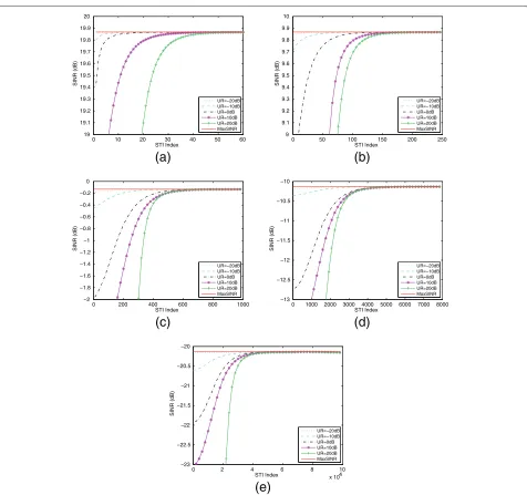
In this section, we provide numerical illustrations of the performances of the proposed Bayesian beamformer. A uniform linear array withN=10 omnidirectional sensors spaced half a wavelength apart is considered. Even though arbitrary noise is applicable to the proposed method, for simplicity, we assume that the noise is a white complex Gaussian with powerσn2=1 in the simulations. A desired source signal is from the broadside and generated as a ran-dom complex Gaussian process with powerσs2. There are
0 10 20 30 40 50 60
19 19.1 19.2 19.3 19.4 19.5 19.6 19.7 19.8 19.9 20
STI Index
SINR (dB)
UR=−20dB UR=−10dB UR=0dB UR=10dB UR=20dB MaxSINR
(a)
0 50 100 150 200 250
9 9.1 9.2 9.3 9.4 9.5 9.6 9.7 9.8 9.9 10
STI Index
SINR (dB)
UR=−20dB UR=−10dB UR=0dB UR=10dB UR=20dB MaxSINR
(b)
0 200 400 600 800 1000
−2 −1.8 −1.6 −1.4 −1.2 −1 −0.8 −0.6 −0.4 −0.2 0
STI Index
SINR (dB)
UR=−20dB UR=−10dB UR=0dB UR=10dB UR=20dB MaxSINR
(c)
0 1000 2000 3000 4000 5000 6000 7000 8000 −13
−12.5 −12 −11.5 −11 −10.5 −10
STI Index
SINR (dB)
UR=−20dB UR=−10dB UR=0dB UR=10dB UR=20dB MaxSINR
(d)
0 2 4 6 8 10
x 104 −23
−22.5 −22 −21.5 −21 −20.5 −20
STI Index
SINR (dB)
UR=−20dB UR=−10dB UR=0dB UR=10dB UR=20dB MaxSINR
(e)
two interferers with the interference-to-noise ratio (INR) 10 dB and 30° and 60° away from the desired signal. Sim-ilar to [27], we define the uncertainty ratio (UR) and the signal-to-noise ratio (SNR), respectively, as
UR=10 log10
where tr{·}denotes the matrix trace. For algorithm ini-tialization, we set C0 = 0.001I, anda0 is drawn from a
complex Gaussian distribution with meanar and
covari-ance matrixC0. The performance evaluation criterion is
the output signal-to-interference-plus-noise ratio (SINR)
SINR(w)=10 log10
In all experiments, the STI block length is set to be K = 512, and the optimum Max-SINR beamformer with the true steering vectoraris provided as reference whose
weight is wMaxSINR = R−i+1nar. In the first experiment,
we investigate the convergence of the proposed method.
−30 −25 −20 −15 −10 −5 0 5 10
−80 −60 −40 −20 0 20 40 60 80 −100
−90 −80 −70 −60 −50 −40 −30 −20 −10 0
Direction (Degree)
Beampattern (dB)
LCMV Subspace Method of [28] Method of [25] Method of [26] Proposed method MaxSINR
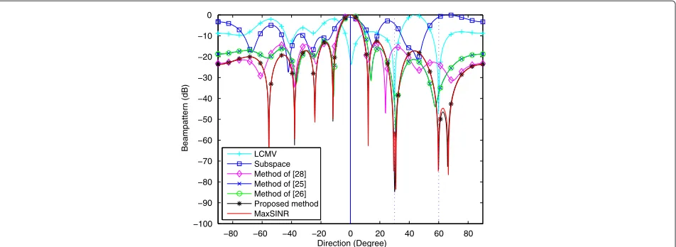
Figure 3Beampatterns of different beamformers from one trial.SNR=10 dB, INR=10 dB, UR= −10 dB, and the results are obtained after 100 STI frames.
Figure 1 shows the output SINR versus STI index for dif-ferent URs under difdif-ferent SNRs. It can be seen that the proposed recursive Bayesian beamformer has good con-vergence performance. With the increase of time, the out-put SINR converges to that of the Max-SINR beamformer for different URs and SNRs. In the case of high SNR and small UR, the convergence is very fast; otherwise, the proposed Bayesian beamformer has slow convergence speed.
For comparison purposes, we also display the perfor-mances of the linearly constrained minimum variance (LCMV) beamformer [29], subspace projection beam-former [22], and other three Bayesian beambeam-formers pro-posed in [25,26,28], where the beamformers of [22,28,29] are non-recursive STI block-based methods and the
beamformers of [25,26] are recursive. For the LCMV
beamformer, the weight iswLCMV = Rˆ
−1
x,ja0
aH
0Rˆ−x,j1a0, where we constrain the weight to satisfy aH0wLCMV = 1 and do not use the diagonal loading. For the subspace projection beamformer, the time-varying (on the STI scale) weight vector is computed asPˆja0, where Pˆj = I− Ud,jUHd,j is
the perpendicular projection matrix for the interference subspace, andUd,jcontains normalized eigenvectors
cor-responding to the two largest eigenvalues in the decom-position Rˆx,j = UjUHj such that Uj =[Ud,j|Us+n,j].
The Bayesian beamforming weight of [27] is σs2(Rˆx,j +
Kσs2C0)−1a0. For the Bayesian methods in [25,26], they
cannot address the uncertainties due to some system-atic problems such as array calibration error and drift
0 100 200 300 400 500 1
2 3 4 5 6 7 8 9 10
STI Index
SINR (dB)
True sigal power Estimated signal power MaxSINR
(a)
0 100 200 300 400 500 0
10 20 30 40 50 60 70
STI Index
Vectorial angle error (Degree)
True sigal power Estimated signal power
(b)
0 100 200 300 400 500 4
5 6 7 8 9 10
STI Index
SINR (dB)
True INCM Estimated INCM (L=1×K) Estimated INCM (L=10×K) Estimated INCM (L=100×K) MaxSINR
(a)
0 100 200 300 400 500
0 10 20 30 40 50 60
STI Index
Vectorial angle error (Degree)
True INCM Estimated INCM (L=1×K) Estimated INCM (L=10×K) Estimated INCM (L=100×K)
(b)
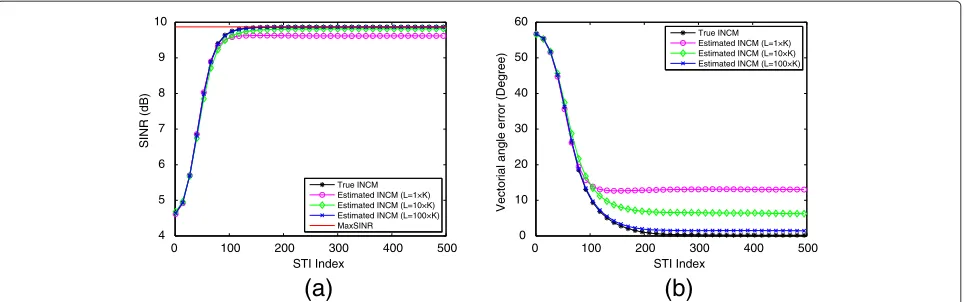
Figure 5The performance of the proposed beamformer with the estimated interference-plus-noise covariance matrix.L=1×K, 10×K, and 100×Ksamples were collected in the absence of the signal of interest, whereK=512, SNR=0 dB, UR=20 dB, and the signal power is known exactly. (a) The output SINR versus STI index for the Max-SINR beamformer and the proposed beamformers with the true and estimated INCM. (b) The vectorial angle error versus STI index for the proposed beamformers with the true and estimated INCM.
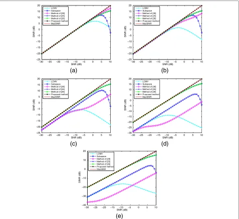
in sensor gains or phases, so the DOA uncertainty is considered here. The source DOA is modeled as a ran-dom variable with prior statistics, and the a prioriPDF of DOA is fixedly set to be uniform at 81 evenly spaced points over [−10◦ : 10◦] in all simulations. Five hun-dred Monte Carlo trials were run for different SNRs and URs. Figure 2 shows the output SINR versus SNR for different beamformers under different URs, where the results are obtained after 80,000 STI frames. The beam-patterns of different beamformers from one trial is shown in Figure 3, where SNR=10 dB, UR= −10 dB, and the STI index is 100. The DOAs of the desired signal and interferers are indicated by the vertical solid and dashed lines, respectively.
From Figures 2 and 3, we can observe that the pro-posed recursive Bayesian beamformer outperforms the other methods and has similar performance to the optimal Max-SINR beamformer. Compared to the LCMV, sub-space projection, and Bayesian method of [28], the pro-posed method produces higher output SINR and better beampattern shape. This is because the proposed beam-former can exploit information about the steering vector contained in past STI windows, while the LCMV, sub-space projection, and method of [28] only simply use the information in the current STI window. Compared to the recursive Bayesian beamformers of [25,26], our method shows some improvements in terms of output SINR and beampattern shape, especially in the case of high SNR. The reason is that we use (25) to calculate the beam-former weights whereRi+nis assumed to be known, while
this assumption is not necessary for the beamformers of [25,26]. In addition, from Figure 2, we can see that the differences between our proposed beamformer and the beamformers of [25,26] are not really significant until some higher SNRs are encountered. The reason is that
there is less information about the steering vector of inter-est contained in the received data when the SNR is much lower. These three Bayesian beamformers have similar performance after convergence, and the SINR improve-ment of our method is insignificant in the case of lower SNRs.
Finally, we assess the performance of the proposed beamformer when the signal power and the interference-plus-noise covariance matrix are inaccurate. As stated in Section 4, we use (26) to estimateσs2and collect a long-term sample covariance estimate forRi+nconsidering the
output of the array in the absence of the signal of inter-est. Besides the output SINR, the vectorial angle error betweenwMMSEj andwMaxSINR is introduced to evaluate the accuracy of beamforming weight, which is defined by
ϑ=arccos
abs{(wMaxSINR)HwMMSEj }
wMaxSINRwMMSE
j
, (30)
where abs{·} denotes the absolute value of a complex number. When this value is close to 0, the proposed beamforming weight in (25) approaches to the Max-SINR beamformer weight.
Figure 4 is shown to assess the performance of the proposed beamformer when the signal power is estimated according to (26), where the interference-plus-noise covariance matrix is known exactly and SNR=0 dB, UR=20 dB. Figure 4a is the output SINR versus STI index for the Max-SINR beamformer, the pro-posed beamformer with true signal power, and estimated signal power. Figure 4b compares the vectorial angle error betweenwMMSEj andwMaxSINRwhen the signal power is known and estimated by using (26).
0 100 200 300 400 500 −5
0 5 10
STI Index
SINR (dB)
True signal power and INCM Estimated signal power and INCM (L=100×K) MaxSINR
(a)
0 100 200 300 400 500
0 10 20 30 40 50 60 70 80
STI Index
Vectorial angle error (Degree)
True signal power and INCM Estimated signal power and INCM (L=100×K)
(b)
Figure 6The performance of the proposed beamformer with the estimated signal power and INCM.(26) is used to estimate signal power, andL=100×Ksamples without signal of interest are collected to estimate INCM, whereK=512, SNR=0 dB, and UR=20 dB. (a) The output SINR versus STI index for the Max-SINR beamformer and the proposed beamformers with the true and estimated signal power and INCM. (b) The vectorial angle error versus STI index for the proposed beamformers with the true and estimated signal power and INCM.
the interference-plus-noise covariance matrix is inac-curate, where the signal power is known exactly and SNR=0 dB, UR=20 dB. In simulations, some long-term samples of the array in the absence of the sig-nal of interest are collected offline to estimate the interference-plus-noise covariance matrix. Here, the length of samples are L = 1 × K, 10 × K, and 100 × K, respectively, where K = 512 is the length of STI. Figure 5a is the output SINR versus STI index for the Max-SINR beamformer and the pro-posed beamformer with true INCM and different esti-mated INCMs, where the INCM is the abbreviation of ‘interference-plus-noise covariance matrix’. Figure 5b shows the vectorial angle error between wMMSEj and wMaxSINR.
From Figures 4 and 5, it can be seen that the proposed Bayesian beamformer with estimated signal power using (26) has similar performance to the beamformer with the true signal power. For the effect of the interference-plus-noise covariance matrix, when the sample length is not long enough, the estimation of Ri+n is inaccurate,
which will result in the inaccuracy of wMMSEj and per-formance degradation of the proposed algorithm. With the increase of sample length, the estimation ofRi+n is
more accurate, and the proposed beamformer has better SINR evaluation and smaller vectorial angle error. Com-pared to the inaccuracy of interference-plus-noise covari-ance matrix, the signal power estimation error affects the performance of the proposed beamformer more slightly, which means that (26) can be used to estimate the sig-nal power in practice. In other words, the accuracy of Ri+n is predominant in the evaluation of the proposed
beamformer. Figure 6 shows the overall performance of the proposed beamformer when signal power is estimated using (26) and 100 × K samples without the signal of
interest are adopted to estimate Ri+n. From Figure 6,
we can see that there is a small performance degrada-tion compared to the proposed beamformer with the true signal power and interference-plus-noise covariance matrix.
6 Conclusions
In this paper, a recursive Bayesian approach is pro-posed to mitigate uncertainty in the steering vector for narrowband beamforming. By assuming that the steering vector is a complex Gaussian random vec-tor, the beamformer can be viewed as a mixture of conditional MMSE estimates weighted by the poste-rior PDF of the random steering vector. To make use of the information about a steering vector contained in past STI windows, a recursive algorithm is devel-oped to estimate the posterior PDF of the steering vec-tor. Simulation results show better performance of the proposed beamformer compared with the LCMV, sub-space projection, and other three Bayesian beamform-ers. After convergence, it has similar performance to the optimal Max-SINR beamformer with true steering vector. A future direction of research consists of gen-eralizing this algorithm to consider the unknown signal power and unknown interference-plus-noise covariance matrix.
Abbreviations
DOA: direction-of-arrival; INCM: interference-plus-noise covariance matrix; INR: interference-to-noise ratio; LCMV: linearly constrained minimum variance; MMSE: minimum mean square error; PDF: probability density function; SINR: signal-to-interference-plus-noise ratio; SNR: signal-to-noise ratio; STI: short-term integration; UR: uncertainty ratio.
Competing interests
Acknowledgments
This study is supported in part by the National Natural Science Foundation of China (grant no. 11273017). The authors would like to thank Dr. Karl F. Warnick and Dr. Brian D. Jeffs, Department of Electrical and Computer Engineering, Brigham Young University, for their valuable comments and suggestions which greatly improved the paper.
Author details
1School of Electronic and Optical Engineering, Nanjing University of Science &
Technology, Nanjing, 210094, China.2College of Engineering, Nanjing
Agricultural University, Nanjing, 210031, China.
Received: 15 September 2012 Accepted: 4 May 2013 Published: 21 May 2013
References
1. BD Van Veen, KM Buckley, Beamforming: a versatile approach to spatial filtering. IEEE Acoust, Speech, Signal Process. Mag.5(2), 4–24 (1988). doi:10.1109/53.665
2. HL Van Trees,Optimum Array Processing. (Wiley Interscience, New York, 2002)
3. BD Jeffs, KF Warnick, J Landon, J Waldron, D Jones, JR Fisher, ND Norrod, Signal processing for phased array feeds in radio astronomical telescopes. IEEE J. Sel. Top. Sig. Proc.2(5), 635–646 (2008).
doi:10.1109/JSTSP.2008.2005023
4. E Habets, J Benesty, I Cohen, S Gannot, J Dmochowski, New insights into the MVDR beamformer in room acoustics. IEEE Trans. Audio Speech Lang. Process.18(1), 158–170 (2010). doi:10.1109/TASL.2009.202
5. EA Gharavol, Y-C Liang, K Mouthaan, Robust downlink beamforming in multiuser MISO cognitive radio networks with imperfect channel-state information. IEEE Trans. Vehicular Technol.59(6), 2852–2860 (2010). doi:10.1109/TVT.2010.2049868
6. O Besson, F Vincent, Performance analysis of beamformers using generalized loading of the covariance matrix in the presence of random steering vector errors. IEEE Trans. Signal Process.53(2), 452–459 (2005). doi:10.1109/TSP.2004.840777
7. T-T Lin, F-H Hwang, inProc. International Conference on Network and Electronics Engineering, vol. 11. A robust beamformer against large pointing error (IACSIT Press, Singapore, 2011), pp. 9–13
8. C Zhang, J-Q Ni, Y-T Han, G-K Du, in5th International ICST Conference on Communications and Networking in China. Performance analysis of antenna array calibration and its impact on beamforming: a survey (IEEE, New York, 2010), pp. 1–5
9. Z Yermeche, N Grbic, I Claesson, inProc. IEEE Workshop on Applications of Signal Processing to Audio and Acoustics. Beamforming for moving source speech enhancement (IEEE, New York, 2005), pp. 25–28
10. M Wax, Y Anu, Performance analysis of the minimum variance beamformer. IEEE Trans. Signal Process.44(4), 928–937 (1996). doi:10.1109/78.492545
11. RG Lorenz, SP Boyd, Robust minimum variance beamforming. IEEE Trans. Signal Process.53(5), 1684–1696 (2005). doi:10.1109/TSP.2005.845436 12. J Li, P Stoica, Z Wang, On robust Capon beamforming and diagonal
loading. IEEE Trans. Signal Process.51(7), 1702–1715 (2003). doi:10.1109/TSP.2003.812831
13. LC Godara, MRS Jahromi, Convolution constraints for broadband antenna arrays. IEEE Trans. Antennas Propagation.55(11), 3146–3154 (2007). doi:10.1109/TAP.2007.908823
14. S-T Zhang, ILJ Thng, Robust presteering derivative constraints for broadband antenna arrays. IEEE Trans. Signal Process.50(1), 1–10 (2002). doi:10.1109/78.972477
15. CY Chen, PP Vaidyanathan, Quadratically constrained beamforming robust against direction-of-arrival mismatch. IEEE Trans. Signal Process.
55(8), 4139–4150 (2007). doi:10.1109/TSP.2007.894402
16. N Grbic, S Nordholm, inIEEE International Conference on Acoustics, Speech, and Signal Processing, vol. 1. Soft constrained subband beamforming for hands-free speech enhancement (IEEE, New York, 2002), pp. 885–888 17. SA Vorobyov, AB Gershman, Z-Q Luo, Robust adaptive beamforming
using worst-case performance optimization: a solution to the signal mismatch problem. IEEE Trans. Signal Process.51(2), 313–324 (2003). doi:10.1109/TSP.2002.806865
18. H-H Chen, AB Gershman, inIEEE International Conference on Acoustics, Speech and Signal Processing. Worst-case based robust adaptive beamforming for general-rank signal models using positive semi-definite covariance constraint (IEEE, New York, 2011), pp. 2628–2631
19. J Foutz, A Spanias, S Bellofiore, CA Balanis, inIEEE Antennas Wireless Propagation Lett, vol. 2. Adaptive eigen-projection beamforming algorithms for 1D and 2D antenna arrays, (2003), pp. 62–65. doi:10.1109/LAWP.2003.811322
20. A Pezeshki, BD Van Veen, LL Scharf, H Cox, ML Nordenvaad, Eigenvalue beamforming using a multirank MVDR beamformer and subspace selection. IEEE Trans. Signal Process.56(5), 1954–1967 (2008). doi:10.1109/TSP.2007.912248
21. J Raza, AJ Boonstra, Veen van der A J, Spatial filtering of RF interference in radio astronomy. IEEE Signal Process. Lett.9(2), 64–67 (2002).
doi:10.1109/97.991140
22. BD Jeffs, KF Warnick, Spectral bias in adaptive beamforming with narrowband interference. IEEE Trans. Signal Process.57(4), 1373–1382 (2009). doi:10.1109/TSP.2008.2011841
23. S Sirianunpiboon, SD Howard, J Asenstorfer, inProc. IEEE Workshop on Sensor Array and Multichannel Processing. A hierarchical Bayesian approach to direction finding and beamforming (IEEE, New York, 2006), pp. 21–25 24. Y Bucris, I Cohen, MA Doron, Bayesian focusing for coherent wideband
beamforming. IEEE Trans. Audio Speech Lang. Process.20(4), 1282–1296 (2012). doi:10.1109/TASL.2011.2175384
25. KL Bell, Y Ephraim, HL Van Trees, A Bayesian approach to robust adaptive beamforming. IEEE Trans. Signal Process.48(2), 386–398 (2000). doi:10.1109/78.823966
26. CJ Lam, AC Singer, Bayesian beamforming for DOA uncertainty: theory and implementation. IEEE Trans. Signal Process.54(11), 4435–4445 (2006). doi:10.1109/TSP.2006.880257
27. O Besson, AA Monakov, C Chalus, Signal waveform estimation in the presence of uncertainties about the steering vector. IEEE Trans. Signal Process.52(9), 2432–2440 (2004). doi:10.1109/TSP.2004.831917 28. CJ Lam, AC Singer, inProc. Int. Conf. Acoustic, Speech, Signal processing,
vol. 4. Adaptive Bayesian beamforming for steering vector uncertainties with order recursive implementation (IEEE, New York, 2006), pp. 997–1000 29. CY Tseng, LJ Griffiths, A unified approach to the design of linear
constraints in minimum variance adaptive beamformers. IEEE Trans. Antennas Propagat.12, 1533–1542 (1992). doi:10.1109/8.204744
doi:10.1186/1687-6180-2013-108
Cite this article as:Han and Zhang:A recursive Bayesian beamforming for
steering vector uncertainties.EURASIP Journal on Advances in Signal Process-ing20132013:108.
Submit your manuscript to a
journal and benefi t from:
7Convenient online submission 7Rigorous peer review
7Immediate publication on acceptance 7Open access: articles freely available online 7High visibility within the fi eld
7Retaining the copyright to your article