Simple Models for Diffusion in Thin Plates or Membranes

(1)

http://www.scirp.org/journal/jamp ISSN Online: 2327-4379

ISSN Print: 2327-4352

DOI: 10.4236/jamp.2019.77105 Jul. 24, 2019 1547 Journal of Applied Mathematics and Physics

Simple Models for Diffusion in Thin Plates

or Membranes

Jorge Corrêa de Araújo , Rosa García Márquez

State University of Rio de Janeiro, DMAT-FFP, Rio de Janeiro, Brazil

Abstract

Two simplified models, linear and nonlinear, were used in a cementation process on a homogeneous thin carbon steel plate. The parameters for these models, as obtained by the least squares’ method the first one in a global way while the other parameters refer to the second model—were estimated by a set of local minimums. To compare the performance of these models we used theoretical data, for the same diffusion problem obtained by a one-dimensional transient model considering the concentrations in the mean plane of the plate. The results for carbon concentrations in weight percentage in the plate (%pC) as a time-only dependent function with these simplified models to represent the analyzed diffusion process were in good agreement with those from a stricter model. The diffusion flows of these models were determined and a reasonable agreement can be seen in relation to the flow obtained by the theoretical model on the surface of the plate. This study shows that it is possible to use this methodology with the given restrictions adopted here to describe the concentration and the diffusion flow of other solutes in thin membranes.

Keywords

Simplified Model, Theoretical Model, Membrane, Mean Concentration

1. Introduction

The one-dimensional diffusion in a medium is limited by two parallel planes, for example, in x=0 and x=L_{of such thin thickness, so that the entire} diffu-sive process occurs through these sheets or membranes, while only a negligible amount occurs through the lateral faces, which is well known [1] [2]. In particu-lar, if on the face x=0 the concentration of the diffusing substance is constant

and equal to C1 and on the other x=L it is a constant C2, and if the initial

How to cite this paper: de Araújo, J.C. and Márquez, R.G. (2019) Simple Models for Diffusion in Thin Plates or Membranes. Journal of Applied Mathematics and Phys-ics, 7, 1547-1559.

https://doi.org/10.4236/jamp.2019.77105

Received: June 26, 2019 Accepted: July 21, 2019 Published: July 24, 2019

http://creativecommons.org/licenses/by/4.0/

(2)

DOI: 10.4236/jamp.2019.77105 1548 Journal of Applied Mathematics and Physics concentration is uniform and equal to a constant C0, the concentration C x t

( )

,

can be obtained from the transient diffusion equation in a one-dimensional medium with a constant diffusion coefficient D given by 22

C C

D

t x

∂ ∂

= ∂

∂ [2] using, for

example, the method of separating variables or through the Laplace Transform

[3]. The solution of this problem via the separation of variables involves an infi-nite series of sine terms combined with an exponential function with a negative factor in each term of the series, which albeit complicated, quickly converges, except for small values of [4]. The solution obtained by the Laplace Transform lies in the calculation of the erf x

( )

function or Gauss error function, whose values are given in tables for different values of

2

x

Dt . In general, diffusion is three-dimensional process, but sometimes the problem is simplified using a smaller number of dimensions. According to Fox et al. [5], for many problems found in engineering, a one-dimensional analysis is adequate to provide ap-proximate solutions with the precision required in engineering practice. Recent-ly, Araújo e Márquez [6] used transient one-dimensional diffusion in a cement-ing process of a homogeneous metal sample of carbon steel with a thickness of less than two millimeters to obtain information on carbon concentration in a semi-infinite plate where the Gauss error function was replaced by a fifth-degree polynomial.

The cementation process consists of the hardening of the surface of steel to higher levels to that of its interior by the diffusion or transport of carbon atoms at high temperatures in an atmosphere rich in hydrocarbon gas such as CH4 methane gas [7]. The question we pose in this article is whether there is a simp-ler model that can be adopted to estimate the concentration of carbon in diffu-sion in thin plates or membranes. Although recognizing that the process of dif-fusion of materials through cell membranes is quite complicated, Bassanezi and Ferreira Jr. [8] and Bassanezi [9] presented two diffusion models through cell membranes based on a simplification of Fick’s Law [7]. These diffusion models are applied when the concentration difference between the cell medium and the homogeneous liquid medium where the cell is immersed is small and the cell has the area and volume constant throughout the process. For this, it is also assumed in a natural way that the flow of molecules goes in both directions until the con-centration inside the cell is equal to the concon-centration of the medium it is sus-pended in. The first model is represented by the linear ordinary differential equ-ation given by

( )

d

d e

C kA

C C t

(3)

DOI: 10.4236/jamp.2019.77105 1549 Journal of Applied Mathematics and Physics structure of the membrane, so it needs to be estimated for each situation. The second model, also simplified, but with two parameters, is given by an ordinary non-linear differential equation as

( )

(

)

(

( )

)

2

1 2

d

e

e e

C t C _A

k C C t k C C t

t V

−

 

 ₌ _ ₋ ₊ ₋ _

 

 . (2)

The term in square brackets is the function for solute flowing into the cell [8]. According to Bassanezi and Ferreira Jr. [8], the experimental obtaining of the constant can be difficult and sometimes impossible to obtain, in which case the two-parameter model can be useful for the theoretical analysis of the problem understudy, but not for the specific study. Although agreeing that the experi-mental achievement of these parameters is not trivial, their estimates are possible in our understanding, provided that experimental data

(

t C t_i,

( )

_i

)

can be ob-tained by some experimental or theoretical means. In this sense, the purpose of this paper is to solve in detail the differential equation of the model with two pa-rameters and, from the theoretical data estimated by a transient one-dimensional diffusion model of carbon diffusion in a thin homogeneous sample of carbon steel of thickness to one millimeter, to estimate the k1 parameter of the linear

model using the linear least squares’ or linear regression method and the k1

and k2 parameters of the non-linear model, using the non-linear least squares’

method. These parameters are related to the medium where the diffusion occurs. The results show that there was good agreement among the models adopted in this study with the results of the carbon concentrations estimated by the one-dimensional model of transient diffusion on the plane of the plate x=0.0005 m or mem-brane. Thus, the simplified models, in particular the one-parameter model, gave a good description of the problem analyzed, providing a semi-qualitative mean value for the concentration within the plate at any point and instant in the x di-rection.

2. Materials and Methods

Consider a homogeneous metal plate formed by an Iron-gamma Carbon alloy, in-dicated by, Feγ-C which hast to be hardened through a process of cementation [7]. The steel part is exposed in an atmosphere rich in hydrocarbon gas (such as methane gas, CH4), under T =1000 C . The homogeneous plate with the properties shown

in Table 1, has an uniform concentration of carbon C0=C x

( )

, 0 =0.08% pC

(weight percent carbon) for 0< <x L. The carbon concentration is kept con-stant and equal C1=C

( )

0,t =0.10% pC to the flat face x=0, and also

con-stant and equal C2 =C L t

( )

, =0.10% pC to the flat face x= =L 0.001 m with 0

t≥ . Under these conditions, the goal is to obtain theoretical data on the process at different moments in time, in hours for the mean plane of the plate, that is, in x=0.0005 m. Figure 1 shows in simplified form the metal plate sub-jected to the conditions given in the cementation process described above.

(4)

[image:4.595.282.467.66.174.2]

DOI: 10.4236/jamp.2019.77105 1550 Journal of Applied Mathematics and Physics

[image:4.595.209.536.223.447.2]

Figure 1. Carbon transient diffusion moving through a thin carbon steel plate.

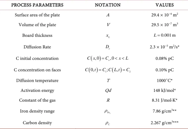
Table 1. Parameters considered in the cementation process.

PROCESS PARAMETERS NOTATION VALUES

Surface area of the plate A 29.4 × 10−4_m2

Volume of the plate V 29.5 × 10−7_m3

Board thickness xL L=0.001 m

Diffusion Rate Do 2.3 × 10

−5_m2_/s*

C initial concentration C x( ), 0 =Co, 0< <x L 0.08% pC

C concentration on faces C

( )

0,t =C C L t1;

( )

, =C2 0.10% pC

Diffusion temperature T 1000˚C*

Activation energy Qd 148 kJ/mol*

Constant of the gas R 8.31 J/mol∙K*

Iron density range ρFeγ 7.86 g/cm

3_**

Carbon density ρC 2.267 g/cm3***

*Reference value obtained for this diffusion (Callister, 2002, p. 70, Table 5.2). **Reference value obtained for this diffusion (Callister, 2002, p. 537, Table B.1). ***https://iupac.org/. Union of Pure and Applied Chemistry (IUPAC)

occurs through the lateral faces [1] [2].

Table 1 shows the parameters for the carburizing process, notation and

as-sumed values, and the initial conditions of the diffusion process.

2.1. Linear Least Squares: Discrete Case

Given a set of points

(

x y_i, _i= f x

( )

_i

)

, i=1,,n and a≤x_i≤b, the goal is to choose g xi

( )

continuous real functions in the I=

[ ]

a b, interval to obtain

constants or parameters λ1,,λn so that

( )

1

n

i i i

x g x f x

φ λ

=

∑

≅ _{. (3)}

As the λi coefficients appear linearly in the definition of the

ϕ

( )

x

ap-proximation function, this model is called linear [10]. The choice of

ϕ

( )

x model depends on the

(

x yi, i = f x

( )

i

)

dispersion diagram, or in other words

of the tabulated points. Be Rk = f x

( ) ( )

k −

φ

xk the k-th residue of this

(5)

( )

(

)

2

1 1 , , m n i i

F λ F λ λ R

=

=  =

∑

(4)

where mn. To get a F

( )

λ

minimum point of it is necessary to solve the equation of the critical points given by

( )

0

F

λ

∇ =. (5)

The equations obtained from Equation (5) give rise to a linear system of

n n

×

order given by

Aλ=b,

(6) where, according to Ruggiero e Lopes [10] matrix entries can be obtained by

,

ij i j

a = g g ; bi = y g, i ,

(

( )

)

T

1 , ,

i i i m

g = g x  g x being

( )

(

)

T

1 , , m

y= f x  f x , with i j, =1,,n and , denotes the scalar product in m

IR space. If the matrix is invertible, it is obtained

λ

=

(

λ

1,,

λ

n

)

in an

unique way of Equation (6).

2.2. Nonlinear Least Squares: Discrete Case

If

φ

( )

x it is not a linear model of the parameters as in Equation (3), the equa-tion of the critical points no longer produces a linear system as obtained in Equ-ation (6). Consider

( )

(

( )

)

T 1

:

, , .

n m

m

R U IR IR

R λ R λ R λ

⊂ →

= _

(7)

Therefore, as R

( )

λ

is a vector function for residues in the Rm space and

( )

(

,

)

i xi

ϕ λ

=

ϕ

λ

_{is the nonlinear model for adjustment point}

(

x y_i, _i = f x

( )

_i

)

,

1, ,

i=  m and a≤x_i≤b, where λ=

(

λ₁,,λ_n

)

T is a vector of adjustable

parameters of the n

IR space. With this notation, the k-th residue of this ap-proximation is defined by Rk

( )

λ

= f x

( ) (

k −

φ

xk,

λ

)

, k=1,,m. The objec-tive is to minimize F

( )

λ as in Equation (4), that is, the Equation (5) of the critical points is written thus

( ) (

)

1

,

0, 1, ,

m

i i

i k

x

R λ φ λ k n

λ =

∂

= =

∂

∑



(8)

Using a Taylor series expansion [11] to the first order for each Ri

( )

λ

coor-dinate function around λ, being

(

)

T

1, , n

p= p  p an increment vector we have

(

)

( )

i i i

R

λ

+p =R

λ

+ ∇R

λ

p, (9)

where

( )

1 , , i i i n R R

R λ λ λ

λ λ

∂ ∂

 

∇ =  _∂ _∂ 

  , with i=1,,m. From Equations ((8), (9)) it is k=1,,n

( )

(

)

(

)

1 1 , , 0 n

m i i

i j

i

j j k

x x

R λ φ λ p φ λ

λ λ = =  ∂ ∂ + =  _∂  _∂    

∑

. (10)

(6)

DOI: 10.4236/jamp.2019.77105 1552 Journal of Applied Mathematics and Physics given by

( )

(

)

(

)

(

)

(

)

1 1 1 1 , , , , n m m n x x J x x

φ λ φ λ

λ λ

λ

φ λ φ λ

λ λ ∂ ∂    _∂ _∂      =   ∂ ∂    _∂ _∂        

. (11)

From Equations ((10), (11)) we have a linear system of

n n

×

order given by

( ) ( )

T T

J

λ

J

λ

p= −J

λ

R

λ

. (12)

Equation (12) is the basis for an iterative process and is known as a modified Newton method [12]. Taking

(

)

T

0 0 0

1, , n

p = p  p as an initial approximation, we calculate J

( )

λ

, T

( )

J

λ

and R

( )

λ

using p0. Then the system given by Equation (10) is solved to obtain the p value. The vector 1 0

p = p +p is eva-luated, for example, by the sum of the quadratic residuals, that is, if

( )

₁ 2

( )

₁ 2

1

m

i i

R p R p tol

=

∑

< _then, 1

p it is a solution by least squares, where tol is the tolerance allowed in the approximation. If 1

p it is not the best solution for the least squares, new iterations are performed until convergence can be achieved.

2.3. The One-Dimensional Diffusion Equation

The solution of the transient one-dimensional diffusion equation for the diffu-sion problem in thin membranes with constant surface concentrations and ini-tial distribution with uniform concentration, that is,

( )

1 0,

C =C t , C2 =C L t

( )

, ;t≥0 and C0=C x

( )

, 0 ; 0< <x L,

(13)

can be obtained by the method of separation of variables, whose solution is given according to Crank [2] by

( )

(

)

( ) 2 2 2 2 2 2 π 2 1 2 1 1 1

2 1 π

0

cos π

2 π

, sin e

π

2 1 π

4 1

sin e

π 2 1

Dn t L n

D m t L m

C n C

C C n x

C C x t C x

L n L

m x C m L − ∞ = − + ∞ = −   −     = = +  +   _ _     +     + _ _ _ _ +    

∑

(14)

3. Results and Discussions

Model 1 as given and reported by Equation (1) is given by

( )

d

d e

C kA

C C t

(7)

( )

0 0

d

C t

e C

C A

k t

C −C t = V

∫

. (16)

From Equation (16) results the C t

( )

expression for given by

( ) (

0

)

e

A k t

V

e e

C=C t = C −C − +C ,

(17)

where C0=C

( )

0 . Note that C t

( )

→Ce when t→ ∞.

In Equation (15), an analogy with Fick’s first law for one-dimensional diffusion in a steady state [7], making it possible to interpret the term J= ⋅k Ce−C t

( )



as the amount of mass that crosses the membrane per unit area, in a given direc-tion per unit of time. Model 2, as proposed by Bassanezi and Ferreira [8] and al-ready mentioned in the introduction (Equation (2)) is given formally by

( )

(

)

(

( )

)

2

1 2

d

e

e e

C t C _A

k C C t k C C t

t V

−

 

 ₌ _ ₋ ₊ ₋ _

 

 . (18)

Making f C

( )

=F C

(

e−C

)

where F C

(

e−C

)

it is denominated by the

au-thors as a function for flow based on the difference of concentrations, where f C

( )

is a real function of a real variable, and wheref C

( )

_e =F C

(

_e−C_e

)

=F

( )

0 =0.

To justify this fact we assume the plausibility where if there is no difference of concentration there should be no flow between the means. Assuming f C

( )

is at least 3

(

)

,

C I R class function; where I=

[ ]

0,t0 [11] using a Taylor series

expansion of up to the second order around has [11],

(

)

( )

(

( )

)

( )

(

( )

)

2

e

e e e e e

f C

f C −h = f C +f′ C C −C t + ′′ C −C t , (19)

or,

( )

(

( )

)

( )

0

(

( )

)

2

0

2

e e

F

f C =F′ C −C t + ′′ C −C t . (20) From Equation (15) we have seen that J = ⋅k Ce−C t

( )

 represents a flow

of molecules into the cell, then replacing that term with the given f C

( )

flow function as in Equation (18), we obtain the two-parameter formulation for cell diffusion only reported by Bassanezi and Ferreira Jr. [8] to obtain Equations (2) or (18),

(

)

(

( )

)

(

( )

)

2

1 2

d

d e e e

A

C C k C C t k C C t

t V

 

− = __ − + − ___{, (21)}

where, k1=kF′

( )

0 and

( )

2

0 2

F

k =k ′′ . For the physical sense of the problem, the unity of k1 is the same as of k, that is, m/s, while the unity k2 of can be

giv-en as, m4_{/kg∙s. Making}

e

y= −C C the Equation (21) rewrite in the form

2

1 2

d d

k A k A

y

y y

t + V = V . (22) Equation (22) is a Bernoulli equation [13] and can be solved by changing the variable as 1

(8)

1 2

d d

k A k A

u u

t − V = − V .

(23) Equation (23) can be solved using the

( )

e 1

k A t V

t

µ = − _{integral factor to obtain}

1

1 2

1

e

k A t V

Kk k

u

k +

= .

(24)

Using the fact that 1

u=y− and y

( )

0 =C₀−C_e follows from Equation (23) the solution to Equation (21) given by

(

)

(

)

1

(

)

1 0

2 0 e 1 2 0

e

e k A

t V

e e

k C C C C

k C C k k C C

− = +

 

− + _ − − _

.

(25)

Note what C

( )

0 =C0 and C t

( )

→Ce when t→ ∞ . In particular, if

( )

0 1

F′ = and F′′

( )

0 =0 and only then, the differential equation describing model 1, as given by Equation (13) is retrieved. However, if F′

( )

0 ≠1 and

( )

0 0

F′′ = , the constant k1=kF′

( )

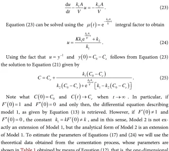
0 ≠k, and in this sense, Model 2 is not

[image:8.595.205.540.70.368.2] [image:8.595.271.475.565.728.2]

ex-actly an extension of Model 1, but the analytical form of Model 2 is an extension of Model 1. To estimate the parameters of Equations (17) and (24) we will use the theoretical data obtained from the cementation process, whose parameters are shown in Table 1 obtained by means of Equation (12), that is, the one-dimensional transient diffusion model (MD) or as we will call theoretical model.

Table 2 shows the estimates in %pC at the x=0.0005 m plane position in

several time using ten terms of the series defined by the Equation (14), so that the values with number of major terms would not provide significant concentra-tions variaconcentra-tions. The choice of the mean plane of the plate or membrane was to assume that the solute concentration at this depth of the plate would represent a mean concentration (inside the plate), and thus, the estimates obtained for the parameters of the simplified models would “mirroring” in a semi-qualitatively way this mean concentration.

The permeability parameter (Model 1) can be obtained through the global minimum with the linearization of Equation (15) according to the procedure

Table 2. Estimates for %pC in the membrane with MD.

Time (hours) %pC (MD)

0.0 0.0008000

0.5 0.0008231

1.5 0.0009089

2.0 0.0009353

3.0 0.0009674

5.0 0.0009917

7.0 0.0009979

(9)

DOI: 10.4236/jamp.2019.77105 1555 Journal of Applied Mathematics and Physics described in Section 2.1. doing y= −C Ce, and therefore Equation (15) is

re-written thus

(

0

)

e

Ak t V e

y C C

− = − .

(26)

In applying the Neperian Logarithm to Equation (26) we obtain

( )

(

0

)

ln ln _e kA

z y C C t

V

= − = − − _.

₍₂₇₎

Thus, using the discrete points in Table 2 we can write

i i

z = +B λt ,

(28)

where z_i =ln

(

C_e−C t

( )

_i

)

, B=ln

(

Ce−C0

)

and

kA V

λ= − . As B is constant,

Equation (28) can be reduced to a linear form given by

i i

w =λt , (29) which wi = −zi B. Therefore Equation (28) can be solved by rewriting Equation

(1) as,

ϕ λ

( )

t, =

λ

t being g t₁

( )

=t. Thus, the matrix of the system given by

Equation (4) is of an order of 1 1× , that is,

7 2 11 1 1

1

, i

i

a g g t

=

= =

∑

_,

7

1 1

1

, _i _i

i

b y g t w

=

= =

∑

_{. Hence, Equation (6) gives the first-order linear equation}

given by

11 1

104.4298

0.612491 170.50

a λ= ⇒ = −b λ = − . (30)

As a result, kA V

λ= − _and_A_,_V_{are given as shown in}_{Table 1}_,

4

6.12491 10

k= × − , with

(

)

(

)

2 2

0 0 9

1

1.0441 10

m

i i

R p k R p k −

=

= =

∑

= = × _{. Now}

Equation (15) is fully determined.

To estimate the Model 2 parameters, we used the non-linear least squares’ method described in Section 2.2. From Equation (24) two models were proposed: the model named MD21, where only the k2 parameter was allowed to vary

while k1 =k and Model MD22, where both parameters varied. The initial

pa-rameter vector for MD21 was 0 21 0.01

p = with a tolerance 4

10

tol= − and con-vergence occurring in only two cycles for the value of 2

2 1.9224

k = , where

( )

₂ 2

( )

₂ 2 ₉

21 21 1 1.0567 10 m i i

R p R p −

=

∑

= × _{. For MD22, the initial parameter vector}

was taken as 0

(

)

T 22 0.0007,1.0

p = with a tolerance tol=10−5 and convergence also occurring in two cycles for the

(

)

T

2 2 2

22 1 0.0004, 2 3.4907

p = k = k = , the vector

being

( )

₂ 2

( )

₂ 2 ₉

22 22 1 1.0544 10 m i i

R p R p −

=

∑

= × _{. Please note that in terms of}

qua-dratic residues, there is no significant difference between these iterative models. The relative percentage error for MD1, εMD1 in relation to the estimates of

(10)

DOI: 10.4236/jamp.2019.77105 1556 Journal of Applied Mathematics and Physics Similarly, for MD21, εMD21<6.2% while for the MD22 model, εMD22<6.5%.

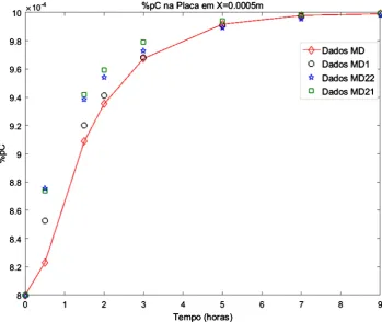
[image:10.595.186.536.396.690.2]

The highest divergence between concentrations took place in the t≤2.0 h time interval. Based on the criteria analyzed, and because the MD1 model has its parameter estimated in a global way, and due to its greater simplicity, it is at first the model to be adopted to estimate the mean carbon concentration in the thin plate. Figure 2 shows the adjustment in the half-plane estimated in %pC ob-tained with the different adjustment models analyzed.

Figure 2 confirms that the best fit was with MD1 followed by MD22 and

fi-nally by MD21 in relation to the theoretical data estimated by the MD model as given by the solid line. The MD22 model when varying the initialization vector

(

)

T

0

22 0.0007,1.0

p = showed instability, probably due to the sensitivity of these parameters and, therefore, the

(

)

T

2 2 2

22 1 0.0004, 2 3.4907

p = k = k = was chosen

from a set of global minimums. This instability also occurred during the refine-ment of the parameter in the MD21 model.

One of the advantages of these simplified models is that their expressions for

( )

C t are analytical, as opposed to the solution obtained by Equation (14) which is given in terms of an infinite series. Figure 2 shows a little more, that is, on the more superficial layers it is expected that models MD21 and MD22 are closer to the estimates of theoretical concentrations, as a greater spread is seen above the continuous graph obtained by the MD model for the mean plate plane.

If we consider the x=0.00025 m plane of the plate, the maximum percentage

Figure 2. Comparison of the MD1, MD21 and MD22 models with the MD model at the 0.0005 m

(11)

DOI: 10.4236/jamp.2019.77105 1557 Journal of Applied Mathematics and Physics difference between the concentrations estimated by the MD1 model for the

0.0005 m

x= plate plane are lower than 2% when compared with the theoretical data (not shown here), for the estimates of the concentrations in x=0.00025 m obtained by the MD model. This allows us to assume that the simplified model to a parameter can estimate, in a semi qualitative way, the %pC concentrations inside the plate or thin membrane, and without the need to use iterative me-thods where the global minimum cannot be obtained. Unlike the MD model, the diffusion of the simplified models lies in the analytical functions. That is, from Equation (15) the diffusion flow function is given by J1= ⋅k Ce−C t

( )

, while in Equation (20), the diffusion flow is given by

(

( )

)

(

( )

)

2

2 1 e 2 e

J =k C −C t +k C −C t . From Equation (12) the diffusion flow across the face is given using [2].

( )

2 2 2 2

2 2

2 1 π π

0

2 1

1 0

0,

4 2

cos π e e

D n Dm

t t

L L

m n

C t

J D

t

C

D C m C

L L

+

∞ − ∞ −

= =

∂ = −

∂

 

 

= − _ _ − _ + _

 



∑



(31)

The flow functions from simple models are dependent on the difference in concentration between the media, so it is to be expected that the J2 flow will

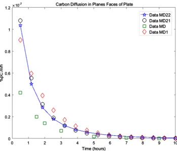
be less pronounced than the J1 flow. Figure 3 clearly shows that the largest

[image:11.595.185.536.396.695.2]

difference in concentration occurs in models MD21 and MD22 in relation to the theoretical concentrations, and thus the Ce−C t

( )

terms are smaller in relation

(12)

DOI: 10.4236/jamp.2019.77105 1558 Journal of Applied Mathematics and Physics to the same terms of the MD1 model, indicating that the diffusion for models MD21 and MD22 is “less apparent” in relation to the J1 model. Figure 3

shows the carbon diffusion profile diffusion on the flat faces of the plate, con-firming this observation.

After two hours of the cementation process, the carbon transfer rates through the flat section on the surface of the plate were in good agreement when com-pared with the data provided by the theoretical model. A possible explanation for the discrepancy of flows estimated by the simplified models for times under two hours can be credited to the fact that the parameters estimated for the mod-els were based on the data of the theoretical concentrations obtained for the mean plane, and not the surface plane where the concentration was kept fixed during the cementation process.

4. Conclusion

The analyzes showed that the simplified diffusion models in cell membranes analyzed in this study may be an alternative to the transient one-dimensional models used for the description of membrane diffusion processes. The simplest models depend on parameters that can be obtained globally using known func-tion adjustment methods, such as that of the least squares. In particular, they were used to obtain percentages by weight of carbon in a cementation process with restricted thickness conditions. The results obtained were in good agree-ment when compared with the estimates of the theoretical model used for this purpose. The simplified model with one parameter was shown to be the best op-tion to represent the average estimate of the concentraop-tion of carbon solute in the diffusion process due to the concentration difference on the plate or mem-brane, and this is due to the fact that this model uses only one parameter and that it can be obtained non-iteratively; that is, in a global way.

Conflicts of Interest

The authors declare no conflicts of interest regarding the publication of this pa-per.

References

[1] Carslaw, H.S. and Jaeger, J.C. (2011) Conduction of Heat in Solids. 2nd Edition, Clarendon Press, Oxford.

[2] Crank, J. (2011) The Mathematics of Diffusion. 2nd Edition, Clarendon Press, Ox-ford.

[3] Churchill (1972) Operational Mathematics. 3rd Edition, McGraw-Hill, New York. [4] Boyce, W.E. and Diprima, R.C. (1999) Equações Diferenciais Elementares e

Problemas de Valores de Contorno. 6th Edition, LTC, Rio de Janeiro.

[5] Fox, R., Pritchard, P.J. and McDonald, A.T. (2011) Introdução à mecânica dos fluidos. 7th Edition, Tradução e revisão técnica de Ricardo Koury e Luiz Machado. Editora LTC, Rio de Janeiro.

(13)

DOI: 10.4236/jamp.2019.77105 1559 Journal of Applied Mathematics and Physics concentração de carbono em amostras metálicas de aço-carbono. Revista Eletrônica da Matemática, 4, 215-228.

[7] Callister, W.D. (2002) Ciência e Engenharia de Materiais: Uma Introdução. 5th Edition, LTC, Rio de Janeiro, Brazil.

[8] Bassanezi, R.C. and Ferreira, W.C. (1988) Equações Diferenciais com Aplicações. ed. Harbra, São Paulo, Brazil.

[9] Bassanezi, R.C. (2002) Ensino Aprendizagem com Modelagem Matemática. 3rd Edition, ed. Contexto, São Paulo, Brazil.

[10] Ruggiero, M.A.G. and Lopes, V.L.R. (2006) Cálculo Numérico Aspectos Teóricos e Computacionais. 2nd Edition, Pearson Makron Books, São Paulo, Brazil.

[11] Lima, E.L. (2016) Curso de Analise. Vol. 1, ed. IMPA, Rio de Janeiro, Brazil, 14. [12] Neto, A.J.S. and Neto, F.D.M. (2005) Problemas Inversos. Conceitos Fundamentais

e Aplicações. Ed. UERJ, Rio de Janeiro, Brazil.