A Bayesian Inference of Non-Life Insurance Based on
Claim Counting Process with Periodic Claim Intensity
Uraiwan Jaroengeratikun, Winai Bodhisuwan, Ampai Thongteeraparp
Department of Statistics, Kasetsart University, Bangkok, Thailand Email: [email protected], {fsciwnb, fsciamu}@ku.ac.th
Received January 22, 2012; revised February 25, 2012; accepted March 10, 2012
ABSTRACT
The aim of this study is to propose an estimation approach to non-life insurance claim counts related to the insurance claim counting process, including the non-homogeneous Poisson process (NHPP) with a bell-shaped intensity and a beta-shaped intensity. The estimating function, such as the zero mean martingale (ZMM), is used as a procedure for parameter estimation of the insurance claim counting process, and the parameters of model claim intensity are estimated by the Bayesian method. Then,
t , the compensator of N t
is proposed for the number of claims in a time in-terval
0,t
. Given the process over the time interval
0,t
, the situations are presented through a simulation study andsome examples of these situations are also depicted by a sample path relating N t
t
to its compensator . Keywords: Estimating Function; Zero Mean Martingale; Non-Life Insurance Claim Counting Process;
Non-Homogeneous Poisson Process; Bell-Shaped Intensity; Beta-Shaped Intensity
1. Introduction
In the field of non-life insurance, the modeling of claim counts is a very important component in a risk model with regard to loss reserving, pricing, underwriting, etc. The precision of a claim count estimation is the key to running an insurance business successfully. Jewell [1] presented the Bayesian credibility model, called the exact credibility model, for claim counts involving Bayesian analysis with a natural conjugate prior distribution. The exact credibility model for claim counts has been used in the non-life insurance industry as part of the process of estimating and predicting the expected claim counts in upcoming periods, using past experience of claims of a risk class or related risk classes, i.e., Jewell estimated
j E N
j t1 j
Nj t 1
t1
, where is a random
variable representing the claim counts of the jth insurance contract during the th period with the parameter
j
. The Nj is independent and Poisson distributed as
an exponential family with mean E N
js j
, andvari-ance Var
Njs j
. The prior distribution of j has aGamma distribution with shape parameter and scale parameter . Also, the risk exposure or the number of policies of jth contract in each period s is 1, where
and 1,
2,3, , 1, 2,3 ,
j k s , t
. The
1
1 1, ,
ˆ , , ˆ
j j jt j t
E N N E N Nj Njt
is the es-
1 1
ˆ , , ˆ 1
timator, i.e.
j jt j j
j t
E N N N z zN
where
j
E
, z t
t
is the credibility factor, and
j
N is the sample mean of Nj
. Jewell’s Bayesian credibility model was extended to others, such as the exact credibility model of Kaas, Dannenburg and Goova- erts (see [2]) and Ohlsson and Johansson (see [3]). Cal-culating the expected claim counts with the credibility approach only depends on the information from past ex-perience of claim counts, and does not consider the oc-currence behavior of claim counts over time. Some au-thors have considered the claim counts relating to a specified time or their behavior over time. Mikosch [4] viewed the claim counting process as a homogeneous Poisson process (HPP) in the Cramér-Lundberg model, one of the most popular and useful risk models in non- life insurance. In non-life insurance portfolios, the claim counts during a time period are caused by periodic phe-nomena or seasonality. These claim counts are modeled in terms of a non-Homogeneous Poisson process (NHPP) with a period time-dependent intensity rate. Morales [5] studied the periodic risk model consisting of the claim counting process with a bell-shaped intensity function (called the Gaussian intensity) of the form
2 *
2
1 1
exp
2 2
1 1 2π
2 2
t
t
for
s t
t0
, , ,
and
0,1
t s0,1, 2, *0
, where *, and
s are the parameters of model periodic claim intensity and is the standard normal distribution function. The unknown parameters of model intensity were estimated by the maximum likeli-hood estimation (MLE), and the ruin probability model was evaluated through a simulation study. Furthermore, Lu and Garrido [6] and Garrido and Lu [7] explored the periodic NHPP model with a beta-shaped intensity func-tion,
Φ
1
11 1
p q
t t m
D D
*
* 1
t t m
t
, (2)
for Dm2m1,
1 1 * * 1 1 * 1 p q t m D D
t m is
the scale factor, while *
t m * 1 1 2 D p p q
0 0m m 1
is the mode
of function, , and 1 2 ,
where
* , 1
p q
, p and are the parameters, q
is thegreatest integer function, 1 and 2 represent the
start-ing and endstart-ing point of the occurrence interval, respec-tively.
m m
In this study, we present an estimation approach to non-life insurance claim counts in the claim counting processes using an estimating function, the zero mean martingale (ZMM). This approach provides a parameter estimator, , of process, including the MLE for the parameter estimation of model claim intensity proposed by Jaroengeratikun et al. [8]. The can be inter-preted as the insurance claim counts, , during the time interval
ˆ t
ˆ t
N t
0,t
ˆ
t
: t t0. The estimate is also useful for predicting time of claim occurrences or the claim counts in the next periods. In this paper, we extend their approach to estimate clam counts in an NHPP with peri-odic bell-shaped and beta-shaped intensities. Then, the Bayesian analysis is used to estimate the parameters of model claim intensity.
2. Non-Life Insurance Claim Counting
Process
We define ; the
cumula-tive number of insurance claims that have occurred dur-ing time
N t
# i 1 Ti
0,t , where Tn W1 Wn; n1 is a
claim arrival time and i is an identically independent
distributed (iid) with Exponential whose parameter is , called the claim intensity rate.
W
wi
; 0N N t t
is a claim counting process, N t
0d
t
can be written as N t N u
where N t
N
*
is an
increment of in a small fraction period. In this study, the insurance claim counts are NHPP with periodic claim intensity rate, i.e. bell-shaped intensity function and beta- shaped intensity function. The bell-shaped intensity as an initial season, s = 0, is given in Equation (1) [5], where is an average number of claims over a period and is a variability of season. The mean value function of
N t
has the following representation
* * 1 1 2 2 1 1 2 2 t t t t * (3)The beta-shaped intensity function is given in Equa-tion (2) [6,7], where is the peak level for claim in-tensity, Its integrated intensity is
1
11 1 * * 1 = p q p
t t m t t m
DB D D t
, (4)
where , , ; 1
p
t t m
B t B p q B p q
D
1 1
1 0, p 1 q d
B p q
v v v
1
10
, ; 1 d
t
q p
B p q t
v v v,
and
.
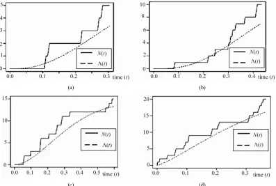
Both the bell-shaped and the beta-shaped intensity are depicted in Figure 1. In Figure 1(a) the claim of occur-rence in the tail of the period, i.e. left and right tail of period, changes slowly. While the beta-shaped intensity is shown in Figure 1(b), the claim of occurrence in the left and right tail of the period changes quickly.
,F P
On a probability space N t
0 d
t
t u u E N t
, is modeled by NHPP with a mean value function or parameter
. As
t
t k t t; 0
; is called the multiplicativeintensity, where
t and k t
N
are defined as the claim intensity rate and the exposure risk, respectively. We consider as a non-decreasing right continuous step function 0 at time t = 0 and jumps of size 1, and
exp ; Pr ! n t tP p N t N t n
n 0,1, 2, n
and for
Pr dN t 1 t dtE dN t
(a) (b)
Figure 1. Non-life insurance claim intensity function, (a) Bell-shaped intensity
t
2 1 8
2
t 42 exp 2π
and (b) Beta-
shaped intensity
t 10 2
t
t
1 4
1 t
t
1 4
,
while p = q.
3. Parameter Estimation of the Non-Life
Insurance Claim Counting Process
In this section, we introduce the methods which are use-ful for parameter estimation of the non-life insurance claim counting process, including the estimating function, the martingale method, and the Bayesian estimation ap-proach (BE).
3.1. Estimating Function
On a probability space F P , where , is
an open interval on the real line, . Sup- pose that the observation , the estimating func-tions, , are functions of and the pa-rameter . By solving
N t ;
N t P p
N t n
;g N t
g N t
;
0
t ;N
, a so-called es- timating equation, an estimate of is obtained. Then
is an unbiased estimating function if
t ;
g N
E g 0 for all (see [9]).
In this study, the estimating function for parameter es-timation of the insurance claim counting process is pro-vided by the martingale method.
3.2. The Martingale Method
The martingales are random processes relating to time. On a probability space
,F P
;t 0
t
0
, we suppose the
in-creasing family t , a filtration or history t, which is the available data at the time . The
proc-ess M
M t t
; is a martingale with respect to if E M t
exist, and
s t
M t
s0
E M t for all . As a result of
the properties of the martingale, E M
0
E M tfor all t 0, then E M
0
0 for a zero meanmar-tingale [10,11].
This study of the martingale method is useful for con-structing an estimating function for a parameter estima-tion of the insurance claim counting process. The process
takes place over a small time interval t t, dt
,
d
dE N t t t t and as a result of the meaning
of martingale property, the martingale can be written as
dN t t dtdM t
0 0
d d d
t t
N u u u M u
, (5) which is a martingale-difference. Then, the following martingale is
, or it can be rewritten in the form of
N t t M t , is a ZMM. Based on ZMM, we
obtain E M t
0 E N t
t
.
0N t t
Thus,
N t
is an estimating equation for parameter estimation of the insurance claim counting process. Also, as a result of the parameter estimate of the process, this can be interpreted as an estimate or, in other words,
t is called the compensator of
N t , and this estimate is useful for predicting the times
of occurrence of insurance claim counts [11]. We can depict the systematic part of the process of insurance claim counts, N t
, related to its compensator,
t
,and the associated martingale N t t M t
t
in Figures 2(a) and (b), respectively, based on a sample of 15 independent random times of claims occurrence in the NHPP with a claim intensity where
2
1 31exp 3
2
t t
.
3.3. A Bayesian Estimation Approach: The Model Specification for the Parameters of Model Claim Intensity
N t ,
In order to get the estimate of the compensator of
ˆ t
(a) (b)
Figure 2. In a sample of 15 independent random times of claims occurrence with the claim intensity
t 2 1 3
2
N t n
, , , , t 31exp
, (a) Non-life insurance claim counting process N(t) related to its compensator Λ(t); and (b) Mar-tingale M(t) = N(t) – Λ(t).
3 3
Gamma ,q c d
c d c2 d2 c d
I(1, ), (8) tion are estimated by the BE. Given , we
sup-pose that 1 2 3 N t are the arrival times of the
claims on the time interval t t t t
0,t
with a cumulative dis-tribution function (a general order statistics model)
1 exp
F t t
exp
n
i tn
. (6) Its likelihood function [4,12] is given by
1 ;
i
l t
, where is a vector of
the parameters of the model claim intensity, denotes the set of claim arrival times, the i of both the bell-
shaped and the beta-shaped intensity function are given
t
*,
in Equations (1) and (2), respectively. While
*, ,p q
of the bell-shaped intensity function and of the beta-shaped intensity function are unknown, the estimate of can be obtained by a Bayesian analysis. The BE approach treats all unknown parameters in Equa-tion (6) as random variables under their prior distribuEqua-tion and derives their conditional distribution upon the known information (sample data of claim arrival times). In this study, we apply the following prior density for
*,
*
1 1 Gamma a b,
2 2
Gamma a b,2
a b2
*, ,p q
* Gamma
2 2
Gamma c d,:
1) ,
2
2) , (7) where a1, b1, and are known parameters, and the following prior density for :
c d1, 1
1) ,
2) p I(1, ),
3)
where 1, 1, , , 3 and 3 are known pa-rameters and Gamma ,
a b denotes a gammadistribu-tion with mean a b and variance a b2
, 1
p q
. The restriction , is imposed with the construct I(1, ). We assume that among parameters, , are independent. The esti-mated parameters are based on the joint posterior density as,
;
h h l , (9)
l
;
h is the joint prior density, and
where is
the likelihood function of . The Equation (9) has a complicated form or no closed form. Therefore, the BE is implemented on the basis of the Markov chain Monte Carlo (MCMC) algorithms with the Gibbs sampler to solve these problems, see [13-16]. In this case, we esti-mate the parameters with the empirical Bayes’ esti-mator obtained by using the BUGS program.
4. Simulation Study
In this study, a simulation model is used to investigate how the observation of the non-life insurance claim counting process can be used to estimate its model pa-rameter, i.e. claim intensity
t or in term
t ,using the estimating function provided by the martingale method with ZMM. In particular, the NHPP of the in-surance claim counts with bell-shaped and beta-shaped intensities, we consider the simulation study of the proc-esses of the insurance claim counts during the claim time interval
0,t
, , , ,
in which the observation involves the claim arrival times, 1 2 3 N t . The claim arrival
times can be simulated by using the mean value function
t t t t
t
, , , ,
E E E E
as a claim arrival time of the HPP with mean one [5]. It implies that 1 2 3 n are independent and
exponentially distributed with mean one, where
Ei ti
ti1 , for all i1, 2,3, , n. So, the nth claim arrival time, tN t n1
1 2
n
t E
, is generated by [5,8]
E E3 En
Ei ofN t
1
, (10) where is the invertible function
t , 0.25
with * 0.1, = and *10, 0.25
,
for the model bell-shaped intensity, a 0.1
and , for the model
beta-shaped intensity.
nd
p q
*
1.25 1.25
p q *10
In this simulation study of the non-life insurance claim counting process over the time interval 0,t
1
c 0.1
, the num-ber of observations, , is composed of 5, 10, 15 and 20. The processes are carried out with 5000 sample paths. In each sample path, the parameter estimate of the model claim intensity is computed using the BE method with the prior distributions given in Equations (7) and (8)
where 1 , , , , 1
N t n
1 0.01
b
0.01
a a25 b2 ,
1 0.1, 2 , 2 , 3
d c 5 d 1 c 5, 3 , and the
mating function, such as the ZMM which is used to esti-mate the parameter of the process (or the com-pensator of ), i.e. fitting the compensator estimate
1
d
t
N t
t
ˆ t to . Also, the mean squared error
(MSE) is provided to measure the fitting
N t
ˆ t
to as the following form
N t
2d
i i
p
u N u u
S 0 1 ˆ MSE t p i
,where Sp denotes the number of sample paths. Notice that the MSE of the compensator estimate ˆ
t offor the processes, as shown in Tables 1 and 2, depends on the parameters of the model claim intensity as in the following results, for the NHPP with a bell- shaped intensity, the parameters of its model claim inten-sity
N t
*
0.1, 0.25
N t
(a small average number of claims over a period), the MSE of the compensator esti-mate of increases as the observation num- ber increases. In the same process with the parameters of model claim intensity
ˆ t
*
10, 0.25
, the MSE of the compensator estimate
t of N t
decreases
ˆ
[image:5.595.306.539.121.230.2]
Table 1. MSE of the compensator estimate ˆ t
of N t
in the NHPP of the non-life insurance claim counts with bell-shaped intensity.*
N t MSE
0.1 0.25 5
10 15 20 0.873166 1.663399 2.428750 3.141596
10 0.25 5
[image:5.595.55.288.625.736.2]10 15 20 5.968821 5.676725 4.630684 4.880201
Table 2. MSE of the compensator estimate ˆ
t of N t
*
in the NHPP of the non-life insurance claim counts with beta-shaped intensity.
pq
N t MSE
0.1 1.25 5
10 15 20 0.877067 1.883131 2.821956 4.170855
10 1.25 5
10 15 20 0.885957 1.971573 4.469941 5.246322
while its observation number increases until the observed 15 times of claims occurrence, and then its MSE values begin to increase as the observation number increases. For the NHPP with a beta-shaped intensity * 0.1,
1.25
p q
* 10, (a small peak level for claim intensity) and 1.25
p q
, the MSE of the compensator
estimate ˆ
t of N t
N t
increases exponentially as their observation number increases.
Some examples in these situations of the NHPP with both bell-shaped and beta-shaped intensities, of non-life insurance claim counts based on a sample of 5, 10, 15 and 20 times of claims occurrence, are illustrated in Fig-ures 3 and 4, including the and its compensator
t
*=10
0.25
. Figure 3 shows a sample path of the process with a bell-shaped intensity , . The N t
and its compensator
t*=10
0.25
are characterized by the pa-rameters of model claim intensity , , the compensator
t N t
*=10
N t
fits well with , as the ob-servation number is 15 and 20 (slightly larger than the claim intensity ). While the and its com-pensator
t*=10
p q 1.25
in the process with a beta-shaped inten-sity , is shown in Figure 4, the compensator
t fits with N t
, as the observationnumber is small.
5. Conclusions and Discussion
5.1. Conclusions
In a non-life insurance claim counting process over the time interval
0,t
, the simulation study of the NHPPwith both bell-shaped and beta-shaped intensities dem-onstrates the fitting of the compensator estimate ˆ
tto N t
*
. The model fitting depends on the parameters of model claim intensity and model specification of claim intensity. Firstly, regarding the NHPP with the parameters of the model bell-shaped intensity, a has almost no claim occurrences over a period and any The compensator estimate ˆ
t is a good fit to N t
*
with small MSE and small number of observations. In the same process with the parameters of the model claim
ntensity, an average number of claims over a period
i
201 OJS
(a) (b)
[image:6.595.98.502.86.337.2](c) (d)
Figure 3. N(t) and its compensator Λ(t) in the NHPP with the parameters of a bell-shaped intensity λ* = 10, σ = 0.25 based on a sample of (a) 5 claims; (b) 10 claims; (c) 15 claims; and (d) 20 claims.
(a) (b)
(c) (d)
Figure 4. N(t) and its compensator Λ(t) in the NHPP with the parameters of a beta-shaped intensity λ* = 10, p = q = 1.25 based on a sample of (a) 5 claims; (b) 10 claims; (c) 15 claims; and (d) 20 claims.
Copyright © 2 SciRes.
is not less than one and any . The MSE of the com-pensator estimate of is small while the number of observations is slightly larger than the value of
ˆ t N t
*
. Secondly, when the model beta-shaped intensity
is considered with the parameters , the compensa-tor estimate
pq
ˆ t is a good fit toN t
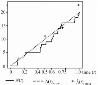
with small [image:6.595.101.498.378.645.2]Figure 5. N t
, ˆ
t NHPP, and ˆ
t CRED in the NHPP with a bell-shaped intensity of non-life insurance claim counts.by a sample path relating N t
t . and its compensator
5.2. Discussion
This study is a parameter estimation approach to non-life insurance claim counting process. The parameter
t
of the claim counting process is estimated from observa-tions using an estimating function, such as ZMM. A re-sult of the parameter estimate ˆ t
N t
can be interpreted as an , called the compensator estimate ˆ
t
N t
tN t
of . This estimate is also useful for predicting the time of insurance claim occurrences. Using an example, we can depict a comparison of the two approaches of non- life insurance claim counts, including this insurance claim counting process and the Jewell’s credibility ap-proach. In Figure 5, the compensator NHPP in the NHPP with a bell-shaped intensity (dashed line) is a good fit to over time
ˆ
0,t
; on the other hand, the procedure of the credibility estimate CRED (+) or the compensator CRED of on the credibility model does not consider the behavior of insurance claim counts over time.
ˆ t
ˆ t
N t
REFERENCES
[1] W. S. Jewell, “Credible Means Are Exact Bayesian for Exponential Families,” ASTIN Bulletin, Vol. 8, No. 1, 1974, pp. 77-90.
[2] R. Kaas, D. Dannenburg and M. Goovaerts, “Exact
Credibility for Weighted Observations,” ASTIN Bulletin, Vol. 27, No. 2, 1997, pp. 287-295.
doi:10.2143/AST.27.2.542053
[3] E. Ohlsson and B. Johansson, “Exact Credibility and
Tweedie Models,” ASTIN Bulletin, Vol. 36, No. 1, 2006, pp. 121-133. doi:10.2143/AST.36.1.2014146
[4] T. Mikosch, “Non-Life Insurance Mathematics,” 2nd
Edition, Springer-Verlag, Berlin, 2009. doi:10.1007/978-3-540-88233-6
[5] M. Morales, “On a Surplus Process under a Periodic En- vironment: A Simulation Approach,” North American Ac- tuarial Journal, Vol. 8, No. 2, 2004, pp. 76-87.
[6] Y. Lu and J. Garrido, “Doubly Periodic Non-Homogen- eous Poisson Models for Hurricane Data,” Statistical Me- thodology, Vol. 2, No. 1, 2005, pp. 17-35.
doi:10.1016/j.stamet.2004.10.004
[7] J. Garrido and Y. Lu, “On Double Pariodic Non-Homo- geneous Poisson Processes,” Bulletin of the Association of Swiss Actuaries, Vol. 2, 2004, pp. 195-212.
[8] U. Jaroengeratikun, W. Bodhisuwan and A.
Thong-teeraparp, “A Statistical Analysis of Intensities Estima-tion on the Modeling of Non-Life Insurance Claim Counting Process,” Applied Mathematics, Vol. 3, No. 1, 2012, pp. 100-106. doi:10.4236/am.2012.31016
[9] P. Mukhopadhyay, “An Introduction to Estimating Func-tions,” Alpha Science International Ltd., Harrow, 2004. [10] P. K. Andersen, O. Borgan, R. D. Gill and N. Keiding,
“Statistical Models Based on Counting Processes,” Sprin- ger-Verlag New York, Inc., New York, 1993.
[11] P. Yip, “Estimating the Number of Error in a System Using a Martingale Approach,” IEEE Transactions on Reliability, Vol. 44, No. 2, 1995, pp. 322-326.
doi:10.1109/24.387389
[12] J. E. R. Cid and J. A. Achcar, “Bayesian Inference for Nonhomogeneous Poisson Processed in Software Reli-ability Models Assuming Nonmonotonic Intensity Func-tions,” Computational Statistics & Data Analysis, Vol. 32, No. 2, 1999, pp. 147-159.
doi:10.1016/S0167-9473(99)00028-6
[13] J. Gill, “Bayesian Methods: A Social and Behavioral Sci- ences Approach,” Chapman and Hall/CRC, London, 2008.
[14] T. Hirata, H. Okamura and T. Dohi, “A Bayesian Infer-ence Tool for NHPP-Based Software Reliability Assess-ment,” In Y. H. Lee, T.-H. Kim, W.-C. Fang and D. Slezak, Eds., Lecture Notes in Computer Science, Vol. 5899, Springer, Berlin, 2009, pp. 225-236.
[15] D. P. M. Scollnik, “Actuarial Modeling with MCMC and BUGS,” North American Actuarial Journal, Vol. 5, No. 2, 2001, pp. 96-124.