ISSN Online: 2152-2219 ISSN Print: 2152-2197
DOI: 10.4236/jep.2018.99062 Aug. 31, 2018 991 Journal of Environmental Protection
Agent-Based Modeling: An Application to
Natural Resource Management
Inocencio Rodríguez González, Gerard E. D’Souza, Zarina Ismailova
College of Agriculture and Human Sciences, Prairie View A&M University,Prairie View, TX, USA
Abstract
Computer programs have been categorized as a useful tool to evaluate the complexity of systems. In fact, agent-based modeling (ABM) is considered a new method to model complex systems characterized by the role of indepen-dent and interrelating agents. Simulations contribute in estimating and com-prehending emerging behaviors that require the development of new regula-tions for local agents that would make improvements to the system. This pa-per offers an example of a methodology and a process utilized to develop a simulation model named Befergyonet, an ABM used to conduct computer simulations within a spatio-intertemporal environment. The methodology discussed in this paper is intended solely to stimulate the use of innovative computer programs to simulate complex systems as an approach to represent real world events and may be a methodological guide for readers interested in developing their own ABM.
Keywords
Agent-Based Modeling, Dynamic Systems, Environmental Economics, NetLogo, Simulation
1. Introduction
As real-life systems become more complex, so do the analytical techniques ne-cessary to assess and simulate them. Agent-based modeling (ABM) is one such technique. ABM is defined as a number of virtual individuals (or “agents”) inte-racting in an “artificial, experimenter-controlled environment” [1]. By enabling researchers to simulate an environment in which the agents or key players in a system can explicitly interact with their surrounding environment, enables us to better understand the system and manipulate it to achieve planning and policy How to cite this paper: González, I.R.,
D’Souza, G.E. and Ismailova, Z. (2018) Agent-Based Modeling: An Application to Natural Resource Management. Journal of Environmental Protection, 9, 991-1019. https://doi.org/10.4236/jep.2018.99062
Received: December 19, 2018 Accepted: August 28, 2018 Published: August 31, 2018
Copyright © 2018 by authors and Scientific Research Publishing Inc. This work is licensed under the Creative Commons Attribution International License (CC BY 4.0).
http://creativecommons.org/licenses/by/4.0/
DOI: 10.4236/jep.2018.99062 992 Journal of Environmental Protection goals. Planners must develop systems that function harmoniously not only in-ternally but also with the environment that they are projected to match. A sys-tem can be described as a region, an individual, a herd of animals or a nation while a subsystem is expressed as explanatory variables which might be common to some subsystems or restricted to a subsystem. When developing the model, it is important to identify first the calculations or simultaneous equations under consideration since they will be used by the computerized system.
Our agent-based model is more focused on optimizing resources available in a spatial domain in order to intensify the benefits that a diversified industry would bring to the region. For the ABM, the NetLogo platform is employed to simulate the effects of a diversified industry that enhances the environment and society as well as profitability when resources are optimized. Through our model we pro-pose making comparisons between specialized and diversified enterprises to evaluate profitability and the resulting environmental implications within a re-gion for clustering systems. Indeed, economies resulting from clustering and ag-glomeration are considered in this study as an important element of a sustaina-ble production system. In our model (BET), we define a diversified operation as the farm of interest within the pasture-based beef (PBB) industry with the goal of generating income from beef, energy and carbon offset sales. In contrast, the specialized operation is focused solely on beef production and without explicit recognition of any clustering effect. The main purpose of this paper is to illu-strate the application of agent-based modeling and simulation as a cost-effective decision-support and policy tool compared to surveys or experiments.
2. Background
2.1. Agent-Based Models
DOI: 10.4236/jep.2018.99062 993 Journal of Environmental Protection of a system; and 3) ABM is flexible. It is clear, however, that the ability of ABM to deal with emergent phenomena is what drives the other benefits [6]. The use of ABM is quite versatile and extends to a variety of different settings, ranging from health care [7] to aerospace [8]. However, the spatio-intertemporal ap-proach used here is relatively unique among known applications of ABM.
2.2. Model Development
Different simulation models have been developed through computer networks to evaluate real world problems under specific scenarios in order to approach the potential solutions that can be used by business, industry, and/or policy-makers. Planners must develop systems that function harmoniously not only in-ternally but also within the environment that they are projected to model. A sys-tem can be described as a region, individual, a herd of animals or a nation, while a subsystem is expressed as explanatory variables which might be common to some subsystems or restricted to a subsystem. It is also crucial that models do not violate the assumptions under consideration. In order to simulate manage-ment systems for a particular set of social, economic and production scenarios, maximization skills must be taken into account [9]. When developing the model, it is important to identify first the calculations under consideration since they will be used by the computerized system. Also, theory, data and program are fundamental in agent-based computer simulation models [3]. Moreover, the ex-tendibility of the model is essential for future research purposes since potential users are likely to adapt the model for new applications. This way, an investiga-tor would be able to use an existing model to add a new characteristic in order to find an answer while others may want to adapt the model to better suit their purpose [10].
2.3. Language Programming
DOI: 10.4236/jep.2018.99062 994 Journal of Environmental Protection particular species while still others consider different species, and the conse-quences of foraging. Since simulation results are the end point of the functions developed for the model, they must be cautiously interpreted. The necessity of conducting production research can be replaced by effective models that simu-late production [9]. For instance, Carter, along with the US Geological Survey, developed a spatially-explicit model of animal behavior, in which pasture con-sumption and animal movement were jointly analyzed [4].
2.4. Platform Considered
Since the focus of this study is on simulations using an ABM known as NetLogo, it is significant to point out some of its features for a basic understating of the program. This is a free of charge model developed by Northwestern University and suitable for developing complex systems. It provides manuals, dictionary, tutorial and other mechanisms to help users in the development process. Net-Logo provides different alternatives in which the system that needs to be ex-plained can be built up. For instance, the simulation can be performed by adding the codes in the procedures tap and linking them to functional features such as buttons, sliders, monitors, and switches among others available in the interface tab which allow the simulation to begin and stop as well as to modify the condi-tions or parameters of the system. Simulacondi-tions can also be done by intercon-necting a system dynamic diagram with the codes developed in the procedures tab and with the interface functional features. Depending on the programmer’s approach, the system behavior could also be graphically illustrated or viewed in what is called the “view or world window” that is based on coordinates and the codes expressed in the procedures tab in which the boundaries and topology of the world are defined.
3. Befergyonet Model
3.1. An Overview
BET is a simulation model based on agent-based modeling that permits the evaluation of PBB and renewable energy production as well as carbon offsets as a function of environmental variables from a deterministic and stochastic perspec-tive. The model also employs R-extension as a tool to conduct statistical analysis developed by [11]. BET allows an approach to compare potential beneficial en-vironmental effects as well as profitability under certainty and uncertainty. The model is composed of two key elements: the supply and the environmental and economic impacts interconnected through high quality beef, renewable energy and carbon dioxide emissions reduction within a specific region simulating the interaction among agents spatially distributed bringing some economic and en-vironmental implications to the whole system.
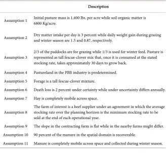
DOI: 10.4236/jep.2018.99062 995 Journal of Environmental Protection during the winter season (November to April). The association among methane emissions and CO2 arises from the fact that methane has 25 times the global warming capacity of CO2; however, when one ton of methane is utilized for energy production, it releases one ton of carbon dioxide. This implies that burning one ton of methane is equal to reducing twenty four tons of CO2 [12]. Thus, the equivalence to CO2 emissions in terms of methane is called carbon dioxide equivalent (CO2e) emissions. Furthermore, our model interconnects the benefits and costs associated with PBB and renewable energy production and subsequently carbon reductions by maximizing the pasture available in a specific region among farms within a radius of distance in a planning horizon of 15 years under certain and uncertain conditions. BET is an experimental approach that also evaluates potential clustering development in which resources available such as cattle, forage allowance and manure generated within the sector are optimized within a spatially interconnected industry on a yearly basis. We employ 11 as-sumptions throughout this experimental approach as describe in Table 1.
[image:5.595.210.541.423.725.2]This ABM is composed of pre-interaction and interaction stages. During the pre-interaction stage, the model simulates pasture growth as a function of daily irradiance, rainfall and temperature as well as latitude based on historical data for 15 years for the deterministic and stochastic approaches in order to obtain the control variable or the optimal stocking rate per year over the entire spatial domain. During the interaction phase, the interactive world becomes active and
Table 1. Assumptions.
Description
Assumption 1 Initial pasture mass is 1,400 lbs. per acre while soil organic matter is 6800 Kg/acre.
Assumption 2 Dry matter intake per day is 3 percent while daily weight gain during grazing and winter season are 1.5 and 0.87, respectively.
Assumption 3 2/3 of the paddocks are for grazing while 1/3 is used for winter feed. Pasture is represented as tall fescue-clover mix that, once it is consumed at the stated stocking rate, takes approximately 30 days to grow back.
Assumption 4 Pastureland in the PBB industry is predetermined. Assumption 5 Forage is a tall fescue-clover mixture.
Assumption 6 Death loss is 2 percent under certainty while under uncertainty differs annually. Assumption 7 Hay is completely mobile across space.
Assumption 8 The farm of interest is a beef supplier under an agreement in which the average stocking rate over the planning horizon is the minimum stocking rate to be sold at the end of each operational year.
Assumption 9 The slope in the contracting farm is flat while in the nearby farms might differ. Assumption 10 90 percent of the manure in the spatial domain is recoverable.
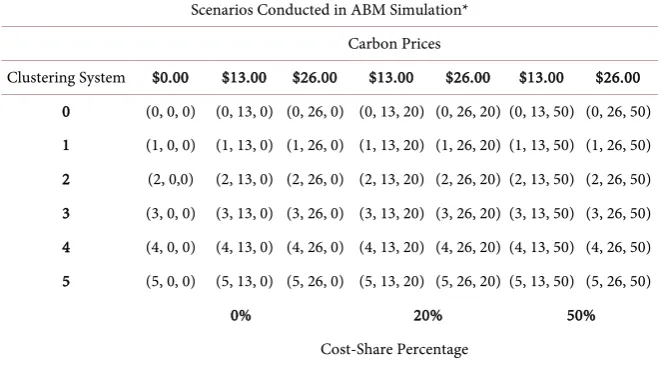
DOI: 10.4236/jep.2018.99062 996 Journal of Environmental Protection the interaction among agents takes place generating emerging patterns and data based on their rational behavior. In fact, the model is designed to be run for a total of over 10,900 iterations repeated from 5 to 10 times for each scenario exer-cised in order to obtain a fair variability from the stochastic simulation. We em-ployed a total of seven scenarios in which every scenario (under the exis-tence/absence of carbon prices and cost-share programs) was tested under six hypothetical clustering systems, specifically from zero to five clustering members as depicted in Table 2.
This simulation experiment was designed to evaluate potential influences from a diversified pasture-fed industry in most counties in WV based on data available as a representation of the Appalachian region. We used Monongalia County for the different scenarios exercised on this simulation; however, the model can be run for any other county to simulate the potential impacts for the proposed industry on each county.
[image:6.595.209.540.527.710.2]NetLogo allows choosing important elements such as stocks, variables, flows and links to perform the simulation in a dynamic format [13]. For instance, each of these elements is identified and linked to each other so it simulates the va-riables that influence the flows that eventually reduce or increase the stocks val-ues over time. In this model, the daily pasture growth and forage available for grazing and hay, beef production, electricity generation from anaerobic digester, manure production, carbon offset and CO2 baseline have been categorized as stocks. On the other hand, some variables are represented as values or expres-sions that would have an effect on inflows and outflows (represented as pipe-lines) and available through arrows in the system dynamics modeler. In this model, environmental as well as economic variables are integrated in the system dynamics as a form of extraction rates such as forage intake and carbon offset rate as well as costs and net present values associated with the daily interactions. The advantages of this agent-based software consist of: 1) the capability to
Table 2. Scenarios.
Scenarios Conducted in ABM Simulation* Carbon Prices
Clustering System $0.00 $13.00 $26.00 $13.00 $26.00 $13.00 $26.00 0 (0, 0, 0) (0, 13, 0) (0, 26, 0) (0, 13, 20) (0, 26, 20) (0, 13, 50) (0, 26, 50) 1 (1, 0, 0) (1, 13, 0) (1, 26, 0) (1, 13, 20) (1, 26, 20) (1, 13, 50) (1, 26, 50) 2 (2, 0,0) (2, 13, 0) (2, 26, 0) (2, 13, 20) (2, 26, 20) (2, 13, 50) (2, 26, 50) 3 (3, 0, 0) (3, 13, 0) (3, 26, 0) (3, 13, 20) (3, 26, 20) (3, 13, 50) (3, 26, 50) 4 (4, 0, 0) (4, 13, 0) (4, 26, 0) (4, 13, 20) (4, 26, 20) (4, 13, 50) (4, 26, 50) 5 (5, 0, 0) (5, 13, 0) (5, 26, 0) (5, 13, 20) (5, 26, 20) (5, 13, 50) (5, 26, 50)
0% 20% 50%
Cost-Share Percentage
DOI: 10.4236/jep.2018.99062 997 Journal of Environmental Protection integrate routines written in Java language into the model and synchronize lan-guage programming with the systems dynamic modeler; 2) the capability to pro-vide instructions to users before, during, and at the end of the simulation; 3) the availability to illustrate the interaction among agents and space through graphs as well as visual representation; 4) the flexibility to export simulation results in different file extensions such as txt and csv for further analysis in other programs as well as during the simulation in its interface view; 5) the ability to develop a control panel to manipulate the initial conditions and parameters of the model; 6) the advantage of importing data to be used in the simulation; 7) flexibility of using extensions (BET employs R-extension) to perform statistical instruments during the simulation.
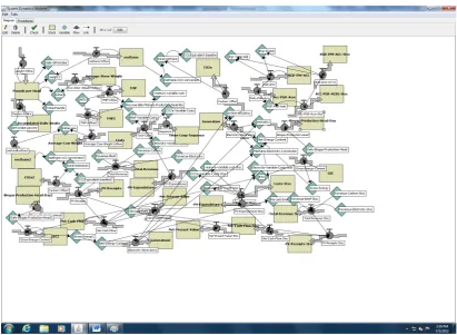
In our approach, a system dynamic modeler was developed in order to cap-ture the dynamics over time and space expressed through mathematical equa-tions using NetLogo. Figure 1 and Figure 2 present the system dynamic mod-eler of the concept proposed. In the system dynamic diagram, links allow a value from a variable or stock into a stock or flow making them available from one source to another in order to perform the simulation [13]. As we can appreciate in Figure 1, the largest rectangular boxes represent the stocks that are influenced by the pipeline-shapes that store equations composed of values located either in the code tab, the interface view or in the variables presented as green rectangular boxes (smaller boxes) in the diagram while the arrows or links connect values among the previously explained components. Note that some variables are con-nected to more than one arrow when variables are used in other functions al-lowing for multi-use and eliminating unnecessary replications of the same varia-ble in the system such as the “Pgr-Temp-Adj” variavaria-ble that is used by “RGR-ENV” and “RGR-ENV-STOC” depicted in Figure 1.
The stocks are able to change over time due to the influences caused by changes on their flows. The flows are affected by changes in the values of their variables and time making the stocks either to increase or decrease over time. These variables might be identified as a parameter or value stored in the variable or identified in the interface view under the simulation control panel. Thus, the interactions taking place in the whole system would basically have an impact on stocks that eventually will be reflected on production, profitability among other components of the system. Figure 2 shows a closer view of one of the segments represented in the complete flowchart or diagram.
DOI: 10.4236/jep.2018.99062 998 Journal of Environmental Protection
Figure 1. NetLogo-System Dynamics Modeler Used for Simulation: Complete Flowchart. The figure above shows the system dynamic modeler used in BET model. The largest rectangular boxes represent the stocks that are influenced by the pipeline-shapes that store equations composed of values located either in the code tab, the interface view or in the variables presented as green rectangular boxes in the diagram while the arrows or links connect values among the previously explained components. Note that some of variables are connected to more than one arrow since that variable might be used in other functions. Figure 2 shows a segment of the complete flowchart for a more specific explanation.
[image:8.595.223.524.471.594.2]DOI: 10.4236/jep.2018.99062 999 Journal of Environmental Protection
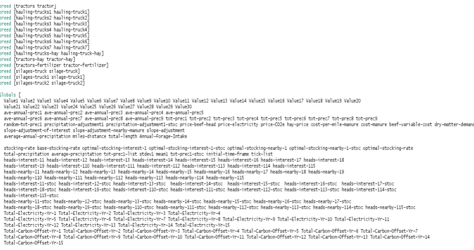
Figure 3. NetLogo-Programming Language in Java. Note: In the coding section, the interacting elements of the “world” such as agents and global variables among other components are created and synchronized with the system dynamics modeler.
3.2. Experimental Model: Agents, System and Interactions
3.2.1. World
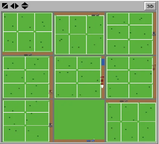
The NetLogo simulated world consists of a 49 by 49 grid of coordinates with a patch size of 3 (world landscape) in which agents (“turtles” and “patches”) inte-ract based on the resources available throughout space. In our ABM, dynamic and static agents are identified as farmers, farms, stocking rates, vegetation, tractors, manure storage, anaerobic digesters, manure transporters, silage haul-ing trucks, pasturelands (green) and roads (gray). The interaction among these agents on the system is eventually reflected in the production of final products as well as returns to the farm of interest. In fact, it is intended to simulate a realistic model of plan-animal interaction based on entrepreneur decisions within an emerging PBB industry.
3.2.2. Farm Locations and Farmers
DOI: 10.4236/jep.2018.99062 1000 Journal of Environmental Protection
Figure 4. Interactive World in NetLogo.
when the clustering system is activated. On the other hand, the model also si-mulates farmers’ interaction with the livestock during the grazing season by ro-tating it from one paddock to the next within an intertemporal context. This in-teraction provides a close to reality representation of a PBB industry where the land resources are optimized. This occurs when the forage system fits with the total amount of livestock as an approach to undertake appropriate pasture man-agement techniques [15].
3.2.3. Stocking Rate
DOI: 10.4236/jep.2018.99062 1001 Journal of Environmental Protection cattle suppliers each year.
The stocking rate is derived during the first stage of the simulation and ran-domly distributed on paddocks by the farmer during the second phase of the modeling. During the grazing season, animals are rotated between paddocks for optimal forage consumption. After reaching approximately 900 lbs. In April, when the animals are sold for slaughtering, a new stocking rate is introduced to begin the annual operational cycle over again. It is important to mention that beef prices are seasonal which tends to reach the highest during April compared to October with a difference of approximately 5 percent [23] making appealing to beef producers to sell during this particular season. However, our approach employs annual average prices.
1) Manure Hauling Trucks. These trucks simulate the manure haulers trans-porting the manure from adjacent cow/calf farms to the farm of interest during the winter season. The manure collected during this period of time is used to generate electricity and carbon offsets in the contracting business.
2) Silage Transporters. These trucks simulate silage transportation from the closest silage supplier to the farm of interest and nearby stocker farms. This oc-curs when the forage production on these farms are limited to satisfy the amount of animals purchased on an annual basis.
3) Carbon Offset Counter. It is a static agent with the purpose of explicitly il-lustrating the amount of the current CO2 equivalent reductions that have been reduced during the winter season. Although this static agent does not move, it indeed depends on the carbon offset stock developed in the system dynamics modeler for execution.
4) Lagoon. This static agent simulates a manure lagoon or pond to explicitly show the CO2e baseline that would be generated from manure during the winter season if it were deposited into a pond instead of using it for electricity genera-tion. This agent depends on CO2e emissions generated in the system dynamics. 5) Manure Collection Counter. This agent is the manure storage in the farm of interest. This is another static agent with the main function of illustrating the amount of manure collected during the winter season in the interacting world.
6) Anaerobic Digester. This agent represents the daily electricity generated from the manure collected during the winter season. This agent is located at the contracting farm in the simulated world.
7) Paddocks. Paddocks play an essential role in the PBB industry since it con-tributes in optimizing the amount of pasture available. In other words, they represent the grazing area in which animals are exposed to a natural environ-ment for approximately 180 days.
8) Pasture. The forage is represented through green patches that interact with the stocking rate when consumed. In our model, pasture is represented as tall fescue-clover mix that, once it is consumed at the stated stocking rate, takes ap-proximately 30 days to grow back.
DOI: 10.4236/jep.2018.99062 1002 Journal of Environmental Protection their inputs from nearby farms to the farm(s) making the request for beef and electricity production. These are basically patches designed to represent the pathways for the mobilization of the resources needed within the region.
10) Winter Building. The structure in which the stocking rate is placed for the winter season is fed with forage. Also, it is the location for manure collection which is transferred to the adjacent anaerobic digestion system.
11) Trees. This simulates the typical surrounding vegetation in a PBB farm representing seasonal changes during an operational year. As a result of inter-temporal changes, trees change color as a representation of the four seasons in WV based on current temperature.
12) Links. Links are useful agents with the main purpose of connecting the clustering system during simulation. They also measure the average distance in miles among the members of the cluster during the interaction phase.
13) Silage Tractors. These tractors simulate hay collection for winter season. They collect forage only on 1/3 of the total acreage or 2 paddocks out of the 6 paddocks in which the area is fertilized approximately a month before pasture collection. Also, these agents are invoked by the farm of interest at the end of Spring and Summer seasons every year throughout the planning horizon.
14) Fertilizer Applicators. It is assumed that the fertilization season starts in April at a rate of two paddocks per month. This agent is also invoked by the farm of interest and takes place during the interaction stage.
15) Cattle Hauling Trucks. These trucks simulate the supply of cattle from the cow/calf farms to the farm of interest. This event occurs at the beginning of each operational year before grazing season starts.
3.2.4. Selections: Buttons, Choosers, Switches and Monitors
1) Buttons. The first buttons under the “Simulation Control Panel” (SCP) are categorized as “System Setup”, “Simulation” and “Simulation by Step”. They have been designed to setup and refresh the initial conditions, run the simula-tion continuously until reaching the planning horizon and run the model step by step or one iteration at the time.
2) Clustering System. The model allows selecting the composition of the clus-tering system for manure supply by changing the number of farms in the system from the chooser “Clusters” under the SCP. This allows users to perform the si-mulation under different clustering systems for sensitivity analysis generating some economic and environmental impacts within the region. It allows users to select from 0 to 5 clusters to simulate their interaction and their influences within the system or world.
DOI: 10.4236/jep.2018.99062 1003 Journal of Environmental Protection have the option to select 0.4, 0.5, 0.8, 1 or 1.2 to represent an approximation of 15, 20, 30, 40 or 50 radius mile distance between farms, respectively.
4) County Selection. The “Country-WV” permits county selection to execute the simulation based on specific county data in order to identify the potential environmental and economic impacts in a specific region. Due to lack of data, most of the counties in WV can be simulated in BET.
5) Initial Weight. The “Initial-Weight” option allows selecting the initial weight per head at time zero. In this experimental study, we define 500 lbs. as the initial weight based on a survey conducted of farmers in the pasture-fed beef industry at the national level [22] and reach a final weight of approximately 900 lbs. at harvest. However, this chooser permits users to select an initial weight between 400, 450, 500 or 550.
6) Carbon Price. The “Carbon-Prices-List” provides a list of the commonly used carbon prices [12] [25] in order to perform a sensitivity analysis based on changes in carbon prices assuming the existence of a carbon market. In fact, it is expected that pressure to decrease greenhouse gas emissions could begin in-creasing in the future; therefore, carbon prices would eventually rise significant-ly. However, uncertainty still exists with regard to the carbon offset market in a cap-and-trade framework [12]. This is one of our parameters for policy recom-mendations.
7) DM-Intake-List. Although our default dry matter intake is 3 percent, BET provides the option of changing this percentage. This was done for the benefit of prospective users of the model providing some flexibility in simulation perfor-mance.
8) Switches. Switches displayed in the SCP, like for example, “Show-Weight?”, “Show-Manure?”, “Show-CO2-Baseline?”, “Show-CO2-Offset?”, “Show-Electricity?” and “Show-Profitability?” are used to either activate or deactivate stocking rate weight, manure production, CO2 baseline generation, carbon offset, electricity production on a daily basis while the business economic performance is shown at the end of the simulation, respectively. The values are explicitly presented as tags or labels in some of the dynamic (animals) or static (manure storage, anae-robic digester, pond or manure lagoon and the carbon offset counter) agents while the interaction is simulated.
DOI: 10.4236/jep.2018.99062 1004 Journal of Environmental Protection the Web Soil Survey [26]. In this model, we use the average slope which is prompted through the SLOPE-ADJUSTMENT variable in BET based on coor-dinates identified on the Web Soil Survey and monitored under the “Terrain Slope” section in the interface view. The sloping factor is based on slope ranges for specific locations in which slopes within ranges between zero to ten percent, eleven to thirty and thirty one to sixty are adjusted as 1.0, 0.7 and 0.3, respec-tively. Furthermore, the death loss percentage is monitored under both certainty and uncertainty simulations. The county location is also displayed through the “Latitude” monitor under the “County Selection”.
10) Cost-Share Program. The “Cost-Share-Program” selection provides a list of percentages that can be hypothetically considered as a policy development tool in order to share the costs associated with the initial capital investment needed to afford the anaerobic digester in the PBB industry. This allows users to choose from different cost-share options, especially when conducting sensitivity analysis toward profitability.
4. Outcome from Emerging Patters: Results Generation
Besides the interaction within the system illustrated in the interactive world, BET has been conveniently programmed to provide simulation results in several forms.1) Plots. Plots are graphical representations of the system interaction in which stocking rate, pasture growth rate and average temperature and precipitation rate and depicted over time during the first simulation stage. Others plots are il-lustrated such as daily beef production, renewable energy generation and carbon offset as well as CO2 emissions during the second phase of the simulation per-formance.
2) Output. The model also provides results of the stocking rate based on the system interaction in the interface window below the “Simulation Results” box during the two phases of the simulation. Although complete outcomes are stored in a spreadsheet, this allows users to have a quick view of some of the results.
3) Total Outcomes. Outcomes from the ABM can also be exported to a spreadsheet for further evaluation once the simulation is completed. This way, a more comprehensive database is generated that can be accessed through a pro-gram such as MS-Excel for comparison purposes and further analysis. In order to perform this task, a window providing instructions appears before the simula-tion takes place right after the “System Setup” button is clicked. After this task has been executed, it is just a matter of choosing the conditions explained under section “Selections” and by clicking either “Simulation” or “Simulation by Step” button to perform the simulation.
5. Simulated Equations and Assumptions
DOI: 10.4236/jep.2018.99062 1005 Journal of Environmental Protection used for the simulation illustrated below. However, the Java code or language program developed in NetLogo provides complete information of the entire combination of equation and the code required to perform the simulation. The complete model has also been made available at the NetLogo User Community Models website at
http://ccl.northwestern.edu/netlogo/models/community/BEFERGYONET%20M ODEL as a contribution for researchers and other parties interested in either us-ing, extending or learning more about the model.
As an initial condition at time zero, we are assuming that an initial pasture mass is 1400 pounds per acre [17] [27] while the soil organic matter value has been identified as 6800 Kg/acre. As a way of simplifying the complexities de-scribed in our theoretical approach, our soil organic matter assumption is based on a 2 inches soil layer with a 3 percent organic matter in which 58 percent is composed of carbon or 7900 Kg [28]. In fact, under acceptable management practices, state variables would reach equilibrium when the control variable is under optimal conditions and the time horizon is sufficient. In other words, the system is intended to reach a productive pattern that can be sustained by keep-ing it under a stable operation [29]. Nonetheless, the use of manure as fertilizer may differ among the literature reviewed. For instance, the implications of using tall fescue grass and clover mix as the primary diet for animals might require approximately 200 lbs. per acre on an annual basis [30] [31] to assure the nu-trients needed in the soil for plant growth. In fact, the percentage composition of manure produced by beef cattle is typically 0.54, 0.18 and 0.39 with an approxi-mation of 3:1:2 in terms of nitrogen (N), phosphorus (P) and potassium (K) (Rayburn et al., 2006). On the other hand, approximately 1025 pounds per acre of biosolids from anaerobic digestion systems can be applied in tall fescue fields [32]. Thus, in order to assure that the pasturelands acquire the necessary nu-trients, 620 pounds of digested manure are applied per acre annually which might not a limitation since in the contracting farm over 1500 lbs. is produced per head annually.
Assumption 1: Initial pasture mass is 1400 lbs. per acre while soil organic matter is 6800 Kg/acre. In our approach is also assumed that the daily pasture intake per head is 3 percent of its body weight [14] [16] [17] with a daily weight gain of 1.5 and 0.87 pounds on a daily basis during grazing and winter seasons, respectively [18] [19] [20]. Furthermore, the livestock grazes 2/3 of the paddocks while 1/3 is used for hay or silage for winter feed each year based on expert opi-nion.
Assumption 2:Dry matter intake per day is 3 percent while daily weight gain during grazing and winter season are 1.5 and 0.87, respectively.
Assumption 3:2/3 of the paddocks are for grazing while 1/3 is used for win-ter feed.
DOI: 10.4236/jep.2018.99062 1006 Journal of Environmental Protection
5.1. Pasture Growth
The pasture growth equation is a dynamic equation intended to estimate relative plant growth rate of forage crops based on daily solar radiation, precipitation events, coordinates as well as minimum, average and high temperatures simu-lated in NetLogo based on expert opinion (Ed Rayburn, Forage Extension Spe-cialist, West Virginia University) [33] [34] [35]. This equation is crucial in our simulation model since the optimal consumption of the pasture available mainly determines the optimal stocking rate for each year and eventually, beef and elec-tricity production as well as a carbon offset. In addition, our simulation consid-ers a rest interval of approximately 30 days for tall fescue-clover mix to regrow after grazing as well as silage collection [17] [30] since “erect-growing forage species” have been identified as best to be used also for silage or hay due to their high yield potential [36] which are frost seeded every three years in order to supply a considerable component of the cattle’s diet. In fact, a survey conducted of PBB producers at the national level identified cool season grass-clover as an extremely important component of the forage system [22]. Furthermore, studies in which the grass-legume mixture as tall grass-clover has been compared to other grass-legume mix (tall-grass alfalfa and bluegrass-clover), have demon-strated that tall grass-clover presents faster growth rate on average than other mixtures [37]. In BET, every farm in the spatial domain relies on 93 acres of pastureland which is divided into 6 paddocks [14].
Assumption 4:Pastureland in the PBB industry is predetermined. Assumption 5:Forage is a tall fescue-clover mixture.
Daily PA RGR ENV RGR MAX= ∗ (1)
The daily pasture growth rate per acre (Daily PA) is defined as relative growth rate associated with the total environmental interaction (PGR ENV) times the expected maximum pasture growth rate (PGR MAX) in which PGR MAX is as-sumed to be constant with a value of 60 (lbs./acre).
2
RGR ENV RGR TEMP RGR DL RGR H O= ∗ ∗ (2)
The RGR ENV depends on the relative growth rate due to mean air tempera-ture (RGR TEMP) times relative growth rate based on day length multiplied by expected maximum pasture growth rate (PGR MAX) and the relative growth due to available soil water (RGR-H2O) in which RGR TEMP is defined as fol-lows:
If TAVE < UPCT; then
(
)
(
)
RGR TEMP UPCT TAVE 1 UPCT UPOT= − ∗ − (3)
where UPCT is defined as Upper Critical Temperature and UPOT is as Upper Optimum Temperature.
DOI: 10.4236/jep.2018.99062 1007 Journal of Environmental Protection On the other hand, if TAVE < LOPT (Lower Optimum Temperature); then RGR TEMP = (TAVE – LOPT) × (1/(LOPT – LCT (Lower Critical Tempera-ture)); where LOPT = 50 and LCT = 40.
However, if TAVE < LCT; then RGR TEMP = 0.
In order to estimate daily evapotranspiration or the movement of water to the air from sources such as soil, the following equations are employed to measure solar radiation on a given day of the year (DOY).
LATRAD PI LAT 180= ∗ (4)
Latitude radians (LATRAD) are influenced by PI or 3.1415 times the latitude (LAT) divided by 180.
(
)
(
)
(
)
DL 24 ACOS 0 TAN LATRAD TAN DEC PI= ∗ − ∗ (5)
(
)
(
)
DEC 0.41015 SIN 0.01721 DOY 1.389= ∗ ∗ − (6)
where DL reflects length of a particular day of the year (DOY) and DEC meas-ures the declination of the earth’s axis to the sun. DEC basically determines the angle at noon of the sun light hitting a horizontal surface on the earth at a given latitude.
In addition, the relative growth rate based on day length (RGR DL) is represented as follows:
(
)
(
)
If DL is less than MIN DAY LENGTH; then RGR DL is 0; otherwise, RGR-DL equals DL-MIN DAY LENGTH /
MAX DAY LENGTH-MIN DAY LENGTH ; where MIN DAY LENGTH and MAX DAY LENGTH are 9.15 and 14.85, respectively.
(7)
( )
f D
λ
= (8)LAMBDA represents the solar longitude which depends on D, the number of days following the vernal equinox (March 21), as follows.
If D is greater than 186; then LAMBDA equals D – 186; otherwise, LAMBDA is equal to 180 times D divided by 186.
(
2)
(
(
(
)
)
)
R= −1 0.001672 1 0.01672 COS PI 77.5+ ∗ ∗ +λ 180 (9)
D DOY 80= − (10)
Furthermore, R is the radius vector which is basically defined as the ratio of the earth-sun distance and its mean that also depends on LAMBDA.
(
)
(
)
( )
(
( )
)
)
2
SP 889.23 R COS LATRAD COS DEC SIN H H COS H 180 PI
= ∗ ∗ ∗
− ∗ ∗ (11)
(
)
(
)
H= PI DL 2 12∗ (12)
DOI: 10.4236/jep.2018.99062 1008 Journal of Environmental Protection (long-term mean) cycles of global radiation
(
(
)
)
PAN EVAP 0.2345 0.0326 PREC 0.002188 TAVE
0.0002088 SP 0.004202 TMAX TMIN
= − − ∗ + ∗
+ ∗ + ∗ − (13)
Moreover, PAN EVAP is the pan evaporation for a particular weather station in a specific county. The equation PAN EVAP is limited by setting PAN EVAPD = 0 when PAN EVAP is negative in order to have positive values; specifically:
If PAN EVAP < 0; then PAN EVAPD = 0; otherwise, PAN EVAPD carries the value of PAN EVAP.
ASW PREVIOUS ASW PRECIPITATION PREVIOUS EFF ET ASW MAX= + − > (14)
In addition, the available soil water at the current day (ASW) takes the fol-lowing form.
If PREVIOUS ASW + PRECIPITATION – PREVIOUS EFF ET > ASW MAX; then ASW = ASW MAX; otherwise ASW is defined as PREVIOUS ASW + PRECIPITATION – PREVIOUS EFF ET.
Likewise, the amount of rainfall available on a daily basis plays a crucial role in our model. Despite the fact that other variables such as temperature and coordinates are fundamental in our pasture growth model, rainfall is the key player in our equation and it is introduced through the PRECIPITATION varia-ble. Actually, changes in climatological conditions between years cause forage fluctuations significantly in which inadequate rainfall induces a reduction on pasture growth [31] [37] [38].
Also, the PREVIOUS ASW is the lag of the variable ASW or the available soil water from the previous day while PREVIOUS EFF ET is the previous day’s evapotranspiration based on ASW-PCT (the available soil water today expressed as a percentage of ASW MAX or ASW divided by ASW MAX) in which ASW MAX is the maximum available soil water that the soil can hold that has been defined as:
(
)
ASW MAX= ∗2 RYE 4− (15)
In this equation, RYE represents the soil realistic yield expected which is de-fined as a constant equal to 4.
On the other hand, EFF ET, the effective evapotranspiration due to ASW PCT = 0 when ASW PCT ≤ 0. In addition, when the variable ASW PCT equals 0; then EFF ET takes the following form:
2
EFF ET PAN EVAPD EVOTRANS vs PANEVAP PGR H O= ∗ ∗ − (16)
Here, the EVOTRANS vs PANEVAP variable represents the ratio ET to weather station pan evaporation for cool-season forages (such as tall fescue) with a value of 0.79.
2
RGR H O 1 if ASW PCT ASW= > (17)
DOI: 10.4236/jep.2018.99062 1009 Journal of Environmental Protection which plant growth starts decreasing due to water shortage). For cool-season grasses, ASW ABOVE is about 50 percent or 0.5. In contrary, if ASW PCT < ASW ABOVE, RGR H2O takes the following form:
(
2 3)
2
RGR H O 12 ASW PCT 16 ASW PCT REL CUM GROWTH= ∗ − − ∗ − (18)
In addition, when DOY (day of the year) = 1, REL CUM GROWTH, the vari-able representing relative cumulative pasture growth is set to zero. On the other hand, when DOY > 1 this variable takes the following form:
REL CUM GROWTH = PREVIOUS REL CUM GROWTH + RGR ENV; in which the PREVIOUS REL CUM GROWTH represents the lag of REL CUM GROWTH or the REL CUM GROWTH of the previous DOY. The other varia-ble employed is the CUM GROWTH which is basically the growth accumulated over time defined as:
CUM GROWTH REL CUM GROWTH PGR MAX= ∗ (19)
For the stochastic pasture growth, some of the previous equations were mod-ified as an approach to integrate stochastic precipitation in order to provide a better representation of the climatological events in real life. In our approach, we use precipitation due to the fact that pasture yield relies heavily on rainfall [39]. In fact, we employ the same fifteen years of daily historical weather data utilized for the deterministic simulation [31]. Our approach for the stochastic daily rainfall is based on the mean weekly precipitation and its standard deviation from normal distribution [40].
Another variable incorporated in our simulation is the death loss based on percentages employed in previous studies [14] [41] [42]. In our ABM, this varia-ble has been set up as two percent every year under certainty while the stochastic variable is a random number up to three percent that changes on an annual basis throughout the planning horizon.
Assumption 6: Death loss is 2 percent under certainty while under uncer-tainty differs annually.
5.2. Stocking Rate
DOI: 10.4236/jep.2018.99062 1010 Journal of Environmental Protection the entire simulated system, the farm of interest would not need to interact with adjacent silage farms because the maximum sustainable stocking rate depends only on the forage available at the farm of interest; however, it might not reflect reality.
In order to incorporate the interaction among the adjacent silage suppliers in our interactive model, the average stocking rate throughout the entire planning horizon is assumed to be the minimum amount of cattle required by the buyer at the end of each operational year in both stochastic and deterministic simula-tions. Thus, when the optimal stocking rate in the contracting farm (farm of in-terest) is expected to be lower than the amount agreed with the final product purchaser due to pasture limitations, the farm of interest requests the adjacent silage farm to supply the silage needed in order to satisfy the forage demanded by the minimum amount of livestock agreed. This emerging pattern allows our simulation to have a closer approach to real agent interaction. In fact, BET has been programmed to measure the average stocking rate throughout the entire planning horizon which represents the minimum number of livestock to be sold at the end of each operational year. This permits the interaction between stocker farms and the silage provider solely when the maximum sustainable stocking rate is below the average stocking rate.
Assumption 7:Hay is completely mobile across space.
Assumption 8:The farm of interest is a beef supplier under an agreement in which the average stocking rate over the planning horizon is the minimum stocking rate to be sold at the end of each operational year.
Under the assumption that the precipitation does not vary between the farm of interest and adjacent farms and the slope in the farm of interest is flat while in nearby farms might differ, we identify the maximum sustainable stocking rate as follow:
(
)
STOCKING RATE= TOTUSFOR FORDEM SLOPE ADJUSTMENT∗ (20)
where total usable TOTUSFOR is Total Usable Forage is defined as the total fo-rage production per acre times the total amount of acres available (ACRES) in units of pounds while FORDEM which is Forage Demand is based on the daily animal weight (WEIGHT HEADS) times the daily dry matter intake (DM DAILY INTAKE) multiplied by the days of grazing and winter feed (DAYS INTAKE) as follows:
TOTAL USABLE FORAGE
FORAGE PRODUCTION ACRES FORDEM WH DMDI DI
= ∗
= ∗ ∗
(21)
DOI: 10.4236/jep.2018.99062 1011 Journal of Environmental Protection tends to gather and graze more in flat or less steep slopes since the steeper the slope the less pasture in the site is consumed decreasing the grazable land area for the stocking rate [38] [44]. In order to identify the optimal stocking rate in locations were the terrain is not flat as a representation of the region, the slope cannot be ignored.
Assumption 9:The slope in the contracting farm is flat while in the nearby farms might differ.
5.3. Electricity Generation
The source of energy generated is identified as renewable, due to the fact that it comes from a constantly available flow of input [45]. The energy generation eq-uation for our simulation was based on [35] [46] [47] [48].
GENERATION NETENCONT METHELCON KWH BTU ON-LEF= ∗ ∗ ∗ (22)
where variables NETHENCONT is Net Energy Content, METHELCON is Me-thane Electricity Conversion and variables ON LINE EFFICIENCY, KWH BTU and METHELCON are constants defined as 0.90, 0.000292997 and 0.25, respec-tively.
(
GROSS ENE)
NETENCONT=f RGY 0 54∗ .35 (23)
is influenced by the GROSS ENERGY multiplied by the PERCENT ENERGY in which the latter is a constant with a value of 0.3554.
DAILY BIOGAS
GROSS ENERGY CONTENT= PRODUCTION HEAD BTU∗ (24)
represented as the DAILY BIOGAS PRODUCTION HEAD times BTU. The BTU variable is a constant commonly used with the value of 600 that reflects the biogas energy content [46] [47] [49].
D
DAILY BIOGAS PRODUCTION HE DA = AILY POUNDS PER HEAD 0.0344∗ 0(25)
composed of the DAILY POUNDS PER HEAD times a biogas production factor with the value of 0.03440.
5.4. Carbon Offset
The use of anaerobic digesters also provides potential GHG emissions reduction to livestock producers (in this particular case, the PBB industry) when capturing methane from the manure generated as a sustainable management practice [25]. In fact, these reductions on methane emissions can be sold to greenhouse emit-ters who might either willingly desire to reduce their own emissions or encoun-ter emissions caps [12].
CARBON OFFSET DMETHPROD 24= ∗ (26)
DOI: 10.4236/jep.2018.99062 1012 Journal of Environmental Protection
2
CO BASELINE DMETHPROD 25= ∗ (27)
Based on the same reasoning, CO2 BASELINE is equal to DAILY METHANE PRODUCTION times [25] [34] [35] [50]. This model is able to estimate the amount of CO2 equivalent emissions (or methane emissions) baseline based on total methane generated. The methane production is based either on the amount of heads spatially distributed in the entire interactive world on a yearly basis when a clustering system is taken into account or by the amount produced only by the farm of interest under the absence of an anaerobic digester in which ma-nure is deposited into a mama-nure lagoon allowing emissions to be released into the atmosphere.
In fact, the CO2 BASELINE represents the carbon dioxide emissions generated by the cows in the cow/calf farm and the steers on the farm of interest (stocker farm) under certainty and uncertainty, respectively. On the other hand, the CARBON OFFSET shows their respective CO2 equivalent emissions reduction from deterministic and stochastic points of view.
DMETHPROD DAILY POUNDS PER HEAD METHCONF VS MMPCA MD TPD DAILY POUNDS PER HEAD METHANE CONVERSION FACTOR
VS MMPCA MD TPD
= ∗ ∗
∗ ∗ ∗
∗
∗ ∗ ∗ ∗
(28)
The variable METHCONF (Methane Conversion Factor) is a percent with a value of 0.698 specifically for the state of West Virginia while VS (total volatile solids) for high pasture-diet cattle is 10.1 [51]. Furthermore, the maximum me-thane producing capacity, MMPC, is valued 0.00384 and MD (meme-thane density) is defined as 0.041 while TPD (daily ton factor) is a constant as 0.0005 or 1/2000 [52] [53].
5.5. Manure Production
As mentioned earlier, under the assumption that each animal is purchased (in the farm of interest) at 500 lbs. and reaches approximately 900 lbs. before it is taken to the slaughterhouse and 1000 lbs. cow in cow/calf farms across space; DMP or daily manure production in NetLogo is defined under the assumption that only 90 percent of the production is recoverable [34] [35] [51].
DAILY MANURE PRODUCTION AAW BHFDM STK= ∗ ∗ (29)
AAW (daily average animal weight) is influenced by the IW (incoming weight plus (OW) outgoing weight divided by 2 or AAW = (IW + OW)/2 which fluc-tuates on a daily basis throughout the simulation. On the other hand, the varia-ble BHFDM represents the high forage diet manure production by a beef cattle which is a constant with an average value of 10.1 pounds per 1,000-lbs. of ani-mal. This is multiplied by the stoking rate (STK) during that particular year.
Assumption 10:90 percent of the manure in the spatial domain is recoverable based on NRCS (1995).
DOI: 10.4236/jep.2018.99062 1013 Journal of Environmental Protection during winter season as an approach to enhance clustering systems in the region.
5.6. Cost of Investment (Anaerobic Digester)
As the number of head increases (as clustering members), the costs associated with the anaerobic digester increases at a decreasing rate. Based on another ap-proach [12] and using data from case studies [47], the cost parameters are esti-mated in NetLogo when the following log-log functional form is employed:
( )
( )
ln K = +
α β
ln N +ε
(30)in which K represents the observed capital cost of the technology and con-struction, N is the number of heads while the estimated parameters α equals
( )
ˆexp
α
andβ
equalsβ
ˆ. In order to obtain the cost of investment, theesti-mated parameters are used in the following equation:
( )
K= ∗
α
N β (31) It is assumed that the technology employed is a plug-flow digester since it is the typical technology used in Pennsylvania [54]. The cost associated with the technology comprises the design and construction of the pump as well as con-struction observation and assistance, hydrogen sulfide filter, utility charge, pow-er lines, electric genpow-erator, effluent holdpow-er, solid separators, building, pit heating and so forth [12] [54].5.7. Net Present Value
A PBB farm considering investing in an anaerobic digester has the options of ei-ther investing in a diversified business or maintaining its current sustainable business. In order to identify the farm of interest profitability, we use the net present value or discounted cash flow approach. In fact, the net present value (NPV) is a formal approach that condenses ecological and economical evalua-tions of a managing process within a planning horizon predetermined in which every contribution (net revenues) throughout the time under consideration is discounted up to the present day given a certain interest rate [29]. The NPV would help us in evaluating the motivation behind venturing a diversified enter-prise or continue under a specialized pasture based beef business from a profita-bility standpoint. The following presents our profitaprofita-bility approach based on [12] [55] and programmed in NetLogo [34] [35], under the assumption that the farm of interest is faced with diminishing returns:
1) If the NPV of the diversified business is positive (NPVBEC >0) and the
NPV of the PBB business (NPVB >0), the investment into the anaerobic
diges-ter should be considered.
2) If the NPVBEC <0 and NPVB >0 ; then, the investment on the
anae-robic digester is an unacceptable option and solely PBB enterprise is profitable.
(
)
(
)
0 0
NPVBEC PVRBEC PVEBEC T BEC 1 t T BEC 1 t
t= R d t= E d
DOI: 10.4236/jep.2018.99062 1014 Journal of Environmental Protection
NPVBEC is composed of the present value receipts, PVRBEC , minus the present value expenditures, PVEBEC , generated from the diversified business.
(
)
(
)
0 1 15
PVBEC t t 1 T 1 T
R =RBEC= +RBEC= + + +i RBEC= +i (33)
PVRBEC captures the summation of revenues generated from PBB and elec-tricity production as well as carbon offsets over the planning horizon in which i is the discount rate or the value of money, t represents indexes time and T is the planning horizon and lifespan of the anaerobic digester. In other words, it re-flects the discounted value of expected net receipts.
(
)
(
)
0 1 15
PVBEC t t 1 T 1 T
E =EBEC= +EBEC= + + +i EBEC= +i (34)
Moreover, PVEBEC represents the summation of discounted expenditures or costs associated with the PBB production, energy generation and carbon emis-sions reduction based on capital and variable costs with regards the entire opera-tion.
(
)
(
)
0 0
NPVB PVRB PVEB T B 1 t T B 1 t
t= R d t= E d
= − =
∑
+ −∑
+ (35)On the other hand, NPVB is defined as the present value receipts, PVRB, minus the present value expenditures, PVEB, associated with the PBB produc-tion only during the planning horizon in which PVRB is represented as:
(
)
(
)
0 1 15
PVB t t 1 T 1 T
R =RB= +RB= + + +i RB= +i (36)
while PVEB takes the following form:
(
)
(
)
0 1 15
PVB t t 1 T 1 T
E =EB= +EB= + + +i EB= +i (37)
Using the same reasoning illustrated with the diversified enterprise, PVRB, and PVEB is employed; however, the specialized business is solely a PBB farm.
Additional details of how to use ABM to set-up and solve resource manage-ment problems can be found in [56] [57].
6. Data Sources
DOI: 10.4236/jep.2018.99062 1015 Journal of Environmental Protection forecasted using the trend method based on cyclical trends since the value of electricity is volatile and might continuously vary [45]. Furthermore, the selected discount rate and the average costs associated with the maintenance and moni-toring of the anaerobic digester as well as the planning horizon for the NPV es-timation are based on [12] [25]. Moreover, costs related to manure collection are based on [24] [61] which includes manure base charges, transportation costs per mile and cost of manure per ton. On the other hand, the capital costs associated with the anaerobic digester are based on case studies identified by [47] and pa-rameters are derived using the approach in [12].
7. Conclusion
As we can appreciate, the development of an agent-based model using lan-guage-based computer platforms such as NetLogo might depend on not only data and simulated equations but also an understanding of the system to be represented in a graphical view. Although the programming part of the model might take time, these models tend to be easier, quicker and less expensive than ordinary experiments [3]. In fact, the replication of real world scenarios on a computerized simulation would contribute in predicting scenarios that in tradi-tional experimentations might have a significant budget impact. As we antic-ipated, the methodology discussed in this paper is intended to awaken the un-iverse of possibilities of venturing innovative approaches in agent-based model-ing as part of researchers’ tool pack for conductmodel-ing researches and investigations in order to identify solutions to our real world problems.
Conflicts of Interest
The authors declare no conflicts of interest regarding the publication of this pa-per.
Acknowledgements
We would like to acknowledge Dr. Thomas Griggs for being involved in the Pasture-Fed Beef project and his valuable comments. Thanks also to Lisa Lewis for typesetting assistance. This paper is part of a larger, interdisciplinary mul-ti-institutional research project originally funded by USDA, ARS, and subse-quently by USDA NIFA focusing on the development of sustainable PBBs for Appalachia.
References
[1] Eberlen, J., Scholz, G. and Gagliolo, M. (2017) Simulate This! An Introduction to Agent-Based Models and Their Power to Improve Your Research Practice. Interna-tional Review of Social Psychology, 30, 149-160. https://doi.org/10.5334/irsp.115
[2] Macal, C. and North, M. (2010) Tutorial on Agent Based Modelling and Simulation. Journal of Simulation, 4, 151-162. https://doi.org/10.1057/jos.2010.3
Jour-DOI: 10.4236/jep.2018.99062 1016 Journal of Environmental Protection nal of Sustainability in Higher Education, 1, 154-167.
https://doi.org/10.1108/14676370010371894
[4] Reynolds, C. (1999) Individual-Based Models. http://www.red3d.com/cwr/ibm.html [5] Anthes, G. (2003) Agent-Based Modeling of Complex, Adaptive Systems.
Compu-terworld.
http://www.computerworld.com/s/article/77858/FAQ_Agent_based_ modeling_ of_complex_adaptive_systems
[6] Bonabeau, E. (2002) Agent-Based Modeling: Methods and Techniques for Simulat-ing Human Systems. Proceedings of the National Academy of Sciences of the Unit-ed States of America,99, 7280-7287. https://doi.org/10.1073/pnas.082080899
[7] Li, Y., Lawley, M.A., Siscovick, D.S., Zhang, D. and Pagan, J.A. (2016) Agent-Based Modeling of Chronic Diseases: A Narrative Review and Future Research Directions. Preventing Chronic Disease, 13, Article ID: 150561.
https://doi.org/10.5888/pcd13.150561
[8] Bourarfa, S., Blom, H.A.P. and Curran, R. (2016) Agent-Based Modeling and Simu-lation of Coordination by Airline Operations Control. IEEE Transactions on Emerging Topics in Computing,4, 9-20.
https://doi.org/10.1109/TETC.2015.2439633
[9] Joandet, G.E. and Cartwright. T.C. (1975) Modeling Beef Production Systems. Journal of Animal Science,41, 1238-1246. https://doi.org/10.2527/jas1975.4141238x
[10] Axelrod, R. (1997) Resources for Agent-Based Modeling. Princeton University Press, Princeton, 20.https://doi.org/10.1515/9781400822300-012
[11] Thiele, J.C. and Grimm, V. (2010) NetLogo Meets R: Linking Agent-Based Models with a Toolbox for Their Analysis. Environmental Modeling and Software, 25, 972-974. https://doi.org/10.1016/j.envsoft.2010.02.008
[12] Key, N. and Sneeringer, S. (2011) Climate Change Policy and the Adoption of Me-thane Digesters on Livestock Operations. USDA-ERS Economic Research Report, Report No. 111. https://doi.org/10.2139/ssrn.2131270
[13] Bakshy, E. and Wilensky, U. (2007) Turtle Histories and Alternate Universes; Ex-ploratory Modeling with NetLogo and Mathematica. In: North, M.J., Macal, C.M. and Sallach, D.L., Eds., Proceedings of the Agent 2007 Conference on Complex In-teraction and Social Emergence, Argonne National Laboratory and Northwestern University, Lemont, 47-158.
[14] Schuster, D., Undersander, D., Schaefer, D., Klemme, R.M., Siemens, M. and Smith, L. (2001) Stocker Enterprise Budgets for Grass-Based Systems. A3718, University of Wisconsin-Extension. http://learningstore.uwex.edu/assets/pdfs/A3718.pdf [15] William, J.C. and Hall, M.H. (1994) Four Steps to Rotational Grazing. Cooperative
Extension Service. The Pennsylvania State University: Agronomy Facts 43.
http://www.forages.psu.edu/agfacts/agfact43.pdf
[16] ZoBell, D., Burrell, C. and Bagley, C. (1999) Raising Beef Cattle on Few Acres. Ex-tension Service. Utah State University,Logan.
[17] Rayburn, E. (2005) Pasture Management for Pasture-Finished Beef. Extension Ser-vice. West Virginia University.
https://extension.wvu.edu/agriculture/pasture-hay-forage/pasture-management
DOI: 10.4236/jep.2018.99062 1017 Journal of Environmental Protection
McClaugherty, F.S., Kline, R.G. and Moore, J.S. (1986) Forage-Animal Management Systems. Virginia Agricultural Experiment Station, Virginia Polytechnic Institute and State University, Blacksburg, 86-87.
[20] Virginia Forage Research Station [VAFS] (1969) Managing Forages for Animal Production: 1949-1969 History and Research Findings, Virginia Forage Research Station.Research Division, Virginia Polytechnic Institute, Blacksburg.
[21] Sollenberger, L.E. and Vanzant, E.S. (2011) Interrelationships among Forage Nutri-tive Value and Quantity and Individual Animal Performance. Crop Science, 51, 420-432.https://doi.org/10.2135/cropsci2010.07.0408
[22] Rayburn, E. and Lozier, J. (2002) Pasture-Based Beef Systems for Appalachia Pre-liminary Report of a Nationwide Survey.
https://extension.wvu.edu/files/d/e43e73a1-ba8b-47ec-97c2-aa1a6767de0e/growing-and-selling-pasture-finished-beef.pdf
[23] Hahn, W.F. (2012) Meat Price Spreads. Economic Research Service.
https://naldc.nal.usda.gov/download/38951/PDF
[24] Weinheimer, B. (2008) Value of Manure from Beef Cattle Feedyards. Texas Cattle Feeders Association. http://www.tcfa.org
[25] Baylis, K. and Paulson, N. (2011) Potential for Carbon Offsets from Anaerobic Di-gesters in Livestock Production. Animal Feed Science and Technology, 166-167, 446-456. https://doi.org/10.1016/j.anifeedsci.2011.04.032
[26] US Department of Agriculture [USDA] (2009) Web Soil Survey. Natural Resource Conservation Service. http://websoilsurvey.nrcs.usda.gov/app/WebSoilSurvey.aspx
[27] Cacho, O.J. (1998) Solving Bioeconomic Optimal Control Models Numerically. In: Gooday, J., Ed., Proceedings of the Bioeconomic Workshop, Australian Agricultural and Resource Economics Society Conference, University of New England, ABARE Bioeconomic Workshop, Armidale, 13-26.
[28] Ward, R. (2003) Soil Organic Matter and N Cycling. The Leading Edge Journal of No-Till,2, 94-97. http://www.notill.org
[29] Costanza, V. and Neuman, C.E. (1997) Managing Cattle Grazing under Degraded Forests: An Optimal Control Approach. Ecological Economics, 21, 123-139.
https://doi.org/10.1016/S0921-8009(96)00098-5
[30] Rayburn, E., Hall, M., Murphy, W. and Vough, L. (1998) Pasture Production. Northeast Regional Agricultural Engineering Service. Proceedings from the Grazing in the Northeast Workshop, Camp Hill, March 25-26 1998, 13-50.
[31] Parsch, L.D., Popp, M.P. and Loewer, O.J. (1997) Stocking Rate Risk for Pas-ture-Fed Steers under Weather Uncertainty. Journal of Range Management, 50, 541-549.https://doi.org/10.2307/4003711
[32] Evanylo, G. and Peterson, P. (2000) Availability of N in Biosolids for Tall Grass Hay Production. Final Report to the T.M. Helper Endowment Committee. Virginia Po-lytechnic Institute and State University, Blacksburg, 9.
[33] Lee, R., Boyer, D.G. and Dickerson, W.H. (1979) Global Radiation in West Virginia. Agricultural and Forestry Experiment Station. West Virginia University, Morgan-town, 665T.
[34] Wilensky, U. (1999) NetLogo. Center for Connected Learning and Computer-Based Modeling. Northwestern University, Evanston. http://ccl.northwestern.edu/netlogo/ [35] Wilensky, U. (2005) NetLogo Wolf Sheep Predation (Docked) Model. Center for
DOI: 10.4236/jep.2018.99062 1018 Journal of Environmental Protection
http://ccl.northwestern.edu/netlogo/models/WolfSheepPredation(docked)
[36] Rayburn, E. (2006) Managing and Marketing for Pasture-Based Livestock Produc-tion. Natural Resource, Agriculture, and Engineering Service, Ithaca, 27-51. [37] Yohn, C. and Rayburn, E. (2000) The Production of Rationally Grazed Pasture in
Jefferson County. Extension Service. West Virginia University.
https://extension.wvu.edu/agriculture/pasture-hay-forage/pasture-based-livestock
[38] Holechek, J.L. (1988) An Approach for Setting the Stocking Rate. Ragelands, 10, 10-14.
[39] Rayburn, E. (2003) Forage Production Risk in the Northeast. Extension Service. West Virginia University, Morgantown.
[40] Pang, H., Makarechian, M., Basarab, J.A. and Berg, R.T. (1999) Structure of a Dy-namic Simulation Model for Beef Cattle Production Systems. Canadian Journal of Animal Science, 79, 409-417.https://doi.org/10.4141/A99-020
[41] Ferreira, W.N. (2001) BUDSYS: A New Tool for Farm Enterprise Analysis. Cooper-ative Extension Service. Clemson University, EER 195.
https://www.clemson.edu/extension/agribusiness/agribusinessmanagement/enterpri
se-budgets.html
[42] Eberly, E. and Groover, G. (2011) 2011 Virginia Farm Business Management Lives-tock Budgets. Virginia Cooperative Extension. Virginia Polytechnic Institute and State University, Publication 446-048.
http://pubs.ext.vt.edu/446/446-048/446-048.html
[43] Redfearn, D.D. and Bidwell, T.G. (2009) Stocking Rate: The Key to Successful Li-vestock Production. Oklahoma Cooperative Extension Service, Oklahoma State University, PSS-2871.
http://pods.dasnr.okstate.edu/docushare/dsweb/Get/Document-2050/PSS-2871web. pdf
[44] Laca, E.C. (2000) Modelling Spatial Aspects of Plant-Animal Interactions. In: Hodgson, J., Lemaire, G., et al., Eds., Grassland Ecophysiology and Grazing Ecolo-gy, CAB International, New York, 209-231.
https://doi.org/10.1079/9780851994529.0209
[45] Bhattacharyya, S.C. (2011) Energy Economics: Concepts, Issues, Markets and Go-vernance. 1st Edition, Springer, New York.
https://doi.org/10.1007/978-0-85729-268-1
[46] Barker, C.J. (2001) Methane Fuel Gas from Livestock Wastes a Summary. Water Quality and Waste Management. North Carolina State University.
https://www.bae.ncsu.edu/people/barker/
[47] Beddoes, J.C., Bracmort, K.S., Burns, R.T. and Lazarus, W.F. (2007) An Analysis of Energy Production Costs from Anaerobic Digestion Systems on U.S. Livestock Production Facilities. Technical Note No. 1.
http://www.biogas.psu.edu/pdfs/TechNote1BiogasEconomics.pdf
[48] Wilensky, U. (2005) NetLogo Wolf Sheep Production (System Dynamics) Model. Center for Connected Learning and Computer-Based Modeling. Northwestern University, Evanston.
[49] Balsam, J. and Ryan, D. (2006) Anaerobic Digestor of Animal Wastes: Factors to Consider. National Center for Appropriate Technology-ATTRA.
http://www.wcasfmra.org/biogas_docs/ATTRA%20anaerobic.pdf
DOI: 10.4236/jep.2018.99062 1019 Journal of Environmental Protection
and Van Dorland, R. (2007) Changes in Atmospheric Constituents and in Radiative Forcing. In: Solomon, S., Qin, D., Manning, M., Chen, Z., Marquis, M., Averyt, K.B., Tignor, M. and Miller, H.L., Eds., Climate Change 2007: The Physical Science Basis. Contribution of Working Group I to the Fourth Assessment Report of the Intergovernmental Panel on Climate Change, Cambridge University Press, Cam-bridge, 131-234.
[51] Natural Resources Conservation Service [NRCS] (2011) Section-4 Manure
Produc-tion.http://www.wy.nrcs.usda.gov/technical/wycnmp/sec4.html
[52] US Environmental Protection Agency [EPA] (1999) Livestock Manure Manage-ment. https://www3.epa.gov/npdes/pubs/cafo_report.pdf
[53] US Environmental Protection Agency [EPA] (2004) Market Opportunities for Bio-gas Recovery Systems: A Guide to Identifying Candidates for On-Farm and Centra-lized Systems. The AgSTAR Program, US Environmental Protection Agency, Washington DC, 1-34.
[54] Leuer, E.R., Hyde, J. and Richard, T.L. (2008) Investing in Methane Digesters on Pennsylvania Dairy Farms: Implications of Scale Economies and Environmental Programs. Agricultural and Resource Economics Review,37, 188-203.
https://doi.org/10.1017/S1068280500002999
[55] Perman, R., Ma, Y., McGilvray, J. and Common, M. (2003) Natural Resource and Environmental Economics. 3rd Edition, Pearson Education Limited, Upper Saddle River, 364-375.
[56] Rodriguez, I. and D’Souza, G. (2013) Land as a Renewable Resource: Integrating Climate, Energy, and Profitability Goals Using NetLogo. Scholars’ Press, 152.
https://www.scholars-press.com/
[57] Evans, J., Sperow, M., D’Souza, G.E. and Rayburn, E.B. (2007) Stochastic Simulation of Pasture-Raised Beef Production Systems and Implications for the Appalachian Cow-Calf Sector. Journal of Sustainable Agriculture, 30, 27-51.
https://doi.org/10.1300/J064v30n04_04
[58] Rodriguez, I., D’Souza, G. and Griggs, T. (2013) Can Spatial Dependence Enhance Industry Sustainability? The Case of Pasture-Based Beef. Environmental Economics, 4, 93-102.
[59] Rayburn, E., Hall, M., Murphy, W. and Vough, L. (2006) Forage Production for Pasture-Based Livestock Production. Natural Resource, Agriculture, and Engineer-ing Service, Ithaca, 7-60.
[60] Judy, G. (2011) The Economics of High Density Grazing. Proceeding of the Appa-lachian Grazing Conference, Morgantown, 4-5 March 2011.