Numerical Solution of Two Dimensional Nonlinear Stochastic Itô Volterra Integral Equations by Applying Block Pulse Functions

(1)

ISSN Online: 2160-0384 ISSN Print: 2160-0368

DOI: 10.4236/apm.2019.92004 Feb. 14, 2019 53 Advances in Pure Mathematics

Numerical Solution of Two-Dimensional

Nonlinear Stochastic Itô-Volterra Integral

Equations by Applying Block Pulse Functions

Guo Jiang, Xiaoyan Sang

*

, Jieheng Wu, Biwen Li

School of Mathematics and Statistics, Hubei Normal University, Huangshi, China

Abstract

This paper investigates the numerical solution of two-dimensional nonlinear stochastic Itô-Volterra integral equations based on block pulse functions. The nonlinear stochastic integral equation is transformed into a set of algebraic equations by operational matrix of block pulse functions. Then, we give error analysis and prove that the rate of convergence of this method is efficient. Lastly, a numerical example is given to confirm the method.

Keywords

Block Pulse Functions, Integration Operational Matrix, Stochastic Itô-Volterra Integral Equations

1. Introduction

Two-dimensional stochastic Itô-Volterra integral equations arise from many phenomena in physics and engineering fields [1]. Some different orthogonal ba-sis functions, polynomials and wavelets are used to approximate the solution of two-dimensional Volterra integral equations. For example, block pulse functions, triangular functions, modification of hat functions, Legender polynomials and Haar wavelet and the like (see [2] [3] [4] [5] [6]).

Especially, Fallahpour et al. [3] introduced the following two-dimensional li-near stochastic Volterra integral equation by Haar wavelet

(

)

(

)

(

) (

)

(

) (

) ( ) ( )

2 1

1 2 1 2 _{0 0} 1 2 1 2 1 2 1 2

1 2 1 2 1 2 1 2

0 0

, , , , , , d d

ˆ , , , , d d ,

t t

x t t f t t k t t s s x s s s s k t t s s x s s B s B s

= +

+

∫ ∫



(1)

where x t t

(

1 2,

)

is unknown and called the solution of the Equation (1),

How to cite this paper: Jiang, G., Sang, X.Y., Wu, J.H. and Li, B.W. (2019) Numer-ical Solution of Two-Dimensional Nonli-near Stochastic Itô-Volterra Integral Equa-tions by Applying Block Pulse FuncEqua-tions. Advances in Pure Mathematics, 9, 53-66. https://doi.org/10.4236/apm.2019.92004 Received: January 15, 2019

Accepted: February 11, 2019 Published: February 14, 2019 Copyright © 2019 by author(s) and Scientific Research Publishing Inc. This work is licensed under the Creative Commons Attribution International License (CC BY 4.0).

http://creativecommons.org/licenses/by/4.0/

(2)

DOI: 10.4236/apm.2019.92004 54 Advances in Pure Mathematics

(

1 2, , ,1 2

)

k t t s s , k t t s sˆ , , ,

(

1 2 1 2

)

and f t t

(

1 2,

)

are known functions

(

t t1 2,

)

∈

[

0,T1

)

×

[

0,T2

)

, s t s1≤ 1, 2≤t2. B s

( )

1 and B s

( )

2 are two

indepen-dent Brownian motions and 2 1

(

) (

) ( ) ( )

1 2 1 2 1 2 1 2

0 0 ˆ , , , , d d

t t

k t t s s x s s B s B s

∫ ∫

is the

double Itô integral. The authors transformed stochastic Volterra integral equa-tions to algebra equaequa-tions by Haar wavelet and gave the numerical soluequa-tions to the equations. Similarly, Fallahpour et al. [7] obtained a numerical method for two-dimensional linear stochastic Volterra integral equations by block pulse functions.

For nonlinear determinate Volterra integral equations, Maleknejad et al. [8] and Nemati et al. [6] used two-dimensional block pulse functions and Legendre polynomials to solve those respectively. Both Babolian et al. [2] and Maleknejad

et al. [9] employed triangular functions to get the numerical solutions. Mirzaee

et al. [5] [10] applied modified two-dimensional block pulse functions to ap-proximate the following determinate equation

(

)

1 2

(

) (

)

(

)

[

)

[

)

1 2, _{0 0} 1 2, , ,1 2 1, 2 d d , ,2 1 1 2 0, 1 0, 2 ,

t t n

f t t =

_{∫ ∫}

k t t s s _x s s _ s s t t ∈ T × T (2)

where nonlinear term

(

1, 2

)

n

x s s

 

  is power function and x s s

(

1, 2

)

is

un-known, n is a positive integer. k t t s s

(

1 2, , ,1 2

)

is determinate kernel function

1 1 1 2 2 2

0≤ ≤ ≤s t T,0≤s ≤ ≤t T _{. The authors revealed the accuracy and efficiency}

of the proposed method by some examples and gave the rate of convergence to the numerical solution.

However, as far as we known, there are hardly any papers about the numerical solution of two-dimensional nonlinear stochastic Itô-Volterra integral equations. Inspired by the above literatures, we introduce an efficient numerical method for the following nonlinear stochastic integral equation based on block pulse func-tions.

(

)

(

)

(

)

(

)

(

)

(

)

( ) ( )

2 1

1 2 0 1 2 _{0 0} 1 2 1 2 1 2 1 2

1 2 1 2 1 2 1 2

0 0

, , , , , , d d

ˆ , , , , d d ,

t t

x t t x t t k t t s s x s s s s k t t s s g x s s B s B s

σ

= +

+

∫ ∫



(3)

where x t t

(

1 2,

)

is unknown function and is called the solution of the Equation

(3) defined on district D=

[ ) [ )

0,1 × 0,1 _. x t t₀

(

_{1 2},

)

is known determinate func-tion. k t t s s

(

1 2, , ,1 2

)

and k t t s sˆ , , ,

(

1 2 1 2

)

are determinate kernel functions.

(

)

(

)

( ) ( )

2 1

1 2 1 2 1 2 1 2

0 0 ˆ , , , , d d

t t

k t t s s g x s s B s B s

∫ ∫

is the double Itô integral. B s

( )

1

and B s

( )

2 are two independent Brownian motions.

σ

and g are analytical

functions.

(3)

7, we give a numerical example to illustrate the validity of the method. In the fi-nal Section 8, we make some conclusions and look ahead to further work.

2. Two-Dimensional Block Pulse Functions

One dimensional block pulse functions (BPFs) have been widely studied and ap-plied to solve different problems. For example, the article [12] and their relative references give a detailed description. A m m1 2-set of two-dimensional block pulse functions (2D-BPFs) φa a_{1 2},

(

t t1 2,

)

in the region of D=

[ ) [ )

0,1 × 0,1 are defined as:

(

)

(

)

(

)

1 2

1 1 1 1 1 2 2 2 2 2

, 1 2

1 1 , 1

,

0 otherwise,

a a

a h t a h a h t a h

t t

φ _{= } − ≤ < − ≤ <



where ai=1,2, , mi, i 1 i

h m

= _, 2n

i

m = , mi and n are arbitrary positive in-tegers and i=1,2.

Similar to the one-dimensional case [12]. There are some elementary proper-ties for 2D-BPFs as follows:

1) Disjointness:

(

)

(

)

1 2

(

)

1 2 1 2

, 1 2 1 1 2 2

, 1 2 , 1 2

, if ,

, ,

0 otherwise,

a a

a a b b

t t a b a b

t t t t

φ

=  = =

 (4)

where a bi, i =1,2, , mi, i=1,2. 2) Orthogonality:

(

)

(

)

1 2 1 2

1 1 _{1 2} ₁ ₁ ₂ ₂

, 1 2 , 1 2 1 2 0 0

if ,

, , d d

0 otherwise.

a a b b

h h a b a b

t t t t t t

φ

=  = =



∫ ∫

(5)

3) Completeness: for every _f _∈

(

_{L D}2

( )

)

_{, when} 1

m and m2 approach to the infinity, Parseval’s identity holds:

(

)

_{1 2} _{1 2}

(

)

1 2

2

1 1 2 2

1 2 1 2 , , 1 2

0 0

1 1

, d d a a a a , ,

a a

f t t t t ∞ ∞ f φ t t

= =

=

∑ ∑

∫ ∫

(6)

where

(

)

(

)

1 2 1 2

1 1

, _{0 0} 1 2 , 1 2 1 2

1 2

1 _, _{, d d .}

a a a a

f f t t t t t t

h h φ

=

_{∫ ∫}

The set of 2D-BPFs may be written as a vector Φ

(

t t1 2,

)

of dimension

(

m m1 2

)

:

(

)

(

)

(

)

(

)

(

)

1 2 2 1 1 2

T 1 2, 1,1 1 2, , , 1, 1 2, , , ,1 1 2, , , , 1 2, ,

m m t t φ t t φ m t t φm t t φm m t t

Φ =    (7)

where

(

t t1 2,

)

∈D.

From the above representation and disjointness property, it follows that:

(

)

(

)

(

)

(

)

(

)

1 2 1 2

1 2 _{1 2} _{1 2}

1,1 1 2

1,2 1 2 T

1 2 1 2

, 1 2

, 0 0

0 , 0

, , ,

0 0 ,

m m m m

m m _{m m m m}

t t

t t t t

t t φ

φ

×

 

 

Φ Φ _{= } _

 

 

 

   



(8)

(

)

(

)

1 2 1 2

T

1 2, 1 2, 1, m m t t m m t t

(4)

(

)

(

)

(

)

1 2 1 2 1 2

T

1 2, 1 2, 1 2, , m m t t m m t t G G m m t t

Φ Φ = Φ (9)

where G is a

(

m m1 2

)

-vector and the matrix G=diag G

( )

. Moreover, it is easy

to conclude that for every

(

m m1 2

) (

× m m1 2

)

matrix A

(

)

(

)

(

)

1 2 1 2 1 2

T T

1 2, 1 2, ˆ 1 2, ,

m m t t m m t t A m m t t

Φ AΦ = Φ (10)

where Aˆ is a

(

m m1 2

)

-vector with elements equal to the diagonal entries of

matrix A.

Any function x t t

(

1 2,

)

which is square integrable in the interval D can be

expanded in terms of BPFs as

(

)

(

)

1 2

(

)

( )

1 2 1 2 1 2 1 2 1 2

1 2

T

1 2 1 2 , , 1 2

1 1

, m m , m m a a a a , m m m m ,

a a

x t t x t t x

φ

t t X t

= =

=

∑ ∑

= Φ

 (11)

where xm m_{1 2}

(

t t1 2,

)

is m m1 2 approximations of 2D-BPFs of x t t

(

1 2,

)

,

(

)

1 2 1 2,

m m

x t t is a coefficient

(

m m1 2

)

-vector, i.e.

(

)

1 2 2 1 1 2

T 1,1, , 1, , , ,1, , , ,

m m m m m m

X = x _ x _ x _ x (12)

where the block pulse coefficients xa a_{1 2}, are obtained as

( ) ( )

(

)

2 2 1 1

1 2, ₂ 1 ₂ ₁1 ₁ 1 2 1 2 1 2

1 a h a h _{, d d .}

a a _a _h _a _h

x x t t t t

h h − −

=

_∫

Similarly, a function of four variables k t t s s

(

1 2, , ,1 2

)

on L D D2

(

×

)

may be

approximated with respect to 2D-BPFs such as

(

)

_{1 2}

(

)

T _{1 2}

(

)

1 2, , ,1 2 m m 1 2, m m 1, 2 ,

k t t s s Φ t t KΦ s s

where Φm m_{1 2}

(

t t1 2,

)

is a 2D-BPFs vector of dimension

(

m m1 2

)

, K is the

(

m m1 2

) (

× m m1 2

)

two-dimensional block pulse coefficient matrix in the follow-ing form

(

a b1 1

)

m m₁×₁, a b1 1

(

ka a b b1 2 1 2

)

m m₂× ₂,

= =

K K K

, 1, , , 1,2

i i i

a b = _ m i= _{and two-dimensional block pulse coefficients} 1 2 1 2

a a b b k are given by

(

)

(

)

(

)

1 2 1 2 1 2 1 2

1 1 1 1

1 2 1 2 , 1 2 , 1 2 1 2 1 2 2 2 0 0 0 0

1 2

1 _{, , ,} _, _, _{d d d d} _.

a a b b b b a a

k k t t s s t t s s t t s s

h h  φ φ 

= _ _



∫ ∫ ∫ ∫

 (13)

The more details can also reference to [7].

3. Operational Matrix of Integration

Let

( )

1 2

ij M M

ξ _×

=

M and

( )

1 2

ij N N

η _×

=

N be matrices. M Nl, l are positive integers, l=1,2. We have

(

)

2

1 1 1 2 _{1 1} _{2 2}

11 12 1

21 22 2

1 2

,

M

M ij

M M M M _{M N M N}

ξ ξ ξ

ξ

ξ ξ ξ

×

 

 

⊗ = _{= } _

 

 

N N N

M N N

N N N

     

(5)

where ⊗_{denotes the Kronecker product defined as}_[13]_{. Each}

ξ

_ijN is a block of size N N1× 2, M N⊗ is of size M N M N1 1× 2 2.

Then the vector Φm m_{1 2}

(

t t1 2,

)

can be showed as following

(

)

( )

( ) ( )

( )

(

)

(

( ) ( )

( )

)

( ) ( )

(

)

1 2 1 2 1 2

2 1 1 2

1 2

T T

1 1 2 1 1 1 2 2 2 2

T

1 1 1 2 1 1 2 1 1 2 1 2

, , , , , , , , , , , , , m m m m m m

m m m m

t t

t t

t t t t t t

t t t t t t t t

φ φ φ φ φ φ

φ φ φ φ φ φ φ φ

Φ

= Φ ⊗ Φ

= ⊗

=

 

  

where φai

( )

ti are one dimensional BPFs, Φmi

( )

ti are vectors of one dimen-sional BPFs, ai =1,2, , , m ii =1,2.

The integration of the vector Φm m1 2

(

t t1 2,

)

defined in (7) can be

approx-imately obtained as following

(

)

( )

(

)

(

)

(

)

2 1 2 1

1 2 1 2

1 2

1 2 1 2 1 2 1 2

0 0 0 0

1 1 2 2

0 0

1 1 2 2

1 2 1 2

1 2

, d d d d

d d

, , ,

t t t t

m m m m

t t

m m

m m

s s s s s s s s

s s s s

t t

t t t t

Φ = Φ ⊗ Φ

= Φ ⊗ Φ

Φ ⊗ Φ

= ⊗ Φ

= Φ

∫ ∫

∫

P P P P P

 (14)

where t1∈

[ )

0,1 ,t2∈

[ )

0,1 , P is the

(

m m1 2

) (

× m m1 2

)

operational matrix of

integration for 2D-BPFs and Pi,

(

i=1,2

)

are the operational matrix of one-dimensional BPFs [12] defined over

[ )

0,1 as following.

( )

1 2 2 2

0 1 2 2

.

0 0 1 2

2

0 0 0 1

i i i m m h ×         =         P         

For details, see [7], so

(

)

(

)

(

)

2 1 2 1

1 2 1 2

1 2 1 2 1 2 1 2

0 0 0 0

1 2

, d d , d d

, .

t t t t _T

m m m m T

m m m m

x s s s s X s s s s

X t t

Φ = Φ

∫ ∫

P  (15)

4. Stochastic Integration Operational Matrix

Similarly, we obtain the stochastic integration of the vector Φm m_{1 2}

(

t t1 2,

)

de-fined in (7) as following

(

) ( ) ( )

( )

( ) ( ) ( )

( ) ( )

( )

(

)

(

)

(

)

2 1 1 2 2 1 1 2 1 2 1 2

1 1 2 2

1 2 1 2 1 2

1 2 1 2

0 0

1 2 1 2

0 0

1 1 2 2

0 0

1 2

1 2 1 2

, d d

d d d d , , , t t m m t t m m t t m m

s m s m

s s m m s m m

s s B s B s

s s B s B s

s B s s B s

t t

t t t t

Φ

= Φ ⊗ Φ

Φ ⊗ Φ

= ⊗ Φ = Φ

∫ ∫

∫

P P

P P P



(6)

where t1∈

[ )

0,1 ,t2∈

[ )

0,1 , Ps is the

(

m m1 2

) (

× m m1 2

)

stochastic operational

matrix of integration for 2D-BPFs and Ps_i,

(

i=1,2

)

are the stochastic opera-tional matrix of one-dimensional BPFs [12] defined over

[ )

0,1 as following.

( )

(

)

₍

₎

2 3

0 2 2

2

5 .

0 0 5 3 2

2

2 1

0 0 0 1

2

i

i i

i

i i i

i

i i i i i

i s

i i i

i i

m m h

B B h B h B h

h

B B h B h B h B h B h

h

B B h B h B h

m h

B B m h

×              _ _{ −}  − −  _ _        =_  ₋ ₋ _            _ ₋ _   _ _− −   _ _    P          (17)

For details, see [7]. Therefore,

(

) ( ) ( )

(

) ( ) ( )

(

)

2 1 2 1

1 2 1 2

T

1 2 1 2 1 2 1 2

0 0 0 0

T

1 2

, d d , d d

, .

t t t t

m m m m

m m s m m

x s s B s B s X s s B s B s

X t t

Φ = Φ

∫ ∫

P  (18)

5. Numerical Method

In this section, we first provide a useful result for solving two-dimensional non-linear stochastic Itô-Volterra integral Equation (3).

Lemma 1. Let

( )

j

t a t

σ =

∑

_,

( )

j

g t =

∑

b t _{be the analytic functions for}

positive integer j∈

(

0,∞

)

_{, then}

(

)

(

_{1 2}

)

T

(

_{1 2}

)

_{1 2}

(

)

1 2, 1 2, ,

m m m m m m

x t t X t t

σ =σ Φ

(

)

(

_{1 2}

)

T

(

_{1 2}

)

_{1 2}

(

)

1 2, 1 2, ,

m m m m m m

g x t t =g X Φ t t

where Φm m_{1 2}

(

t t1 2,

)

and Xm m1 2 are derived in (7) and (12),

(

1 2

)

(

( )

2

( )

1

(

1 2

)

T

1,1 , , 1, , , ,1 , , , ,

m m m m m m

X x x x x

σ = σ σ σ  σ

(

1 2

)

(

( )

2

( )

1

(

1 2

)

T

1,1 , , 1, , , ,1 , , , .

m m m m m m

g X = g x  g x  g x  g x

Proof. By virtue of the known conditions and the disjointness properties of 2D-BPFs defined in (4), we can get

(

)

(

)

(

)

(

)

(

)

(

)

(

)

(

)

(

)

(

)

1 2

1 2 1 2 1 2 1 2

1 2

2 2 1 1

1 2 1 2

2 1 1 2 1 2

1

1 2 1 2 , , 1 2

1 1

1,1 1,1 1 2 1, 1, 1 2 ,1 ,1 1 2 , , 1 2

1,1 1, ,1 , 1 2

T , , , , , , , , , , , , , , j m m j

m m j m m j a a a a

a a

j m m m m

j m m m m

j j j j

j m m m m m m

m m

x t t a x t t a x t t

a x t t x t t x t t

x t t

a x x x x t t

X

σ φ

φ φ φ

φ σ = =   = = _ _    = _ + + + +  + + _ = Φ =

∑

∑ ∑ ∑

∑

     

(

₂

)

Φm m_{1 2}

(

t t1 2, ,

)

thus,

(

)

(

_{1 2}

)

T

(

_{1 2}

)

_{1 2}

(

)

T_{1 2}

(

)

(

_{1 2}

)

1 2, 1 2, 1 2, ,

m m m m m m m m m m

x t t X t t t t X

(7)

(

)

(

_{1 2}

)

T

(

_{1 2}

)

_{1 2}

(

)

T_{1 2}

(

)

(

_{1 2}

)

1 2, 1 2, 1 2, .

m m m m m m m m m m

g x t t =g X Φ t t = Φ t t g X ₍₂₀₎

The proof is completed. □

Now we suppose x t t

(

1 2,

)

, x t t0

(

1 2,

)

,

σ

(

x t t

(

1 2,

)

, g x t t

(

1 2,

)

,

(

1 2, , ,1 2

)

k t t s s and k t t s sˆ , , ,

(

1 2 1 2

)

can be approximated in terms of 2D-BPFs.

(

)

1 2

(

)

1 2 1 2

(

)

1 2

(

)

1 2

T T

1 2, m m 1 2, m m m m 1 2, m m 1 2, m m ,

x t t x t t =X Φ t t = Φ t t X (21)

(

)

_{1 2}

(

)

T_{1 2} _{1 2}

(

)

T_{1 2}

(

)

_{1 2}

0 1 2, 0m m 1 2, 0m m m m 1 2, m m 1 2, 0m m ,

x t t x t t =X Φ t t = Φ t t X (22)

(

)

(

)

(

_{1 2}

(

)

T

(

_{1 2}

)

_{1 2}

(

)

T_{1 2}

(

)

(

_{1 2}

)

1 2, m m 1 2, m m m m 1 2, m m 1 2, m m ,

x t t x t t X t t t t X

σ σ =σ Φ = Φ σ (23)

(

)

(

)

(

_{1 2}

(

)

T

(

_{1 2}

)

_{1 2}

(

)

T_{1 2}

(

)

(

_{1 2}

)

1 2, m m 1 2, m m m m 1 2, m m 1 2, m m ,

g x t t g x t t =g X Φ t t = Φ t t g X (24)

(

)

_{1 2}

(

)

T_{1 2}

(

)

_{1 2}

(

)

1 2, , ,1 2 m m 1 2, , ,1 2 m m 1 2, 1 m m 1, 2 ,

k t t s s k t t s s = Φ t t KΦ s s (25)

(

)

1 2

(

)

1 2

(

)

1 2

(

)

T

1 2 1 2 1 2 1 2 1 2 2 1 2

ˆ _{, , ,} ˆ_{m m} _{, , ,} _{m m} _, _{m m} _, _,

k t t s s k t t s s = Φ t t K Φ s s (26) where Xm m_{1 2}, X0m m_{1 2}, σ

(

Xm m1 2

)

and g X

(

m m1 2

)

are two-dimensional block

pulse coefficient vectors. K1 and K2 are two-dimensional block pulse coeffi-cient matrices.

Now, by (21)-(26), we approximate the Equation (3)

(

)

(

)

(

)

(

)

(

)

(

)

(

)

(

)

(

)

(

)

( ) ( )

1 2 1 2

2 1

1 2 1 2 1 2 1 2

2 1

1 2 1 2 1 2 1 2

T

1 2 T

0 1 2

T T

1 2 1 1 2 1 2 1 2

0 0

T T

1 2 2 1 2 1 2 1 2

0 0

, ,

, , , d d

m m

m m m m

m m t t

m m m m m m m m

t t

m m m m m m m m

X t t

t t s s s s X s s

t t s s s s g X B s B s

σ Φ

= Φ

+ Φ Φ Φ

∫ ∫

K K

(

)

(

)

(

)

(

)

(

)

(

)

(

)

(

)

(

)

( ) ( )

1 2 1 2 2 1

1 2 1 2 1 2 1 2

2 1

1 2 1 2 1 2 1 2

T

0 1 2

T T

1 2 1 _{0 0} 1 2 1 2 1 2

T T

1 2 2 _{0 0} 1 2 1 2 1 2

,

, , , d d

m m m m

t t

m m m m m m m m

t t

m m m m m m m m

X t t

t t s s s s X s s

t t s s s s g X B s B s

σ

= Φ

+ Φ Φ Φ

∫ ∫

K K

(

)

(

)

(

)

(

)

(

)

(

)

(

) ( ) ( )

1 2 1 2 2 1

1 2 1 2 1 2

2 1

1 2 1 2 1 2

T

0 1 2

T

1 2 1 _{0 0} 1 2 1 2

T

1 2 2 _{0 0} 1 2 1 2

,

, , d d

m m m m

t t

m m m m m m

t t

m m m m m m

X t t

t t X s s s s

t t g X s s B s B s

σ

= Φ

+ Φ Φ

∫ ∫

K K  

(

)

(

)

(

)

(

)

(

)

(

)

(

) ( ) ( )

1 2 1 2 2 1

1 2 1 2 1 2

2 1

1 2 1 2 1 2

T

0 1 2

T

1 2 1 _{0 0} 1 2 1 2

T

1 2 2 _{0 0} 1 2 1 2

,

, , d d

, , d d ,

m m m m

t t

m m m m m m

t t

m m m m m m

X t t

t t X t t s s

t t g X t t B s B s

σ

= Φ

+ Φ Φ

∫ ∫

K K  

by (15) and (18), we have

(

)

(

)

(

)

(

)

(

)

(

)

(

)

(

)

1 2 1 2

1 2 1 2 1 2 1 2

1 2

1 2 1 2 1 2

T

1 2

T T

0 1 2 1 2 1 1 2

T

1 2 2 1 2

,

, , ,

m m

m m m m

m m m m m m m m

m m m m s m m

X t t

X t t t t X t t

t t g X t t

σ

Φ

= Φ + Φ Φ

+ Φ Φ

K P

 

(8)

matrices. By (10), we have

(

)

(

)

(

)

(

)

1 2 1 2 1 2 1 2 1 2 1 2

T T T T

1 2, 0m m 1 2, ˆ 1 2, ˆ 1 2, ,

m m m m m m m m s m m

X Φ t t = X Φ t t +Q Φ t t +Q Φ t t

where Qˆ and Qˆs are

(

m m1 2

)

-vectors with elements equal to the diagonal

en-tries of matrices Q and Qs. Then

1 2 1 2

T T T T

0m m ˆ ˆ .

m m s

X =X +Q +Q ₍₂₇₎

There are various methods to solve the nonlinear system of Equation (27) of

1 2

m m

X . In this paper, we will use the int () function provided by Matlab 2015b [14] to solve it. According to the coefficient vector Xm m_{1 2}, we obtain that the approximation solution of Equation (3) 1 2

(

)

1 2 1 2

(

)

T

1 2, 1 2,

m m m m m m

x t t =X Φ t t _.

6. Error Analysis

In this section, for convenience, we assume m m1= 2 =m and prove that the approximation solution is convergent of order O h h

( )

, 1

m = .

Lemma 2. Let v s s

(

1, 2

)

be an arbitrary bounded function on D=

[ ) [ )

0,1 × 0,1 and emm

(

s s1, 2

)

=v s s

(

1, 2

)

−vmm

(

s s1, 2

)

, which vmm

(

s s1, 2

)

is m2 approximations

of 2D-BPFs of v s s

(

1, 2

)

, then

( )

(

)

( )

2

1 1

2 2 2

1 2 1 2

0 0 mm , d d .

L D

e =

_{∫ ∫}

e s s s s ≤O h (28)

Proof. Similar to [15] [16]. □

Lemma 3. Let v t t s s

(

_{1 2}, , ,₁ ₂

)

be an arbitrary bounded function on D D×

and eˆmm

(

t t s s_{1 2}, , ,₁ ₂

)

=v t t s s

(

_{1 2}, , ,₁ ₂

)

−vmm

(

t t s s_{1 2}, , ,₁ ₂

)

, which vmm

(

t t s s1 2, , ,1 2

)

is m2_{approximations of}₂_{D-BPFs of}

(

)

1 2, , ,1 2

v t t s s , then

( )

(

)

( )

2

1 1 1 1

2 2 2

1 2 1 2 1 2 1 2 0 0 0 0

ˆ L D D ˆmm , , , d d d d .

e _× =

_{∫ ∫ ∫ ∫}

e t t s s s s t t ≤O h (29)

Proof. Similar to [15] [16]. □

Next, let

(

)

(

)

(

)

(

)

(

)

(

)

(

)

(

)

(

)

(

)

(

)

(

)

(

)

( ) ( )

2 1

1 2 1 2 1 2

0 1 2 0 1 2 _{0 0} 1 2 1 2 1 2

1 2 1 2 1 2 1 2

1 2 1 2 1 2 0 0

1 2 1 2 1 2 1 2

, , ,

, , , , , ,

, , , , d d

ˆ , , , ,

ˆ _{, , ,} _, _d _d _.

mm

mm mm

t t

mm mm

t t

mm mm

e t t x t t x t t

x t t x t t k t t s s x s s

k t t s s x s s s s

k t t s s g x s s

k t t s s g x s s B s B s σ σ

= −



= − + _



− _



+ _



− _

∫ ∫



 ₍₃₀₎

where xmm

(

t t1 2,

)

is the approximation solution of x t t

(

1 2,

)

defined in (3),

(

)

0mm 1 2,

x t t , kmm

(

t t s s1 2, , ,1 2

)

and kˆmm

(

t t s s1 2, , ,1 2

)

are m2 approximations of 2D-BPFs of x t t k t t s s0

(

1 2, ,

) (

 1 2, , ,1 2

)

and k t t s sˆ , , ,

(

1 2 1 2

)

, respectively.

Theorem 1. For analytic functions

σ

_{and g, there are constant numbers} sa-tisfy the following conditions:

(9)

where x y R, ∈ and let k t t s s

(

1 2, , ,1 2

)

≤l k t t s s5, ˆ

(

1 2, , ,1 2

)

≤l6 be determinate bounded kernel functions, where li, i=1,2, ,6 are constant numbers. Then,

(

)

(

)

(

)

(

)

(

)

( )

[

)

2

1 2 1 2

0 0

2 ₂

1 2 1 2 1 2

0 0

, d d

, , d d , 0,1 .

T T mm

T T

mm

e t t t t

x t t x t t t t O h T

= − ≤ ∈

∫ ∫

 

Proof. For (30), we have

(

)

(

)

(

)

(

)

(

)

(

)

(

)

(

)

(

)

(

)

(

)

(

)

( ) ( )

2 1 2 1 2 2

1 2 0 1 2 0 1 2

1 2 1 2 1 2 0 0

2

1 2 1 2 1 2 1 2

1 2 1 2 1 2 0 0

2

1 2 1 2 1 2 1 2

, 3 , ,

, , , ,

, , , , d d

ˆ , , , ,

ˆ _{, , ,} _, _d _d _.

mm mm t t mm mm t t mm mm

e t t x t t x t t

k t t s s x s s

k t t s s x s s s s

k t t s s g x s s

k t t s s g x s s B s B s σ σ  ≤ −   + _   − _ _   + _    − _ _ 

∫ ∫

     

According to Itô isometry, Cauchy-Schwartz inequality and Lipschitz condi-tions, we can write

(

)

(

)

(

)

(

)

(

)

(

)

(

)

(

)

(

)

(

)

(

)

(

)

(

)

(

)

2 1 2 1 2 1 2 2 0 1 2 0 1 2

2

1 2 1 2 1 2 1 2 1 2 1 2 1 2

0 0

2

1 2 1 2 1 2 1 2 1 2 1 2 1 2

0 0

,

3 , ,

, , , , , , , , d d

ˆ _{, , ,} _, ˆ _{, , ,} _, _{d d}

mm mm t t mm mm t t mm mm

e t t

x t t x t t

k t t s s x s s k t t s s x s s s s

k t t s s g x s s k t t s s g x s s s s

σ σ  ≤ −  + −    + _ − _  

∫ ∫

     

(

)

(

)

(

)

(

)

(

)

(

)

(

)

(

)

(

)

(

)

(

)

(

)

(

)

(

)

(

)

(

)

2 1 2 1 2

0 1 2 0 1 2

1 2 1 2 1 2 1 2

0 0

2

1 2 1 2 1 2 1 2 1 2 1 2

1 2 1 2 1 2 1 2

0 0

1 2 1 2 1 2 1 2

3 , ,

, , , , ,

, , , , , , , d d

ˆ , , , , ,

ˆ ˆ , , , , , , mm t t mm mm mm t t mm mm mm

x t t x t t

k t t s s x s s x s s

x s s k t t s s k t t s s s s

k t t s s g x s s g x s s

g x s s k t t s s k t t s

σ σ σ  = −    + _ − _    + _ − _{ }   + _ − _ + −

∫ ∫

     

(

1,s2

)

2d ds s1 2

 _{ } _  _{ } _

(

)

(

)

(

)

(

)

(

)

(

)

(

)

(

)

(

)

(

)

2 1 2 1 2 1 2 1 2 0 1 2 0 1 2

2 2 2

1 5 _{0 0} 1 2 1 2

2 2

2 _{0 0} 1 2 1 2 1 2 1 2 1 2 2

2 2

3 6 _{0 0} 1 2 1 2

2 2

4 _{0 0} 1 2 1 2 1 2 1 2 1 2

3 , ,

2 , d d

2 , , , , , , d d

2 , d d

ˆ ˆ

2 , , , , , , d d .

mm t t mm t t mm t t mm t t mm

x t t x t t

l l e s s s s

l k t t s s k t t s s s s

l l e s s s s

l k t t s s k t t s s s s  ≤ −  + + − +  + − _

∫ ∫

   

(10)

(

)

(

2

)

(

)

2 1

(

)

2

)

1 2, 1 2, _{0 0} 1, 2 d d ,1 2

t t

mm mm

e t t ≤β t t +α

_{∫ ∫}

e s s s s

 

where,

(

2 2 2 2

)

1 5 3 6

6 l l l l .

α

= +

(

)

(

)

(

)

(

)

(

)

(

)

(

)

2 1 2 1 2

1 2 0 1 2 0 1 2

2 2

2 _{0 0} 1 2 1 2 1 2 1 2 1 2 2 2

4 _{0 0} 1 2 1 2 1 2 1 2 1 2

, 3 , ,

2 , , , , , , d d

ˆ ˆ

2 , , , , , , d d .

mm

t t

mm

t t

mm

t t x t t x t t

l k t t s s k t t s s s s l k t t s s k t t s s s s

β = _ −

+ −  + − 

∫ ∫

 

Let f t t

(

1 2,

)

=

(

emm

(

t t1 2,

)

2

)

, we get

(

)

(

)

2 1

(

)

[

)

[

)

1 2, 1 2, _{0 0} 1, 2 d d ,1 2 1 0, ,1 2 0, 2 .

t t

f t t ≤β t t +α

_{∫ ∫}

f τ τ τ τ τ ∈ t τ ∈ t

By Gronwall’s inequality, we have

(

)

(

)

₂ ₁ 2 1 _{1 2}

(

)

[ )

0 0 d d

1 2, 1 2, _{0 0}e 1, 2 d d ,1 2 1 2, 0,1 .

t t s s

f t t _≤β t t ₊α

_{∫ ∫}

∫ ∫τ τα β τ τ τ τ t t _∈

Then, for T∈

[ )

0,1

(

)

(

)

(

)

(

)

(

)

(

)

(

)

(

)

(

)

2 1 2 1 0 0 1 2

2

1 2 1 2 0 0

2 1 2 1 2 0 0

d d

1 2 1 2 1 2 1 2

0 0 0 0

d d

1 2 1 2 1 2 1 2 1 2

0 0 0 0 0 0

1 2 1 2

0 0 0 0 0

, d d

, e , d d d d

, d d e , d d d d

, d d e

T T

T T mm

T T t t s s

T T T T t t s s

T T _T T T t

f t t t t

e t t t t

t t t t

t t t t t t

t t t t

τ τ

α

α α

β α β τ τ τ τ

β α ∫ ∫ ∫ ∫ = ≤ + = + ≤ +

∫ ∫

∫ ∫ ∫ ∫

∫ ∫



(

)

2 1

1 2 1 2 1 2

0 , d d d d

t

t t

β τ τ τ τ

∫ ∫

(

)

(

)

(

)

(

)

(

)

(

)

(

)

(

)

2 1 2 1

2 ₂ ₁

2 0 1 2 0 1 2 1 2 0 0

2 2

2 _{0 0 0 0} 1 2 1 2 1 2 1 2 1 2 1 2 2

2

4 _{0 0 0 0} 1 2 1 2 1 2 1 2 1 2 1 2 2

0 1 2 0 1 2 1 2

0 0 0 0

3 , , d d

6 , , , , , , d d d d

ˆ ˆ

6 , , , , , , d d d d

e 3 , , d d d

mm

T T

T T t t

mm T T t t

mm

T T t t T

x t t x t t t t

l k t t s s k t t s s s s t t

x x

α

α τ τ τ τ τ τ

= − + − + − + −

∫ ∫

∫ ∫ ∫ ∫

 

1d2

t t  

(

)

(

)

(

)

(

)

2 1 2 1

2

2 2

2 _{0 0 0 0 0} ₀ 1 2 1 2 1 2 1 2 1 2 1 2 1 2

2 2

4 _{0 0 0 0 0} ₀ 1 2 1 2 1 2 1 2 1 2 1 2 1 2

2 2 2 2

1 2 2 4 3 4 2 5 4 6

6 , , , , , , d d d d d d

ˆ ˆ

6 , , , , , , d d d d d d

= 3 6 6 e 3 6 6 ,

T T t t

mm

T T t t

mm

T

l k s s k s s s s t t

I l I l I I l I l I

τ τ τ τ

α

τ τ τ τ τ τ

α + −  + −    + + + _ + + _

∫ ∫ ∫ ∫ ∫ ∫

 

by using (28) (29), the integrals

2_, _{1,2, ,6,}

i i

I ≤c h i= 

the last equation can be converted into

(

)

(

)

2

(

)

( )

2 1 2 1 2 0 0

2 2 2 2 2 2

1 2 2 4 3 4 2 5 4 6

, d d

3 6 6 e 3 6 6 .

T T mm

T

e t t t t

c l c l c _α α c l c l c h O h

 

≤_ + + + + + _ ≤

∫ ∫



(11)

The proof is completed. □

7. Numerical Examples

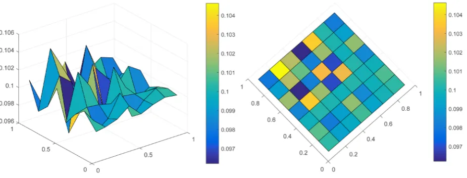
In the last section, we give a numerical example which illustrates the feasibility of the above method. The approximation solutions and mean solutions of the equations are shown in Figures 1-4.

Example 1. Consider the following two-dimensional nonlinear stochastic Itô-Volterra integral equation (one-dimensional case can reference to Example 1 in [17]).

(

)

(

)

(

)

(

)

(

)

( ) ( )

2 1

2

1 2 _{0 0} 1 2 1 2 1 2

2

1 2 1 2

0 0

1 1

, , 1 , d d

10 30

1 ₁ _, _d _d _.

30

t t

x t t x s s x s s s s

x s s B s B s

 

= −_ _ −

 

+ −

∫ ∫

The front view and the top view of the approximation solutions of the Exam-ple 1 for m = 8 are given in Figure 1.

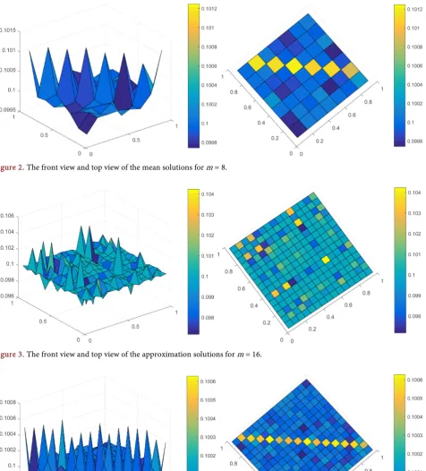
The front view and the top view of the mean solutions of the Example 1 for m

= 8 are given in Figure 2.

The front view and the top view of the approximation solutions of the Exam-ple 1 for m = 16 are given in Figure 3.

The front view and the top view of the mean solutions of the Example 1 for m

= 16 are given in Figure 4.

From these figures, we find the general trends of the solutions are similar for different m, and the absolute error of mean solution is very small. This method is efficient and the accuracy is credible.

8. Conclusion

[image:11.595.67.539.530.710.2]

For some stochastic Volterra integral equations, exact solutions cannot be ex-pressed. But, the numerical solution can be conveniently obtained based on dif-ferent stochastic numerical methods. As the complexity of the system, we use

(12)

[image:12.595.64.541.69.596.2]

Figure 2. The front view and top view of the mean solutions for m = 8.

[image:12.595.62.538.483.661.2]

Figure 3. The front view and top view of the approximation solutions for m = 16.

Figure 4. The front view and top view of the mean solutions for m = 16.

(13)

future, we will try to extend it to n-dimensional space and solve more problems.

Acknowledgements

We thank the Editors and the Reviewers for their helps and comments. This ar-ticle is funded by NSF Grants 11471105 of China, NSF Grants 2016CFB526 of Hubei Province, Innovation Team of the Educational Department of Hubei Province T201412, and Innovation Items of Hubei Normal University 2018032 and 2018105. These supports are greatly appreciated.

Conflicts of Interest

The authors declare no conflicts of interest regarding the publication of this pa-per.

References

[1] Hanson, R. and Phillips, J. (1978) Numerical Solution of Two-Dimensional Integral Equations Using Linear Elements. SIAM Journal on Numerical Analysis, 15, 113-121. https://doi.org/10.1137/0715007

[2] Babolian, E., Maleknejad, K. and Roodaki, M. (2010) Two-Dimensional Triangular Functions and Their Applications to Nonlinear 2D Volterra Fredholm Integral Eq-uations. Computers & Mathematics with Applications, 60, 1711-1722.

https://doi.org/10.1016/j.camwa.2010.07.002

[3] Fallahpour, M., Khodabin, M. and Maleknejad, K. (2015) Approximation Solution of Two-Dimensional Linear Stochastic Volterra Integral Equations by Applying the Haar Wavelets. International Journal of Mathematical Modelling and Computations (IJM2C), 5, 361-372.

[4] Jiang, Z.H. and Schaufelberger, W. (1992) Block Pulse Functions and Their Appli-cations in Control Systems. Spriger-Verlag, Berlin.

[5] Mirzaee, F. and Hadadiyan, E. (2014) Using Modified Two-Dimensional Block-Pulse Functions for the Numerical Solution of Nonlinear Two-Dimensional Volterra Integral Equations. Journal of Hyperstructures, 3, 68-80.

[6] Nemati, S., Lima, P.M. and Ordokhani, Y. (2013) Numerical Solution of a Class of Two-Dimensional Nonlinear Volterra Integral Equations Using Legendre Polyno-mials. Journal of Computational and Applied Mathematics, 242, 53-69.

https://doi.org/10.1016/j.cam.2012.10.021

[7] Fallahpour, M., Khodabin, M. and Maleknejad, K. (2016) Approximation Solution of Two-Dimensional Linear Stochastic Volterra-Fredholm Integral Equation via Two-Dimensional Block-Pulse Functions. International Journal of Industrial Ma-thematics, 8, Article ID: IJIM-00774.

[8] Maleknejad, K., Sohrabi, S. and Baranji, B. (2010) Application of 2D-BPFs to Non-linear Integral Equations. Communications in Nonlinear Science and Numerical Simulation, 15, 527-535. https://doi.org/10.1016/j.cnsns.2009.04.011

[9] Maleknejad, K. and Jafaribehbahani, Z. (2012) Applications of Two-Dimensional Triangular Functions for Solving Nonlinear Class of Mixed Volterra-Fredholm Integral Equations. Mathematical and Computer Modelling, 55, 1833-1844. https://doi.org/10.1016/j.mcm.2011.11.041

(14)

Journal of the Association of Arab Universities for Basic and Applied Sciences, 12, 65-73. https://doi.org/10.1016/j.jaubas.2012.05.001

[11] Aleknejad, K., Khodabin, M. and Shekarabi, F.H. (2014) Modified Block Pulse Functions for Numerical Solution of Stochastic Volterra Integral Equations. Journal of Applied Mathematics, 2014, Article ID: 469308.

[12] Maleknejad, K., Khodabin, M. and Rostami, M. (2012) Numerical Solution of Sto-chastic Volterra Integral Equation by a StoSto-chastic Operational Matrix Based on Block Pulse Function. Mathematical and Computer Modelling, 55, 791-800. https://doi.org/10.1016/j.mcm.2011.08.053

[13] Langville, A.N. and Stewart, W.J. (2004) The Kronecker product and Stochastic Automata Networks. Journal of Computational and Applied Mathematics, 167, 429-447. https://doi.org/10.1016/j.cam.2003.10.010

[14] Moler, C.B. (2006) Numerical Computing with MATLAB. China Machine Press, Beijing.

[15] Ezzati, R., Khodabin, M. and Sadati, Z. (2014) Numerical Implementation of Sto-chastic Operational Matrix Driven by a Fractional Brownian Motion for Solving a Stochastic Differential Equation. Abstract and Applied Analysis, 2014, Article ID: 523163.

[16] Maleknejad, K., Khodabin, M. and Rostami, M. (2012) A Numerical Method for Solving m-Dimensional Stochastic Itô-Volterra Integral Equations by Stochastic Operational Matrix. Computers & Mathematics with Applications, 63, 133-143. https://doi.org/10.1016/j.camwa.2011.10.079

[17] Mirzaee, F. and Samadyar, N. (2018) Numerical Solution of Nonlinear Stochastic Itô-Volterra Integral Equations Driven by Fractional Brownian Motion. Mathemat-ical Methods in the Applied Sciences, 14, 1410-1423.