Air quality index, ventilation coefficient and pollution potential studies over Bareilly city, Uttar Pradesh

AIR QUALITY INDEX, VENTILATION COEFFICIENT AND POLLUTION POTENTIAL STUDIES OVER

BAREILLY CITY, UTTAR PRADESH

1

_{Karuna, M. S.,}

_{Upadhyay, O. P.,}

1

_{IFTM University, Bareilly, Mooradabad,}

2

_{Department of Mechanical Engineering, Faculty of Engineering and Technology, M. J. P. Rohilkhand University,}

_{Department of Botany, B}

4

_{Department of Environmental Engineering, Sri Jayachamarajendra College of Engine}

ARTICLE INFO ABSTRACT

Ambient air quality monitoring (AAQM) along with assimilative capacity and Air Quality Index (AQI) studies were carried out at Indian Veterinary Research Institute (I.V.R.I), Izatnagar and Petrol Pump, Civil lines, Bareilly, India over a period of 5 year

and relative humidity was varied from 35°C to 45°C (March to May) and 96 % to 97 % (December) during 2013 to 2017. Maximum wind speeds were varying from 4 to 8 m s

to September and

directions over the study area. Maximum ventilation coefficient (VC) values were ranging from 9000 m2s-1 to 12000 m

ranging

negative assimilative potential of 190 to 230 μg m

and SPM, which were exceeding the NAAQS of 100 and 300 μg m

concentrations were found to be within 90 % of guideline values and assimilative potentials were ranging from 40

winter season and 300 found to be ranging from 300

Copyright © 2017, Karuna et al. This is an open access distribution, and reproduction in any medium, provided

INTRODUCTION

Due to the rapid urbanization and industrialization, air pollution has become a major environmental problem in both developed and developing countries (Chaurasia

Rapidly growth of motor vehicleswith time has resulted in traffic congestion, air pollution and noise problem

al., 2016). About 60 % of air pollution is contributed from automobile exhaust emission in Indian cities. Further, vehicular emission contains more than 450 different organic chemical compounds (Chaurasia et al., 2013).

sector is associated with the emission for about 50% of nitrogen oxide (NOx) and 90% of the carbon monoxide (CO) (Nagurney, 2000). In view of the above air pollution is often linked to substantial burdens of ill-health in developed and

*Corresponding author: Shobhan Majumder,

4_{Department of Environmental Engineering, Sri Jayachamarajendra College of}

Engineering, Mysuru, Karnataka, India.

ISSN: 0975-833X

Vol.

Article History:

Received 26th _{September, 2017}

Received in revised form 23rd _{October, 2017}

Accepted 18th _{November, 2017}

Published online 31st _{December, 2017}

Citation: Karuna, M. S., Upadhyay, O. P., Dinesh Kumar Saxena, Mahadeva Swamy, M. and Shobhan Majumder,

coefficient and pollution potential studies over Bareilly city, Uttar Pradesh”

Key words:

Ambient air quality, Assimilative Capacity, Ventilation Coefficient, Pollution Potential, Air Quality Index.

RESEARCH ARTICLE

AIR QUALITY INDEX, VENTILATION COEFFICIENT AND POLLUTION POTENTIAL STUDIES OVER

BAREILLY CITY, UTTAR PRADESH

Upadhyay, O. P.,

_{Dinesh Kumar Saxena,}

_{Mahadeva Swamy,}

and *

_{Shobhan Majumder}

IFTM University, Bareilly, Mooradabad, Uttar Pradesh, India

Department of Mechanical Engineering, Faculty of Engineering and Technology, M. J. P. Rohilkhand University,

Bareilly, Uttar Pradesh, India

Department of Botany, Bareilly College, Bareilly, Uttar Pradesh, India

Department of Environmental Engineering, Sri Jayachamarajendra College of Engine

Karnataka, India

ABSTRACT

Ambient air quality monitoring (AAQM) along with assimilative capacity and Air Quality Index (AQI) studies were carried out at Indian Veterinary Research Institute (I.V.R.I), Izatnagar and Petrol Pump, Civil lines, Bareilly, India over a period of 5 years from 2013 to 2017. Maximum temperature and relative humidity was varied from 35°C to 45°C (March to May) and 96 % to 97 % (December) during 2013 to 2017. Maximum wind speeds were varying from 4 to 8 m s

September and predominant wind was blowing from W and E followed by NW and WNW directions over the study area. Maximum ventilation coefficient (VC) values were ranging from 9000 to 12000 m2 s-1(from 13:00 h to 16:00 h) and for minimum wind speeds, VC values were ranging from 3000 m2 s-1to 4500 m2 s-1(from 12:00 h to 16:00 h) throughout the year. A maximum negative assimilative potential of 190 to 230 μg m-3 _{and 150 to 130 μg m}

and SPM, which were exceeding the NAAQS of 100 and 300 μg m

concentrations were found to be within 90 % of guideline values and assimilative potentials were ranging from 40 – 60 μg m-3at both the locations. AQI was found to be ranging from 350

winter season and 300 – 360 during summer and monsoon seasons. The annual average AQI was found to be ranging from 300 – 400, varying from ‘very poor’ to ‘sever’ AQI.

access article distributed under the Creative Commons Attribution License, the original work is properly cited.

and industrialization, air pollution has become a major environmental problem in both developed and developing countries (Chaurasia et al., 2013). Rapidly growth of motor vehicleswith time has resulted in traffic congestion, air pollution and noise problems (Mishra et ., 2016). About 60 % of air pollution is contributed from automobile exhaust emission in Indian cities. Further, vehicular emission contains more than 450 different organic ., 2013). Transportation s associated with the emission for about 50% of nitrogen oxide (NOx) and 90% of the carbon monoxide (CO) In view of the above air pollution is often

health in developed and

Department of Environmental Engineering, Sri Jayachamarajendra College of

developing countries, especially in India (Gorai Bruce et al., 2000; Smith et al

contains CO, hydrocarbons (HC), NOx, lead (Pb), dust (PM), carbon particles, sulphur dioxide (SO

pollutants react in presence of sunlight to produce secondary pollutants such as, O3, NO3, SO

pose harmful effect (acute and chronic diseases) on human health (Afroz et al., 2003; Kampa and Castanas, 2008) such as cardiovascular and respiratory disease, Neurological impairments, increased risk of preterm birth and even mortality and morbidity (Dohare and Panday, 2014). Further, many researchers have reported that outdoor air pollution negatively affects the productivity of indoor environment as well as workers (Wargocki et al., 2000;

et al., 2015). Dispersion of air pollutants is mainly dependent on meteorological factors.The two important meteorological factors which contributes the dispersion of pollutants include: mixing layer height (MLH) and wind speed (Emeis

International Journal of Current Research

Vol. 9, Issue, 12, pp.63243-63255, December, 2017

Karuna, M. S., Upadhyay, O. P., Dinesh Kumar Saxena, Mahadeva Swamy, M. and Shobhan Majumder,

coefficient and pollution potential studies over Bareilly city, Uttar Pradesh”, International Journal of Current Research, 9, (12),

Available online at http://www.journalcra.com

z

AIR QUALITY INDEX, VENTILATION COEFFICIENT AND POLLUTION POTENTIAL STUDIES OVER

Mahadeva Swamy, M.

Uttar Pradesh, India

Department of Mechanical Engineering, Faculty of Engineering and Technology, M. J. P. Rohilkhand University,

Bareilly, Uttar Pradesh, India

Department of Environmental Engineering, Sri Jayachamarajendra College of Engineering, Mysuru,

Ambient air quality monitoring (AAQM) along with assimilative capacity and Air Quality Index (AQI) studies were carried out at Indian Veterinary Research Institute (I.V.R.I), Izatnagar and Petrol s from 2013 to 2017. Maximum temperature and relative humidity was varied from 35°C to 45°C (March to May) and 96 % to 97 % (December) during 2013 to 2017. Maximum wind speeds were varying from 4 to 8 m s-1 during the month of June nant wind was blowing from W and E followed by NW and WNW directions over the study area. Maximum ventilation coefficient (VC) values were ranging from 9000 (from 13:00 h to 16:00 h) and for minimum wind speeds, VC values were (from 12:00 h to 16:00 h) throughout the year. A maximum and 150 to 130 μg m-3_{was observed for RSPM} and SPM, which were exceeding the NAAQS of 100 and 300 μg m-3, respectively. SO2 and NOx concentrations were found to be within 90 % of guideline values and assimilative potentials were at both the locations. AQI was found to be ranging from 350 – 400 during nd monsoon seasons. The annual average AQI was 400, varying from ‘very poor’ to ‘sever’ AQI.

License, which permits unrestricted use,

developing countries, especially in India (Gorai et al., 2014; et al., 2000).Vehicular exhaust contains CO, hydrocarbons (HC), NOx, lead (Pb), dust (PM), carbon particles, sulphur dioxide (SO2), etc. Some of these pollutants react in presence of sunlight to produce secondary , SO2, PAN.These pollutants may pose harmful effect (acute and chronic diseases) on human ., 2003; Kampa and Castanas, 2008) such as cardiovascular and respiratory disease, Neurological impairments, increased risk of preterm birth and even mortality morbidity (Dohare and Panday, 2014). Further, many researchers have reported that outdoor air pollution negatively affects the productivity of indoor environment as well as ., 2000; Kosonen, and Tan, 2004; Choi sion of air pollutants is mainly dependent on meteorological factors.The two important meteorological factors which contributes the dispersion of pollutants include: mixing layer height (MLH) and wind speed (Emeis et al.,

INTERNATIONAL JOURNAL OF CURRENT RESEARCH

2008; Schafer et al., 2006; Ghiaus et al., 2006; Chan 2012). The MLH indicates the vertical dilution of air pollutants, and wind speed represents the horizontal ventilation, which helps to reduce ground level pollutant concentration. Further, ventilation coefficient (VC) is a product of mean mixing depth (MMD) and average wind speed, which gives an indication of the air quality in terms of the ability of the atmosphere to disperse the pollutants over a region (Motesaddi et al., 2008; Goyal et al

Raj, 2013). Many researchers have conducted studies on assimilative capacity based on ventilation coefficient and pollution potential (Maria et al., 2000; Rigby

Goyal et al., 2002; Chan et al., 2012; Sujatha and Raj, 2013; Abiye et al., 2016; Alappattu

et al. (2012) have stated that VC was significantly variable and maximum was found to be during day-time, while VC was relatively invariable and minimum during night

indicates that, the reasonable time to emit maximum

air pollutant is during daytime particularly at noon due to the occurrence of highest VC. However, Iyer and Raj (2013) have reported in Delhi city VC decreased at the rate of 49 and 32 m s-1year-1 in the months of December and February, respectively, during last 30-year period. However, in Mumbai, average decrease in VC in winter seasons was 15 m

1

and for Kolkata it was 14 and 17 m2 s-1 year

February, respectively. Kumar et al. (2015) have developed a conjunction model of Wavelet-Neuro-fuzzy model for accurate prediction of the VC over the capital region of Delhi, India. The result of the predicted values obtained from the model was found to be satisfactory.It was also quoted that, Wavelet Neuro-fuzzy model has mean absolute error of 0.0058 in testing series and 0.0312 in training series. Abiye

have reported characteristic values of the atmospheric ventilation coefficients varied from month to month and from daytime (08:00 to 19:00, GMT+1) to night

07:00, GMT+1) with daily maximum values occurring in the late afternoon between (13:00 to 17: 00, GMT+1) in Nigeria. The maximum VC values obtained were 1216 m

m2 s-1, 1760 m2 s-1and 1038 m2 s-1, 1225 m2

and 1334 and 436 m2 s-1from September to December, 2012 and 2013, respectively. On the other hand, Air Pollution Index (API) Reporting System is an important tool for risk communication, which informs public about the ambient air pollution level and the potential health risk associated with the pollution level (Taieb and Brahim, 2013).

Earlier many researchers (Sharma et al., 2003a, 2003b; Murena, 2004; Nagendra et al., 2007; Wen et al

al., 2010; Choi et al., 2015; Bhuyan et al

calculated AQI developed by the USEPA to analyse the daily air quality.Wang and Lu (2006) have developed revised AQI for Hong Kong city and varying trends of AQI and analysed during 1999 and 2003. It was found that, daily mean AQI during the seasonal period can be regarded as stationary time series (Wang and Lu, 2006). However, Prakash

have reported during winter season AQI was found to be ‘Moderate’ (141) at Hebbal industrial area, due to high pollution load of PM10 (> 100 μg m-3). However, during summer and monsoon season AQI was found to be ‘Satisfactory’ and ‘good’ due to high wind speeds and occurrence of precipitation. Sonibare et al. (2010) have stated that, the AQI for measured CO concentrations in Niger Delta area, Nigeria, ranged between 1 and 44, which indicates a ‘good’ AQI category and over 97 % of the measured NO concentrations were below 0.60 ppm which also implies a

., 2006; Chan et al., 2012). The MLH indicates the vertical dilution of air pollutants, and wind speed represents the horizontal ventilation, which helps to reduce ground level pollutant concentration. Further, ventilation coefficient (VC) is a ct of mean mixing depth (MMD) and average wind speed, which gives an indication of the air quality in terms of the ability of the atmosphere to disperse the pollutants over a et al., 2007; Iyer and earchers have conducted studies on assimilative capacity based on ventilation coefficient and ., 2000; Rigby et al., 2006; ., 2012; Sujatha et al., 2016; Iyer Alappattu et al., 2009).Chan . (2012) have stated that VC was significantly variable and time, while VC was relatively invariable and minimum during night-time. It indicates that, the reasonable time to emit maximum amount of air pollutant is during daytime particularly at noon due to the However, Iyer and Raj (2013) have reported in Delhi city VC decreased at the rate of 49 and 32 m2

in the months of December and February, year period. However, in Mumbai, average decrease in VC in winter seasons was 15 m2 s-1 year

-year-1in December and . (2015) have developed a fuzzy model for accurate prediction of the VC over the capital region of Delhi, India. The result of the predicted values obtained from the model was found to be satisfactory.It was also quoted that,

Wavelet-lute error of 0.0058 in testing series and 0.0312 in training series. Abiye et al. (2016) have reported characteristic values of the atmospheric ventilation coefficients varied from month to month and from daytime (08:00 to 19:00, GMT+1) to night-time (20:00 to 07:00, GMT+1) with daily maximum values occurring in the late afternoon between (13:00 to 17: 00, GMT+1) in Nigeria. The maximum VC values obtained were 1216 m2 s-1and 1156 s-1and 691 m2 s-1, from September to December, 2012 On the other hand, Air Pollution Index (API) Reporting System is an important tool for risk communication, which informs public about the ambient air h risk associated with the

et al., 2003a, 2003b; et al., 2009; Eder et et al., 2010) have QI developed by the USEPA to analyse the daily air quality.Wang and Lu (2006) have developed revised AQI for Hong Kong city and varying trends of AQI and analysed during 1999 and 2003. It was found that, daily mean AQI arded as stationary time series (Wang and Lu, 2006). However, Prakash et al. (2017) have reported during winter season AQI was found to be ‘Moderate’ (141) at Hebbal industrial area, due to high ). However, during r and monsoon season AQI was found to be ‘Satisfactory’ and ‘good’ due to high wind speeds and . (2010) have stated that, the AQI for measured CO concentrations in Niger Delta 44, which indicates a ‘good’ AQI category and over 97 % of the measured NO2 concentrations were below 0.60 ppm which also implies a

good category of AQI with no health effects. The number of vehicular population is increasing with time in Bareilly city, which results in a poor air quality near to the road canyon. Hence, an attempt was made to represent the overall meteorological factors and carrying capacity of the atmosphere in terms of ventilation coefficient and pollution potential over Bareilly city, Uttar Pradesh, India.

Study area

Bareilly city is in North Indian state of Uttar Pradesh, India. It is the capital of Bareilly division and the geographical region of Rohilkhand.In the present study, ambient air quality monitoring (AAQM) have been conduct

Research Institute (I.V.R.I), Izatnagar (Location 1) and Petrol Pump, Civil lines, (Location 2) Bareilly, India (Fig. 1 a

Fig. 1(a). Google Earth view of Location 1 with Ambient Air Quality Monitoring Station (AAQMS) and se

to the Indian Veterinary Researc

Fig. 1(b). Google Earth view of Location 2 with Ambient Air Quality Monitoring Station (AAQMS) and selected highway near

to the Petrol Pump, Civil lines, Bareilly

Location 1 (IVRI institute) is located at the Northern part of Bareilly district, Izatnagar, Uttar Pradesh. On the other hand, good category of AQI with no health effects. The number of vehicular population is increasing with time in Bareilly city, ich results in a poor air quality near to the road canyon. Hence, an attempt was made to represent the overall meteorological factors and carrying capacity of the atmosphere in terms of ventilation coefficient and pollution potential over

tar Pradesh, India.

Bareilly city is in North Indian state of Uttar Pradesh, India. It is the capital of Bareilly division and the geographical region of Rohilkhand.In the present study, ambient air quality monitoring (AAQM) have been conducted at Indian Veterinary Research Institute (I.V.R.I), Izatnagar (Location 1) and Petrol Pump, Civil lines, (Location 2) Bareilly, India (Fig. 1 a-b).

Fig. 1(a). Google Earth view of Location 1 with Ambient Air Quality Monitoring Station (AAQMS) and selected highway near to the Indian Veterinary Research Institute (I.V.R.I) Izatnagar

Fig. 1(b). Google Earth view of Location 2 with Ambient Air Quality Monitoring Station (AAQMS) and selected highway near

rol Pump, Civil lines, Bareilly

Petrol Pump is located Southern part of Bareilly district, Civil lines, Uttar Pradesh, India. The elevation of the study area varies from 162 m to 176 m. Minimum elevation observed in the centre of the Location 1 (IVRI institute) and North West part of the Location 2 (Petrol Pump). However, Location 1 (IVRI institute) comprises of institutional area, residential area and commercial area. The second location (Petrol Pump, Civil lines) comprises of commercial area, traffic intersection and market area. Near to the AAQM stations there is no nearby industries, and thereby major sources of pollution was mainly due to line sources (vehicular emission).

MATERIALS AND METHODS

Meteorological Data Collection

Various meteorological parameters that influence the dispersion of air pollutants include: wind speed and its direction, temperature, precipitation, relative humidity, mean mixing depth (MMD), atmospheric pressure, cloud cover, heating effects and nature of terrain. Hourly meteorological data was obtained from the website www.wunderground.com which was used for plotting the monthly variation of meteorological factors from 2013 to 2017 over Bareilly city.

Assimilative Capacity

Assimilative capacity or Carrying Capacity refers to the ability of the environment of a particular region to carry the pollutants without adverse effects on the environment or on users of its resources (Manju et al., 2002). The assimilative capacity of the atmosphere can be determined using two approaches. First approach isbased on ventilation coefficient (VC), which can be calculated by meteorological parameters and the second approach is based on pollution potential, which is due to the presence of air pollutants in the environment. The pollution potential indicates the capacity of the atmosphere to dilute the pollutants and the resulting effects on air quality.

Assimilative capacity based on ventilation coefficient

Ventilation coefficient is the product of mixing depth and average wind speed and can be calculated by using Eqn. 1. The higher the coefficient, the more efficiently the atmosphere can able to disperse the pollutants and better is the air quality. On the other hand, low ventilation coefficients lead to poor dispersion of pollutants causing stagnation and poor air quality leading to possible pollution related hazards (Iyer and Raj, 2013).

Ventilation coefficient (m2s-1) = Wind speed (m s-1)xMMD (m) (1)

The US National Meteorological Centre and Atmospheric Environment Services, Canada, has classified that, high pollution potential or low assimilative capacity occurs during afternoon, when ventilation coefficient is < 6000 m2s-1 and mean wind speed does not exceed 4 m s-1 and during morning hours, when mixing height is < 500 m.

Assimilative capacity based on pollution potential

The second approach is based on the pollution potential in terms of pollutant concentrations measured during AAQM days. Assimilative capacity was determined by considering the

difference between the permissible and the existing pollutant concentration levels, for the study region, using Eqn. 2.

Available assimilation potential = Permissible standard – Pollutant concentration (2)

Air Quality Index (AQI)

Air Quality Index (AQI) is a tool introduced by Environmental Protection agency (EPA), USA to measure the levels of pollution due to major air pollutants. AQI focuses on health effects that may experience within a few hours or days after breathing the polluted air. EPA calculates the AQI for five major air pollutants regulated by the Clean Air Act. These include: ground-level ozone, particle pollution (as particulate matter), carbon monoxide, sulphur dioxide and nitrogen dioxide. In the present study AQI was calculated as specified by Sharma et al. (2001, 2003b) (Eqn. 3) for the study period, based on the ambient air quality monitored data obtained from 2013 to 2017. The AQI focuses on health effects that may experience within a few hours or days after breathing polluted air.





PLO PHI

LO HI

P

C

B

I

B

B

I

I

I

_





















*

(3)

Where, IP is AQI for pollutant “P”, CP is the actual ambient concentration of pollutant “P”, BPHI is the upper end breakpoint concentration that is greater than or equal to CP, BPLO is the lower end breakpoint concentration that is less than or equal to CP, ILO is the sub index or AQI value corresponding to BPLO, IHI is the sub index or AQI value corresponding to BPHI.

RESULTS AND DISCUSSION

Meteorological data

Monthly, seasonal and annual variation of temperature, relative humidity and precipitation

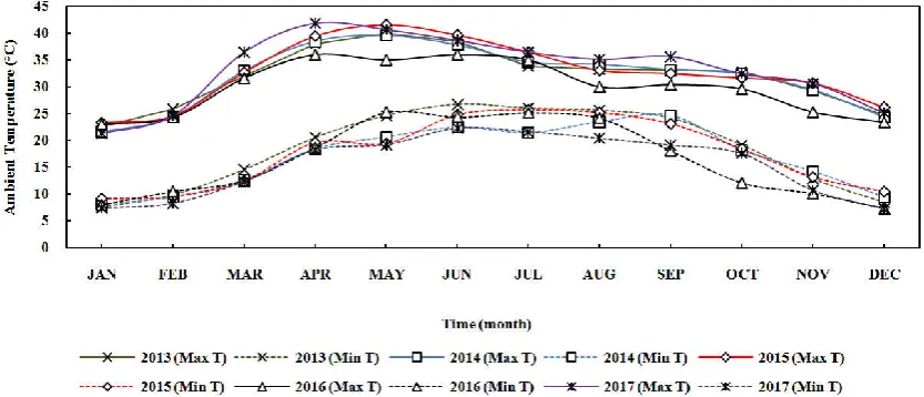
The data of maximum and minimum temperature and relative humidity of the atmosphere were collected from IMD Lucknowover a period of 5 years from 2013 to 2017 considering winter, summer and monsoon seasons from January to December over the study area. Plots of ambient temperature and humidity against time were made shown in Figures 2 and 3. It was observed that, maximum temperatures were varied from 35°C to 45°C, in the month of March to May, of 2013 to 2015 and 2017. However, minimum temperatures were varied from 8°C to 10°Cduring December to February of 2013 to 2017. The maximum temperature of ~ 45°C was observed in the month of April, 2017 and a minimum temperature of 7°C was observed in the month of January, 2017. It was noticed that, temperature was minimum at 03:00 h to 07:00 h and it gradually increased and reached the peak at 13:00 to 16:00 h and then started decreasing during winter, summer and monsoon seasons. Further, a maximum temperature of 40°C was observed in the month of May, 2013 and 2014, and a minimum temperature of ~ 7°C was noticed in the month of January, 2013 and 2014. As temperature increases wind speed also increases which leads to an unstable atmospheric condition, which is more favourable for rapid dispersion of pollutants. Relative humidity (RH) is the ratio of the partial pressure of water vapour to the equilibrium vapour

pressure of water at a given temperature. Relative humidity depends on temperature and the pressure of the system of interest. Figure 3, shows a plot of relative humidity versus time for month wise annual variation of maximum and minimum relative humidity (RH). A minimum humidity of 25 % was noticed during the month of January, 2017. Low relative humidity and low clouds represents low pollution levels. However, maximum humidity of 96 % to 97 % was observed in Month of December, 2016 and 2017, respectively, which represents high pollution levels. It was also found that, maximum RH were varied from 80 – 97 % throughout the year, depending upon the atmospheric conditions such as, temperature and precipitation.

It was also observed that, RH was minimum at 02:00 to 07:00 h and it gradually increased and reached peak value at 14:00 to 17:00 h and then started decreasing. Figure 4 shows a plot of precipitation versus time over a period of 5 years from 2013 to 2017. It was found that, maximum precipitation occurs in the month of July to October and minimum precipitation occurred in rest of the months. It was also found that, a maximum precipitation of 50 mm, 38 mm and 28 mm recorded in the month of July to August, 2013, 2014 and 2015, respectively. From the precipitation data, it can be ascertained that, during the month of July to September ambient pollutant concentration found to be minimum due to the occurrence of maximum precipitation.

Fig. 2. Monthly variation of maximum and minimum ambient temperature over Bareilly city from 2013 to 2017

Fig. 3. Monthly variation of maximum and minimum relative humidity over Bareilly city from 2013 to 2017

Seasonal variation of maximum mixing depth (MMD)

MMD is the amount of air available to dilute pollutants is related to the wind speed and to the extent to which emissions can rise into the atmosphere. Mixing depth is used to quantify the vertical mixing of pollutants in the atmosphere. A plot of minimum and maximum MMD during winter, summer and post-monsoon season against time is made shown in Figure 5.

It was found that, the mean mixing depth varies seasonally as well as hourly. From the plot it was observed that, MMD was minimum during morning hours, it gradually increased and reached the peak at 14:00 to 16:00 h and there onwards it started decreasing in all the seasons. The variation of MMD was mainly due to ambient temperature and wind speeds. It is observed that, mixing depth was found to be maximum during

Fig. 5. Plot of minimum and maximum MMD during winter, summer and post-monsoon season over Bareilly city

Fig. 6. Monthly variation of maximum and minimum wind speeds over Bareilly city from 2013 to 2017

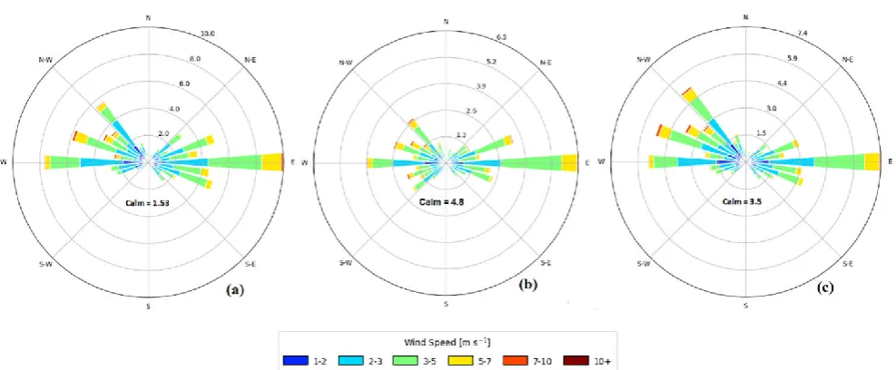
Fig. 7. Windrose plots for (a) 2013, (b) 2017 and (c) 2013 to 2017 over Bareilly city, Uttar Pradesh, India

mmer season, which may be due to the high ambient temperature and relatively high wind velocities during summer season (March to May) when compared to during winter season. It is also observed that, mixing heights were lowest during post-monsoon season; this may be due to lower inversion layer and cloud cover. The very low values of mixing height during late nights and early morning hours could be due to the occurrence of ground-based inversions which reducesdegree of dispersion (Padmanabhamurty and Mandal, 1979).

Monthly, seasonal and annual variation of wind speeds

The magnitude and directionof wind arethe major meteorological factors which govern the dispersion of air

pollutants over a study area. A plot of wind velocity versus time for season wise monthly varied wind speeds has been made shown in Figure 6. It was found that, maximum wind speeds were varying from 4 to 8 m s-1 during June to September, 2013 to 2017. However, a minimum wind speed of ~ 0 m s-1 was observed during 2015. It can be seen that, a maximum wind velocity of 8 m s-1 was recorded in the month of August, 2014 and 2017, which implies a favourable atmospheric condition for the dispersion of pollutants.

However, a fluctuation of wind speeds was noticed throughout the year due to variation in temperature and stability class. The average wind speeds were varying from 2.22 m s-1to 3.889 m s -1

during the study period.

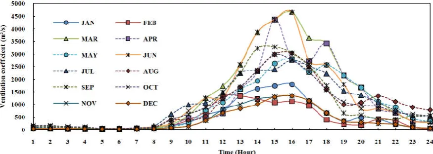
Fig. 8(a). Diurnal variation of maximum ventilation coefficients during January to December for maximum wind speeds and MMD

Fig. 8(b). Diurnal variation of maximum ventilation coefficients during January to December for minimum wind speeds and MMD

Wind rose plots

Wind rose plot is a graphical representation of frequency and distribution of wind over a period of time at a specific location. To create a wind rose, average wind velocity and its directions are logged at a site, at short intervals, over a period of time i.e., from 2013 to 2017. Annual variation of wind rose diagrams for the study period from 2013 to 2017 were plotted using WRPLOT and shown in Figure 7 (a, b and c). The annual wind rose plot during 2013 and 2017 showed similar wind directions with predominant wind directions from W and E followed by NW and WNW directions, which were blowing towards E, W, SE and ESE directions over the study area. The average wind velocity were ranging from 2 – 5 m s-1 with a calm period of 0.5 to 4.8 %.

Carrying Capacity of the Atmosphere

Assimilative capacity refers to the ability of the atmosphere to carry pollutants without adverse effects on the environment. The assimilation potential (assimilative capacity) of the atmosphere can be represented by two ways i.e., ventilation coefficient, which is a product of product of MMD and wind speeds and the second approach is dispersion potential of emission loads discharged into the region (Goyal and Rao, 2007). The details of the role of ventilation coefficient and pollution potential on the dispersion of air pollutants in the atmosphere have been discussed in the following sub-sections.

Carrying capacity based on ventilation coefficient (VC)

Ventilation Coefficient (VC) is directly proportional to the carrying capacity or assimilative potential of the atmosphere can be calculated using MMD and wind speeds from January to December over a period of 5 years i.e., from 2013 to 2017. Ventilation coefficient plays an important role on the dispersion of aerosols, and can be considered as one of the factors determining pollution potential over a region (Chan et al., 2012). Plots of maximum ventilation coefficients for maximum and minimum wind speed, MMD against time during January to December were made shown in Figures 8 (a, b). It was observed that, wind speeds, MMD and ventilation coefficient (VC) values were found to be less during late nights and early morning periods. During January, a maximum VC of 4500 m2s-1 (at 15:00 h) (Figure 8a) was observed with maximum wind speeds. A minimum VC of 1800 m2 s-1 (at 16:00 h) was noticed with minimum wind speeds and MMD. However, both the VCs were found to be less than the favourable VC for safe dispersion of 6000 m2 s-1. The reason for obtaining lower VC may be due to the stable atmospheric conditions during the month of January. Wind speeds were found to be ranging from 2 – 3 m s-1, which allows a calm atmospheric condition. Further, in the month of February, a maximum VC of 4600 m2 s-1 (at 15:00 h) was observed with maximum wind speeds. A minimum VC of 1400 m2 s-1 (at 12:00 h) was noticed with minimum wind speeds and MMD.

Fig. 9(b). Diurnal variation of maximum ventilation coefficients over Bareilly city during summer season from 2013 to 2017 for maximum and minimum wind speeds

Fig. 9(c). Diurnal variation of maximum ventilation coefficients over Bareilly city during monsoon season from 2013 to 2017 for maximum and minimum wind speeds

The reason for obtaining lower VC may be due to the stable atmospheric condition in the winter season. However, in the month of March, April and May a maximum VC of 10000 m2 s-1to 12000 m2 s-1 (at 17:00 h to 18:00 h) was observed with maximum wind speeds (Figure 8a). A minimum VC of 3000 m2 s-1to 4500 m2 s-1 (at 15:00 h to 16:00 h) was observed with minimum wind speeds and MMD. The maximum VCs were found to be more than the favourable VC for safe dispersion of 6000 m2 s-1, which implies a better mixing of pollutants occurred in the atmosphere. The reason for obtaining higher VC values during March and April may be due to the unstable atmospheric condition as the wind speeds were varying from 6 – 9 m s-1. The variation of VC in all the months were found to be similar except the variation of the VC values. Maximum VC values were ranging from 9000 m2 s-1to 12000 m2 s-1(from 13:00 h to 16:00 h) and minimum VC values were ranging from 3000 m2 s-1to 4500 m2 s-1(from 12:00 h to 16:00 h) during the month of June to December. Manju et al. (2002) have reported that, maximum VC was recorded as 7900 m2 s-1in summer followed by pre-monsoon and monsoon with 4340 m2 s-1and 4060 m2 s-1, respectively, in Manali, India. Krishna et al. (2004) have reported a maximum VC of 13,924 m2 s-1was noticed during season when compared to 9781 m2 s-1during summer, at Visakhapatnam, India.

Further, plots of diurnal variation of minimum and maximum ventilation coefficient versus time over Bareilly city during winter, summer and monsoon seasons from 2013 to 2017 were made shown in Figures 9 (a, b, c). Hourly computed VC showed a similar diurnal trend in all the three seasons. Various researchers have calculated VC to understand the assimilative potential of the atmosphere (Krishna et al., 2004; Goyal et al., 2005; Goyal and Rao, 2007, Thepanondh and Jitbantoung, 2014; Thawonkaew et al., 2016). With an increase in solar insolation, as the day advances VC also increases reaching a maximum value during afternoon hours. Further, in the evening hours when incoming solar radiation ceases the VC gradually decreases (Viswanadham and Kumar, 1989). The ventilation coefficient values were very low (less than 1000 m2 s-1) during the morning (01:00 – 09:00 h) and evening/night hours (20:00 – 24:00 h) indicating high pollution potential or low assimilative capacity during these periods (Figure 9). Duringwinter, maximum VC was found to be ~ 2200 m2 s-1 (at 16:00 h) during 2017, followed by 2000 m2 s-1 (at 17:00 h during 2013) and 1400 m2 s-1(at 12:00 h during 2014) at minimum wind speeds and MMD (Figure 9a). High or low wind speeds and variation in mixing heights were the causes for varied ventilation coefficients. The minimum VCs were found to be < 6000 m2 s-1, which indicate high pollution potential. Further, during the winter season, maximum VC was found to be ~ 6000 m2 s-1 (at 16:00 h) during 2016 and 2017, followed by 4500 m2 s-1 (at 15:00 h during 2013 and 2014) at maximum wind speeds and MMD (Figure 9a). The maximum VCs were found to be < 6000 m2 s-1, which indicates high pollution potential or low assimilative capacity during these periods. During summer season ventilation coefficient values were found to be less than 1000 m2 s-1during morning early morning and evening/night hours. During summer, maximum VC was found to be maximum of ~ 5000 m2 s-1 (at 14:00 h to 17:00 h) at minimum wind speeds during 2014 to 2017 (Figure 9-b), which was found to be < 6000 m2 s-1, indicating high pollution potential. Further, during summerseason, maximum VC was found to be ~ 15000 m2 s-1(at 16:00 h) during 2017, followed by 13000 m2 s-1 (at 16:00 h during 2016), 11000 m2 s-1 (at 16:00 h during 2015). The maximum VCs were found to

be > 6000 m2 s-1 indicating that low pollution potential or high assimilative capacity during these periods. The ventilation coefficient was found to be highest in summer season than winter. Infect, during monsoon season maximum VC was found to be ~ 9000 m2 s-1(at 15:00 h) during 2013, 2014 and 2017, followed by 8000 m2 s-1(at 16:00 h during 2016) (Figure 9c). High or low wind speed and mixing height are responsible for the variability (Goyal and Rao, 2007). From the above it is observed that, pollution potential found to be high during winter as compared to summer and monsoon periods. Thus, it can be concluded that, the VC simply provides a broad indication of the dispersion potential in terms of low (< 2000 m2 s-1), medium (2000 – 6000 m2 s-1) or high (> 6000 m2 s-1) of the atmosphere. However, it does not give any idea about the amount of emission loads that can be assimilated in the given air-shed of the region (Goyal and Rao, 2007). Sujatha et al. (2016) have estimated ventilation coefficient (VC) in order to understand the dispersion of pollutants over the urban region of Hyderabad during 2009 – 2011. The result showed that, boundary layer height (BLH) was maximum in summer and minimum in monsoon period, whereas, the maximum VC was observed during summer and minimum in winter.

Effect of emission loads on carrying capacity of the atmosphere

Table 1. Assimilative capacity of the atmosphere in terms of pollution potential for RSPM from 2013 – 2017

Month NAAQS (μg/m³) 90% of guideline (μg/m³) IVRI institute (μg m

-3_{) Petrol Pump (μg m}-3₎

2013 2014 2015 2016 2017 2013 2014 2015 2016 2017

January 100 90 -158 -120 -185 -230 -170 -230 -235 -230 -230 -260

February 100 90 -190 -130 -135 -150 -160 -210 -185 -210 -210 -210

March 100 90 -140 -110 -135 68 -170 -210 -185 -160 -260 -260

April 100 90 -140 -100 -110 -110 -160 -210 -185 -160 -160 -210

May 100 90 -110 -100 -135 -130 -120 -190 -160 -210 -160 -210

June 100 90 -110 -135 -135 -130 -140 -210 -160 -185 -170 -140

July 100 90 -110 -120 -110 -110 -90 -160 -160 -170 -210 -110

August 100 90 -110 -120 -110 -110 -100 -185 -210 -170 -190 -130

September 100 90 -110 -110 -130 -110 -100 -190 -190 -190 -185 -160

October 100 90 -90 -110 -130 -90 -110 -170 -185 -170 -210 -210

November 100 90 -140 -160 -140 -100 -120 -210 -230 -210 -220 -410

December 100 90 -160 -160 -175 -130 -130 -210 -210 -220 -230 -260

Table 2. Assimilative capacity of the atmosphere in terms of pollution potential for SPM from 2013 – 2017

Month NAAQS (μg/m³) 90% of guideline (μg/m³) IVRI institute (μg m

-3

) Petrol Pump (μg m-3)

2013 2014 2015 2016 2017 2013 2014 2015 2016 2017

January 300 270 -100 -30 -55 -105 -70 -130 -130 -130 -130 -180

February 300 270 -150 -50 -50 -80 -40 -80 -80 -80 -80 -180

March 300 270 -100 -30 -30 -30 -50 -80 -55 -30 -60 -280

April 300 270 -80 -30 -30 -10 -50 -105 -50 -40 -105 -180

May 300 270 -80 -10 -30 -30 -55 -55 -30 20 -105 -130

June 300 270 -30 -50 -30 -30 -70 -130 -55 -55 -130 -80

July 300 270 -30 -50 -30 -30 -5 -55 -50 -50 -55 -80

August 300 270 -30 -30 -30 -30 -5 -80 -80 -60 -80 -80

September 300 270 -30 -30 -50 -30 0 -55 -70 -40 -105 -80

October 300 270 -30 -30 -30 -30 -10 -55 -80 -80 -110 -130

November 300 270 -130 -80 -40 0 -30 -80 -130 -105 -100 -480

December 300 270 -110 -80 -55 -80 -40 -80 -105 -130 -130 -180

Table 3. Assimilative capacity of the atmosphere in terms of pollution potential for SO2 from 2013 – 2017

Month NAAQS (μg/m³) 90% of guideline (μg/m³) IVRI institute (μg m

-3

) Petrol Pump (μg m-3)

2013 2014 2015 2016 2017 2013 2014 2015 2016 2017

January 80 72 61 62 61 62 61 60 59 60 58 57

February 80 72 62 60 59 60 60 58 57 60 58 58

March 80 72 60 60 60 61 61 54 58 59 59 60

April 80 72 62 59 61 60 60 58 60 57 58 56

May 80 72 59 60 61 60 61 57 59 57 57 56

June 80 72 62 59 59 58 60 55 57 56 58 57

July 80 72 59 62 61 61 62 59 60 60 61 54

August 80 72 65 60 61 59 61 58 59 59 60 58

September 80 72 60 60 61 61 61 58 60 58 57 52

October 80 72 62 61 60 60 60 58 58 59 59 57

November 80 72 60 58 59 60 60 55 57 60 56 56

December 80 72 60 63 60 60 59 59 58 59 59 57

Table 4. Assimilative capacity of the atmosphere in terms of pollution potential for NOx from 2013 – 2017

Month NAAQS (μg/m³) 90% of guideline (μg/m³) IVRI institute (μg m

-3

) Petrol Pump (μg m-3)

2013 2014 2015 2016 2017 2013 2014 2015 2016 2017

January 80 72 51 51 50 51 51 45 46 43 46 40

February 80 72 52 52 49 48 51 46 46 44 45 37

March 80 72 52 50 50 47 50 44 47 45 45 44

April 80 72 42 50 46 48 48 44 46 44 42 35

May 80 72 40 48 47 52 48 45 42 47 40 35

June 80 72 47 47 42 50 51 46 41 46 46 42

July 80 72 50 52 48 49 52 47 42 47 40 43

August 80 72 47 53 50 47 52 40 36 45 44 47

September 80 72 52 51 49 48 53 44 42 42 46 47

October 80 72 43 48 45 46 52 43 39 43 42 37

November 80 72 52 47 40 48 48 46 41 44 45 40

December 80 72 49 47 42 47 48 46 34 41 47 37

Table 5. Air Quality Index at IVRI institute and Petrol pump, Izatnagar during 2013

Month IVRI institute (Conc. in µg m

-3_{) Petrol Pump (Conc. in µg m}-3₎

RSPM SPM SO2 NOx AQI RSPM SPM SO2 NOx AQI

January 248 370 11 21 398 320 400 12 27 454

February 280 420 10 20 423 300 350 14 26 438

March 230 370 12 20 385 300 350 18 28 438

April 230 350 10 30 385 300 375 14 28 438

May 200 350 13 32 362 280 325 15 27 423

June 200 300 10 25 362 300 400 17 26 438

July 200 300 13 22 362 250 325 13 25 400

August 200 300 7 25 362 275 350 14 32 419

September 200 300 12 20 362 280 325 14 28 423

October 180 300 10 29 346 260 325 14 29 408

November 230 400 12 20 385 300 350 17 26 438

December 250 380 12 23 400 300 350 13 26 438

Hence, SO2 and NOx concentrations were found to be within 90 % of guideline values from January to December during 2013, indicated a positive assimilative potential at both the locations. However, SO2 concentration was found to be minimum when compared to NOx, thus a maximum assimilative potential was found for SO2. Assimilative potentials were ranging from 40 – 60 μg m-3at location 1 and 2, shows a significantly good carrying capacity of the atmosphere in terms of SO2 and NOx (Tables3 and 4).

Further, a negative assimilative potential was found during 2014 – 2017 for the pollutants RSPM and SPM (Tables 1 and 2), which may be due to vehicular exhaust and fugitive emissions and increased number of vehicles during the study period. However, pollution potential was found to be maximum during winter season (December to February) when compared to summer and monsoon seasons (March to September).

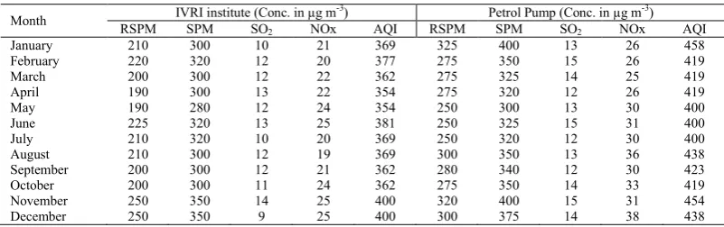
Table 6. Air Quality Index at IVRI institute and Petrol pump, Izatnagar during 2014

Month IVRI institute (Conc. in µg m

-3_{) Petrol Pump (Conc. in µg m}-3₎

RSPM SPM SO2 NOx AQI RSPM SPM SO2 NOx AQI

January 210 300 10 21 369 325 400 13 26 458

February 220 320 12 20 377 275 350 15 26 419

March 200 300 12 22 362 275 325 14 25 419

April 190 300 13 22 354 275 320 12 26 419

May 190 280 12 24 354 250 300 13 30 400

June 225 320 13 25 381 250 325 15 31 400

July 210 320 10 20 369 250 320 12 30 400

August 210 300 12 19 369 300 350 13 36 438

September 200 300 12 21 362 280 340 12 30 423

October 200 300 11 24 362 275 350 14 33 419

November 250 350 14 25 400 320 400 15 31 454

December 250 350 9 25 400 300 375 14 38 438

Table 7. Air Quality Index at IVRI institute and Petrol pump, Izatnagar during 2015

Month IVRI institute (Conc. in µg m

-3_{) Petrol Pump (Conc. in µg m}-3₎

RSPM SPM SO2 NOx AQI RSPM SPM SO2 NOx AQI

January 275 325 11 22 419 320 400 12 29 454

February 225 320 13 23 381 300 350 12 28 438

March 225 300 12 22 381 250 300 13 27 400

April 200 300 11 26 362 250 310 15 28 400

May 225 300 11 25 381 300 250 15 25 438

June 225 300 13 30 381 275 325 16 26 419

July 200 300 11 24 362 260 320 12 25 408

August 200 300 11 22 362 260 330 13 27 408

September 220 320 11 23 377 280 310 14 30 423

October 220 300 12 27 377 260 350 13 29 408

November 230 310 13 32 385 300 375 12 28 438

December 265 325 12 30 412 310 400 13 31 446

Table 8. Air Quality Index at IVRI institute and Petrol pump, Izatnagar during 2016

Month IVRI institute (Conc. in µg m

-3_{) Petrol Pump (Conc. in µg m}-3₎

RSPM SPM SO2 NOx AQI RSPM SPM SO2 NOx AQI

January 320 375 10 21 454 320 400 14 26 454

February 240 350 12 24 392 300 350 14 27 438

March 22 300 11 25 250 350 330 13 27 477

April 200 280 12 24 362 250 375 14 30 400

May 220 300 12 20 377 250 375 15 32 400

June 220 300 14 22 377 260 400 14 26 408

July 200 300 11 23 362 300 325 11 32 438

August 200 300 13 25 362 280 350 12 28 423

September 200 300 11 24 362 275 375 15 26 419

October 180 300 12 26 346 300 380 13 30 438

November 190 270 12 24 354 310 370 16 27 446

December 220 350 12 25 377 320 400 13 25 454

Table 9. Air Quality Index at IVRI institute and Petrol pump, Izatnagar during 2017

Month IVRI institute (Conc. in µg m

-3

) Petrol Pump (Conc. in µg m-3)

RSPM SPM SO2 NOx AQI RSPM SPM SO2 NOx AQI

January 260 340 11 21 408 350 450 15 32 477

February 250 310 12 21 400 300 450 14 35 438

March 260 320 11 22 408 350 550 12 28 550

April 250 320 12 24 400 300 450 16 37 438

May 210 325 11 24 369 300 400 16 37 438

June 230 340 12 21 385 230 350 15 30 385

July 180 275 10 20 346 200 350 18 29 362

August 190 275 11 20 354 220 350 14 25 377

September 190 270 11 19 354 250 350 20 25 400

October 200 280 12 20 362 300 400 15 35 438

November 210 300 12 24 369 500 750 16 32 800

This may be due to low wind speeds and calm atmospheric conditions during winter seasons, which reduces the dispersion of air pollutants into the atmosphere. Thawonkaew et al. (2016) have also reported NOx and SO2 concentration predicted by AERMOD dispersion model in Thailand were not exceeding the annual AAQS. Thepanondh and Jitbantoung (2014) reported assimilative capacity of PM10, SO2 and NO2 in Dawai area, Thailand were found to be 0.0025, 0.0031 and 0.0075 kg ha-1day-1, respectively. Low carrying capacity of air pollutants was resulted from the effect of complex topographical characteristic of the area. Further, Prakash et al. (2017) have reported pollutant such as, PM10 and PM2.5 concentrations were found to be more than the NAAQS of 100 and 60 μg m-3, respectively, during winter season due to calm atmospheric conditions.It was also observed that, RSPM and SPM concentrations were found to be more than the NAAQS during 2014 – 2017, which may be due to the high emissions from the vehicles in the study area. A total number of 35,000 vehicles were counted per day at location 2.

Pollutant concentrations were found to be more at location 2 when compared to location 1, this may be due to the topography and increasing number of commercial activities in the study area. It was also observed that, pollutant concentrations were found to be less during 2013 when compared to 2017, which implies an increasing trend of pollutant concentration with time. This may be due to the urbanization and modernized way of living, which increases the number of vehicles rapidly with time. Sarella and Khambete (2015) have quoted NOx and SO2 concentration was within the NAAQS of 80 μg m-3during 2013 – 2014 at Vapi city, Gujarat, India. However, PM10 concentration was found to be exceeded the standard of 100 μg m-3 during August to September. Chaurasia et al. (2013) have reported air pollution and air quality at Bhopal city indicated PM10 and PM2.5 always found beyond the permissible limit, however, SO2 and NOx were observed below the permissible limit at sampling site located in Madhya Pradesh, India during winter and summer season.

Air Quality Index (AQI) of Mysuru Industrial Area

Air quality index (AQI) is a numerical scale used for reporting day to day air quality with regard to human health and the environment. Daily results of the index are being used to convey to the public an estimate of air pollution level. An increase in air quality index signifies increased air pollution and severe threats to human health. In most cases, AQI indicates how clear or polluted the air in our surrounding is, and the associated health risks it might present. AQI describes air quality in terms of very unhealthy, very poor, poor (unhealthy for sensitive groups), moderate and good. Many researchers have used AQI to express the ambient air quality (Trozzi et al. (1999), Sharma et al. (2003 & 2003), Murena (2004), Nagendra et al. (2007), Wen et al. (2009), and Eder et al. (2010)). In the present study, air quality index at IVRI institute Izatnagar and Petrol pump station at intersection of commercial highway intersections were estimated between 2013 and 2017 are presented in Tables 5 to 9. AQI was found to be ranging from 300 – 400, which comes under ‘very poor’ to ‘sever’ AQI. It was noticed that, with ‘very poor’ AQI condition people with breathing or heart problems will experience reduced endurance in activities. Under such conditions individuals and elders should remain indoors and restrict activities. Further, with ‘severe’ AQI condition, there

may be strong irritations and symptoms and may trigger other illnesses. Elders and the sick should remain indoors and avoid exercise. It signifies how clean or unhealthy atmospheric air is, and what associated health effects might be a concern. The AQI focuses on health effects that may experience within a few hours or days after breathing unhealthy air. In the present study, the concentration of RSPM and SPM were varying from 150 to 250 µg m-3 and 250 to 400 µg m-3(Table 5 to 9). RSPM and SPM concentrations were found to be more than the NAAQ standard of 100 µg m-3and 300 µg m-3, respectively, throughout the year at location 1 and 2.

Pollutant concentrations were found to be more at location 2 when compared to location 1, this may be due to the topography and increasing number of commercial activities in the study area. Hence, the AQI value of location 2 was also higher than that was found at location 1. AQI was found to be ranging from 350 – 400 during winter i.e., December to February at Indian Veterinary Research Institute (I.V.R.I), Izatnagar (Location 1) and Petrol Pump, Civil lines, (Location 2) Bareilly, which comes under ‘severe’ AQI (Table 5 to 9). This may be due to the calm atmospheric conditions and minimum wind speeds which caused less atmospheric pollutant dispersions. ‘Severe’ AQI may cause respiratory impact even on healthy people, and serious health impacts on people with lung/heart disease. The health impacts may be experienced even during light physical activity. However, AQI was found to be ranging from 300 – 360 during summer and monsoon season which was less than that found during the winterperiod. Due to high wind speeds during summer and precipitation occurred in monsoon, AQI was found comparatively low.

‘Very poor’ AQI may cause respiratory illness in humans on prolonged exposure. The effect may be more pronounced with people having lung and heart diseases. However, it can be concluded that, the air quality near to the road canyon is found to be highly polluted in terms of RSPM and SPM, which may significantly cause respiratory problems to the pedestrians and nearby localities. Lanzafame et al. (2015) have reported annual frequencies of AQI category ‘Good’ was ‘dominant’ by reaching an annual rate between 77 % and 95 %. However, the ‘Moderate’ category was ranging from of 2 % and 7 % in an annual distribution during 2010 to 2014 in metropolitan city of Catania. However, Mamta and Bassin (2010) have calculated AQI values of SO2 and NO2 fall under ‘good’ and ‘good-to-moderate’ categories in Delhi city and overall AQI was found to be ‘poor’ and ‘very poor’ category due to high RSPM and SPM concentration, respectively. Dohare and Panday (2014) have reviewed SO2, NOx, PM, O3, Lead, CO, Benzene and Nickel concentration in Puducherry, Rohtak City, Nashik City, Uttarakhand, Jaipur City, Udaipur (Rajasthan), Pune, Hosur Town (Tamilnadu), Cuttack District, Odisha. The result of which showed, pollutant concentrations were found to be highest near to the industrial site, followed by commercial sites and lowest at residential and rural sites.

Conclusion

Ambient air quality monitoring (AAQM) studies were conducted for pollutantssuch as, PM10, PM2.5, SO2 and NOx at I.V.R.I, Izatnagar and Petrol Pump, Civil lines, Bareilly, India over a period of 5 years from 2013 to 2017. Maximum temperatures were varied from 35°C to 45°C, in the month of March to May, during 2013 to 2017 and minimum

temperatures were varied from 8°C to 10°C, in the month of December to February from 2013 to 2017. Maximum relative humidity (RH) was varying from 80 – 97 % throughout the year, depending upon the atmospheric conditions such as, temperature, wind speed and precipitation. However, MMD was found to be maximum during summer, which may be due to the high ambient temperature and wind velocities (March to May) when compared to during winter. Maximum wind speeds were varying from 4 to 8 ms-1 during June to September, 2013 to 2017 and a minimum wind speed of ~ 0 m s-1 was observed during 2015. The annual wind rose plot during 2013 and 2017 showed similar wind directions with predominant wind directions from W and E followed by NW and WNW directions, which were blowing towards E, W, SE and ESE directions over the study area. During January, maximum VC of 4500 m2 s-1(at 15:00 h) was observed with maximum wind speeds and during March, April and May a maximum VC was found to be 10000 m2 s-1to 12000 m2 s-1(at 17:00 h to 18:00 h) with maximum wind speeds and a minimum VC of 3000 m2 s -1

to 4500 m2 s-1(at 15:00 h to 16:00 h) was noticed to be minimum wind speeds and MMD. During winter, maximum VC was found to be ~ 6000 m2 s-1(at 16:00 h) during 2016 and 2017, followed by 4500 m2 s-1(at 15:00 h during 2013 and 2014). However, during summer season, maximum VC was found to be ~ 15000 m2 s-1(at 16:00 h) during 2017, followed by 13000 m2 s-1(at 16:00 h during 2016), 11000 m2 s-1(at 16:00 h during 2015). RSPM and SPM concentrations were found to be exceeding 90% of guideline values throughout the year, which implies a negative assimilative potential at both the locations. A maximum assimilative potential of - 190 to - 230 µg m-3and - 150 to - 130 µg m-3was found for RSPM and SPM, respectively. A negative assimilative capacity in terms of RSPM indicates a poor environmental condition which can affect human beings as well as animals and plants. However, observed SO2 and NOx concentrations were found to be within the National Ambient Air Quality Standards (NAAQS) of 80 µg m-3and assimilative potentials were ranging from 40 – 60 µg m-3at locations 1 and 2. The concentration of RSPM and SPM were varying from 150 to 250 µg m-3and 250 - 400 µg m -3

, which found to be more than the NAAQS of 100 and 300 µg m-3. AQI was found to be ranging from 350 – 400 during winter season and 300 – 360 during summer and monsoon seasons. The annual average AQI was found to be ranging from 300 – 400, which comes under ‘very poor’ to ‘sever’ AQI. It was noticed that, with ‘very poor’ AQI condition people with breathing or heart problems will experience reduced endurance in activities.

Acknowledgements

Author(s) are thankful to Indian Veterinary Research Institute (I.V.R.I), Izatnagar and Petrol Pump, Civil lines, Bareilly, India for facilitating during the field monitoring, throughout the year. Author(s) are also very much thankful to IMD, Allahabad, India, for providing the meteorological data.

REFERENCES

Abiye, O.E., Akinola, O.E., Sunmonu, L.A., Ajao, A.I. and Ayoola, M.A. 2016. Atmospheric ventilation corridors and coefficients for pollution plume released from an Industrial Facility in Ile-Ife Suburb, Nigeria. African Journal of Environmental Science and Technology, 10:338-349.

Afroz, R., Hassan, M.N., Ibrahim, N.A. 2003. Review of air pollution and health impacts in Malaysia. Environ Res., 92:71 - 77.

Alappattu, D.P., Kunhikrishnan, P.K., Aloysius, M. and Mohan, M. 2009. A case study of atmospheric boundary layer features during winter over a tropical inland station – Kharagpur (22.32 N, 87.32 E). J. Earth Syst. Sci., 118:281– 293.

Bruce, N., Perez-Padilla, R. and Albalak, R. 2000. Indoor air pollution in developing countries: a major environmental and public health challenge. Bulletin of World Health Organisation, 78:1078-1092.

Chan, L.U., Qi-hong, D., Wei-wei, L., Bo-liang, H. and Ling-zhi, S. 2012. Characteristics of ventilation coefficient and its impact on urban air pollution. J. Cent. South Univ., 19:615−622.

Chaurasia, S., Dwivedi, P., Singh, R. and Gupta, A.D. 2013. Assessment of ambient air quality status and air quality index of Bhopal city (Madhya Pradesh), India. Int. J Curr. Sci., 9:96 – 101.

Choi, J., Park, Y.S. and Park, J.D. 2015. Development of an Aggregate Air Quality Index Using a PCA-Based Method: A Case Study of the US Transportation Sector.American Journal of Industrial and Business Management, 5:53-65. Dohare, D. and Panday, V. 2014. Monitoring of Ambient Air

Quality in India - A Review.International Journal of Engineering Sciences & Research Technology,3:237 – 244. Eder, B., Kang, D.W., Trivikrama, R.S., Rohit, M., Shaocai, Y., Tanya, O., Ken, S., Richard, W., Scott, J., Paula, D., Jeff, M. and George, B. 2010. Using National Air Quality Forecast Guidance to Develop Local Air Quality Index Forecasts. Bulletin of the American Meteorological Society, 91:313-326.

Emeis, S., Schafer, K. and Munkel, C. 2008. Surface-based remote sensing of the mixing-layer height−A review. Meteorologische Zeitschrift, 17:621−630.

Ghiaus, C., Allard, F., Santamouris, M., Georgakis, C. and Nico, F. 2006. Urban environment influence on natural ventilation potential. Building and Environment, 41:395−406.

Gorai, A.K., Tuluri, F. and Tchounwou, P.B. 2014. A GIS Based Approach for Assessing the Association between Air Pollution and Asthma in New York State, USA. International Journal Environmental Research and Public Health, 11:4845-4869.

Goyal, P, Anand, S. and Gera, B.S. 2005. Assimilative capacity and pollution dispersion studies for Gangtok City. Atmos Environ., 40:1671 – 1682.

Goyal, P. and Rama, K.T. 2002. Dispersion of pollutants in convective low wind: A case study of Delhi. Atmospheric Environment, 36:2071−2079.

Goyal, S.K. and Rao, C.V.C. 2007. Assessment of atmospheric assimilation potential for industrial development in an urban environment: Kochi (India). Science of the Total Environment, 376:27 – 39.

Iyer, U.S. and Raj, P.E. 2013. Ventilation coefficient trends in the recent decades over four major Indian metropolitan cities. J. Earth Syst. Sci., 122:537–549.

Kampa, M. and Castanas, E. 2008. Human Health Effects of Air Pollution. Environmental Pollution, 151:362-367. Kosonen, R. and Tan, F. 2004. The Effect of Perceived Indoor

Air Quality on Productivity Loss.Energy and Buildings, 36:981-986.

pollutants due to industrial sources in Visakhapatnam bowl area. Atmospheric Environment, 38:6775 – 6787.

Kumar, N., Parmar, K.S., Soni, K., Garg, N. and Agarwal, R. 2015. Prediction of ventilation coefficient, using a conjunction model of wavelet-Neuro-fuzzy Model: A Case Study Delhi, India. Academia Journal of Scientific Research, 3:184 – 191.

Lanzafame, R., Monforte, P., Patanè, G. and Strano, S. 2015. Trend analysis of Air Quality Index in Catania from 2010 to 2014. Energy Procedia, 82:708 – 715.

Mamta, P. and Bassin, J.K. 2010. Analysis of Ambient Air Quality Using Air Quality Index – A Case Study. International Journal of Advanced Engineering Technology, 1:106 – 114.

Manju, N., Balakrishnan, R. and Mani, N. 2002. Assimilative capacity and pollutant dispersion studies for the industrial zone of Manali. Atmospheric Environment, 36:3461 – 3471.

Maria, I.G. and Nicolas, A.M. 2000. Air pollution potential: Regional study in Argentina. Environmental Management, 25(4):375−382.

Mishra, R.K., Shukla, A., Parida, M. and Pandey, G. 2016. Urban roadside monitoring and prediction of CO, NO2 and SO2 dispersion from on-road vehicles in megacity Delhi. Transportation Research, 46:157–165.

Motesaddi, Z.S., Khajevandi, M., Damez, F.D. 2008.Ardestani M. Determination of air pollution monitoring stations. International Journal of Environmental Research, 2(3):313−318.

Murena, F. 2004. Measuring Air Quality over Large Urban Areas: Development and Application of an Air Pollution Index at the Urban Area of Naples. Atmospheric Environment, 38:6195-6202.

Nagendra, S.S., Venugopal, K. and Jones, S.L. 2007. Assessment of Air Quality near Traffic Intersections in Bangalore City Using Air Quality Indices. Transportation Research Part D: Transport and Environment, 12:167-176. Nagurney, A. 2000. Congested urban transportation networks and emission paradoxes. Transp. Res. Part D, 5(2):145– 151.

Padmanabhamurty, B. and Mandal, B.B. 1979. Climatology of inversions, mixing depth and ventilation coefficients at Delhi. Mausam, 30:473 – 478.

Prakash, B.M., Majumder, S., Swamy, M.M. and Mahesh, S. 2017. Assimilative Capacity and Air Quality Index Studies of the Atmosphere in Hebbal Industrial Area, Mysuru. International Journal of Innovative Research in Science, Engineering and Technology, 6:20651 – 20662.

Rigby, M., Timmis, R. and Toumi, R. 2006. Similarities of boundary layer ventilation and particulate matter roses. Atmospheric Environment, 40(27):5112−5124.

Sarella, G. and Khambete, A.K. 2015. Ambient Air Quality Analysis using Air Quality Index – A Case Study of Vapi. International Journal for Innovative Research in Science & Technology, 1:68 -71.

Schafer, K., Emeris, S., Hoffmann, H., Jahn, C. 2006. Influence of mixing layer height upon air pollution in urban and sub-urban areas. MeteorologischeZeitschrift, 15(6): 647−658.

Sharma, M., Maheshwari, M., Sengupta, B. and Shukla, B. 2003. Design of a Website for Dissemination of Air Quality Index in India. Environmental Modelling & Software, 18:405-411.

Sharma, M., Maheswari, M., Pandey, R., 2001. Development of air quality index for data interpretation and public information. Department of civil Engineering. IIT Kanpur, Report submitted to CPCB, Delhi.

Sharma, M., Pandey, R., Maheshwari, M., Sengupta, B., Shukla, B., Gupta, N. and Johri, S. 2003. Interpretation of Air Quality Data Using an Air Quality Index for the City of Kanpur, India. Journal of Environmental Engineering and Science, 2:435-462.

Sharma, Pandey, R., Maheswari, M., Sengupta, B., Shukla, B.P. and Mishra, A. 2003b. Air quality Index and its interpretation for the city of Delhi. Clean Air. International Journal on Energy for a Clean Environment, 4:83-98. Smith, K.R., Samet, J.M., Romieu, I., Bruce, N. 2000. Indoor

air pollution in developing countries and acute lower respiratory infections in children. Thorax, 55(6):518-532. Sonibare, J.A., Adebiyi, F.M., Obanijesu, E.O. and Okelana,

O.A. 2010. Air quality index pattern around petroleum production facilities. Management of Environmental Quality: An International Journal, 21:379-392.

Sujatha, P., Mahalakshmi, D.V., Ramiz, A., Rao, P.V.N. and Naidu, C.V. 2016. Ventilation coefficient and boundary layer height impact on urban air quality. Cogent Environmental Science, 2:1 – 9.

Taieb, D. and Brahim, A.B. 2013. Methodology for developing an air quality index (AQI) for Tunisia. Int. J. Renewable Energy Technology, 4:86 – 106.

Thawonkaew, A., Thepanondh, S., Sirithian, D. and Jinawa, L. 2016. Assimilative capacity of air pollutants in an area of the largest petrochemical complex in Thailand. International Journal of GEOMATE, 11:2162 – 2169. Thepanondh, S. and Jitbantoung, N. 2014. Assimilative

Capacity Analysis of Air Pollutants over the Dawai Industrial Complex. International Journal of Environmental Science and Development, 5:161 – 164. Trozzi, C., Vaccaro, R. and Crocetti, S. 1999. Air Quality

Index and Its Use in Italy’s Management Plans. Science of the Total Environment, 235:387-389.

Viswanadham, D.V. and Kumar, A.K.G. 1989. Diurnal, monthly and yearly variation of mixing heights and ventilation coefficient for Cochin. Indian Journal of Environmental Protection, 9:38 – 47.

Wang, X.K. and Lu, W.Z. 2006. Seasonal variation of air pollution index: Hong Kong case study. Chemosphere, 63(8):1261–1272.

Wargocki, P., Wyon, D.P. and Fanger, P.O. 2000. Productivity Is Affected by the Air Quality in Offices. Proceedings of Healthy Buildings, 1:635-640.

Wen, X.J., Balluz, L. and Mokdad, A. 2009. Association between Media Alerts of Air Quality Index and Change of Outdoor Activity among Adult Asthma in Six States, BRFSS, 2005. Journal of Community Health, 34:40-46.

*******