REDUNDANCY ALLOCATION AT MODULAR LEVEL IN FUZZY ENVIRONMENT
Department of Mathematics, Mejia Govt. College, Mejia
ARTICLE INFO ABSTRACT
Modular redundancy is more effective than component redundancy
redundancy allocation in multilevel systems not only enhances the system reliability but also provides fault tolerance to the optimum design. Therefore
maintainability of a system
approach of component redundancy. Multi
has been formulated and solved using advanced genetic algorithm (GA) and penalty function techniqu
Copyright © 2016 Sanat Kumar Mahato.This is an open access article distributed under the Creative Commons Att use, distribution, and reproduction in any medium, provided the original work is properly cited.
INTRODUCTION
The reliability of a system may be optimized by the mostly used following ways, viz.,
(i) by increasing the component reliability
(ii)by adding redundant components to those with less reliability.
There are technological limitations in the first method and it is also costly beyond a certain limit. However, redundancy allocation is widely used in industry for optimal reliability design. From the common uses of engineering design, redundancy allocation is considered in two different ways:
(i) component-level redundancy and (ii)system-level/modular-level redundancy.
However, second option is more effective than first one. The system level redundancy is known as multi-level redundancy or modular redundancy. The most of the research works in this particular area are limited to the component level redundancy.
*Corresponding author: Dr. Sanat Kumar Mahato Department of Mathematics, Mejia Govt. College, Mejia West Bengal, India.
ISSN: 0975-833X
Article History:
Received 25th December, 2015
Received in revised form 15th January, 2016
Accepted 18th February, 2016
Published online 16th March,2016
Key words:
Modular Redundancy, Genetic Algorithm, Fuzzy Numbers,
Trapezoidal Fuzzy Number, Centre of Approximated Interval.
Citation: Sanat Kumar Mahato,2016. “Department of Mathematics, Mejia Govt. College, Mejia
Current Research, 8, (03), 27392-27400.
REVIEW ARTICLE
REDUNDANCY ALLOCATION AT MODULAR LEVEL IN FUZZY ENVIRONMENT
USING GENETIC ALGORITHM
*
Dr. Sanat Kumar Mahato
Mathematics, Mejia Govt. College, Mejia-722143, West Bengal, India
ABSTRACT
Modular redundancy is more effective than component redundancy
redundancy allocation in multilevel systems not only enhances the system reliability but also provides fault tolerance to the optimum design. Therefore, to increase the efficiency, reliability and maintainability of a system, the modular redundancy should be considered instead of traditional approach of component redundancy. Multi-level redundancy allocation problem in fuzzy environment has been formulated and solved using advanced genetic algorithm (GA) and penalty function technique. Numerical examples have been solved and the results have been discussed.
is an open access article distributed under the Creative Commons Attribution License, which use, distribution, and reproduction in any medium, provided the original work is properly cited.
The reliability of a system may be optimized by the mostly
by adding redundant components to those with less
There are technological limitations in the first method and it is also costly beyond a certain limit. However, redundancy industry for optimal reliability From the common uses of engineering design, redundancy allocation is considered in two different ways:
ive than first one. The level redundancy or modular redundancy. The most of the research works in this particular area are limited to the component level redundancy.
Dr. Sanat Kumar Mahato,
Department of Mathematics, Mejia Govt. College, Mejia-722143,
The strategy of modular redundancy plays an important role in developing highly reliable product architectures. This strategy achieves better serviceability and reliabili
product whose lifetime operational costs exceed the initial acquisition costs. This situation has been observed in aero planes, locomotives, power generating plants and manufacturing equipments. In most of the complex engineering systems of this kind, there are thousand numbers of different components that function interdependently, while certain components are used only for a specific set of subtasks within the system. Such a subsystem is called a module. In the theory of system reliability, a module indicates a group of components that has a single input and output. To determine the state of the system, the state of the module is very important, not the state of all the components within the module.
Boland and El-Neweihi (1995) first
redundancy at the component level is not always more effective than the same at the system level in case of redundancy using non-identical parts. Rasmussen and Niles (2005) showed that a modular system can shift operation from failed modu healthy ones, allowing repairs to be carried out without downtime. Yun and Kim (2004) proposed a multi
redundancy allocation model by considering each unit of a three level series system subject to redundancy and solved the International Journal of Current Research
Vol. 8, Issue, 03, pp.27392-27400, March, 2016
INTERNATIONAL
Department of Mathematics, Mejia Govt. College, Mejia-722143, West Bengal, India
REDUNDANCY ALLOCATION AT MODULAR LEVEL IN FUZZY ENVIRONMENT
722143, West Bengal, India
Modular redundancy is more effective than component redundancy, as a modular scheme of redundancy allocation in multilevel systems not only enhances the system reliability but also provides to increase the efficiency, reliability and dular redundancy should be considered instead of traditional level redundancy allocation problem in fuzzy environment has been formulated and solved using advanced genetic algorithm (GA) and penalty function
e. Numerical examples have been solved and the results have been discussed.
ribution License, which permits unrestricted
The strategy of modular redundancy plays an important role in developing highly reliable product architectures. This strategy achieves better serviceability and reliability in designing the product whose lifetime operational costs exceed the initial acquisition costs. This situation has been observed in aero planes, locomotives, power generating plants and manufacturing equipments. In most of the complex engineering s of this kind, there are thousand numbers of different components that function interdependently, while certain components are used only for a specific set of subtasks within the system. Such a subsystem is called a module. In the theory lity, a module indicates a group of components that has a single input and output. To determine the state of the system, the state of the module is very important, not the state of all the components within the module.
Neweihi (1995) first reported that the redundancy at the component level is not always more effective than the same at the system level in case of redundancy using identical parts. Rasmussen and Niles (2005) showed that a modular system can shift operation from failed modules to healthy ones, allowing repairs to be carried out without downtime. Yun and Kim (2004) proposed a multi-level series redundancy allocation model by considering each unit of a three level series system subject to redundancy and solved the INTERNATIONAL JOURNAL OF CURRENT RESEARCH
corresponding problem to maximize the system reliability by using conventional genetic algorithm (GA). Yun, Song and Kim (2007) formulated a multiple multi-level redundancy allocation problem in series system by relaxing the restrictions for redundancy and choosing all available units (system, module and component) for redundancy simultaneously. Kumar, Izui, Yoshimura and Nishiwaki (2009) proposed a method for optimizing modular redundancy allocation in two types of multi-level reliability configurations, series and series-parallel. To solve the corresponding problem, they developed hierarchical genetic algorithm (HGA) in which all the design variables are coded as hierarchical genotypes. These hierarchical genotypes are represented by two nodal genotypes, ordinal and terminal.
In the earlier mentioned works, reliabilities of the system components are assumed to be known and fixed positive numbers which lie between zero and one. However, in real life situations, the reliability of an individual component may not be fixed. It may fluctuate due to different reasons. It is not always possible for a technology to produce different components with exactly identical reliabilities. Moreover, the human factor, improper storage facilities and other environmental factors may affect the reliabilities of the individual components. So, the reliability of each component is sensible and it may be treated as a positive imprecise number. For handling the problem with such imprecise numbers, generally stochastic, fuzzy and fuzzy-stochastic approaches are applied and the corresponding problems are converted to deterministic problems for solving them. In stochastic approach, the parameters are assumed to be random variables with known probability distributions. In fuzzy approach, the parameters, constraints and goals are considered as fuzzy sets with known membership functions or fuzzy numbers. On the other hand, in fuzzy-stochastic approach, some parameters are viewed as fuzzy sets/fuzzy numbers and others as random variables. However, it is a formidable task for a decision maker to specify the appropriate membership function for fuzzy approach and probability distribution for stochastic approach and both for fuzzy-stochastic approach. So, to avoid these difficulties for handling the imprecise numbers by different approaches, one may use interval number to represent the imprecise number, as this representation is the most significant representation among others. Due to this representation, the system reliability would be interval valued. As per our knowledge, only a very few researchers (Gupta, Bhunia & Roy, 2009; Bhunia, Sahoo & Roy, 2010; Sahoo, Bhunia & Roy, 2010; Sahoo, Bhunia & Kapur, 2012) have done their works considering interval valued reliabilities of components.
In this study, we have considered GA-based approach for solving multi-level reliability redundancy optimization problem considering the reliability of each component as interval valued. As the objective function of the redundancy allocation problem is interval valued, to solve this type of problem by GA, order relations for intervals numbers are essential. Over the last three decades, very few researchers proposed the order relations of interval numbers in different ways. Mahato and Bhunia (2006) proposed the modified definitions of order relations with respect to optimistic and pessimistic decision maker’s point of view for maximization and minimization
problems separately. Very recently, Sahoo, Bhunia and Kapur (2012) proposed the simplified definition of interval order relations ignoring optimistic and pessimistic decisions. However, it has been observed that both the definitions give the same result.
In this paper, we have considered the problem of multi-level reliability-redundancy optimization considering the reliability of each component as an fuzzy number that maximizes the overall system reliability subject to the given resource constraints. The corresponding problem has been formulated as non-linear mixed integer constrained optimization problem. For solving this problem, we have used genetic algorithm and Big-M penalty technique. To illustrate the method, numerical examples have been solved.
Assumptions and Notations
The following assumptions and notations have been used in the entire paper.
Notations
n number of subsystems
1 2
( , ,..., n)
x x x x redundancy vector
A fuzzy number/fuzzy set
j
r
j-th component fuzzy valued reliability1 2
( , ,..., )n
r r r r reliability vector for the system
S
R system reliability (objective function)
j
c
fuzzy valued cost of j-th componentV fuzzy valued upper limit of volume constraint C fuzzy valued upper limit of cost constraint W fuzzy upper limit weight of the system
i
g i-th constraints functions (i1, 2,..., )m
i
b availability of i-th resource (i1, 2,..., )m
j
l ,
u
j lower and upper bounds ofxj
ja a set of ancestor units of unit jj
y indicator variable associated with the j-th component/module
S feasible region
( )
defuz A defuzzified value of fuzzy number A
pc probability of crossover
pm probability of mutation
mg maximum number of generation
ps size of population
Assumptions
(i) The reliabilities of all the components are fuzzy valued. (ii) The chance of failure of any component is independent
with respect to other components.
(iii) All the redundancies are active redundancy without repair.
(iv) The cost coefficients are fuzzy valued.
Fuzzy Mathematics
The word ‘fuzzy’ was first introduced by Zadeh in the year 1965 in his famous research paper “Fuzzy Sets” as a mathematical way of representing impreciseness/fuzziness or vagueness. The approach of fuzzy set is an extension of classical set theory and it is used in fuzzy logic. In classical set theory, the membership of each element in relation to a set is assessed in binary terms according to a crisp conditions; an element either belongs to or does not belong to the set. By contrast, a fuzzy set theory permits the gradual assessment of the membership of each element in relation to a set; this is discussed with the aid of a membership function. Fuzzy set is an extension of classical set theory since, for a certain universe, a membership function may act as an indicator function, mapping all elements to either 1 or 0, as in the classical notation. He used this word to generalize the mathematical concept of the set to one of fuzzy set or fuzzy subset, where in a fuzzy set; a membership function is defined for each element of the referential set.
Fuzzy Set: A fuzzy set
A
in a universe of discourse X is defined as the set of pairs A{( ,x
A( )) :x xX}, where: [0,1]
A X
is a mapping and A
x is called themembership function of Aor grade of membership of xinA.
Convex Fuzzy Set:A fuzzy set
A
is called convex if and only if for allx x1, 2X ,1 2 1 2
( (1 ) ) min{ ( ), ( )},
A x x A x A x
where
[0,1]. -level Set: The set of elements that belong to the fuzzy set
A at least to the degree is called the -level set or -cut and is given by A {xX:
A( )x
}.If A {xX:
A( )x
}, it is called strong -level set orstrong -cut.
Normal Fuzzy Set:A fuzzy set A is called a normal fuzzy set if there exists at least one xX such thatA( )x 1.
Fuzzy Number
A fuzzy number is a fuzzy set which is both convex and normal. A fuzzy number is a special case of a fuzzy set. Different definitions and properties of fuzzy numbers are encountered in the literature but they all agree on that a fuzzy number represents the notion of a set of real numbers ‘closer to
a’ where ‘a’ is the number being fuzzified.
Trapezoidal Fuzzy Number (TrFN)
Trapezoidal fuzzy number A is represented by the quadruplet
1 2 3 4
( ,a a a a, , )and is defined by its continuous membership
function A( ) :x X [0,1] given by
1
1 2
2 1
2 3
4
3 4
4 3 if
1 if
( )
if
0 otherwise
A
x a
a x a
a a
a x a
x
a x
a x a
a a
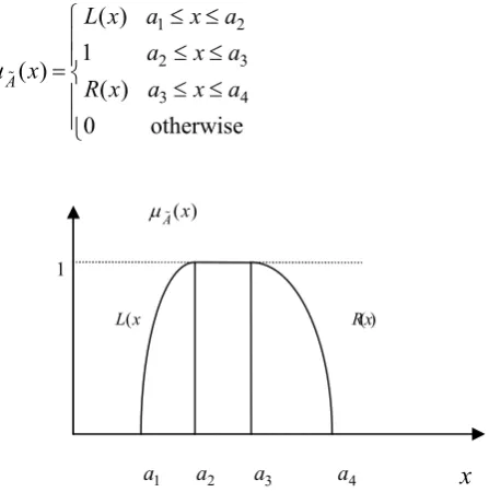
Generalized Fuzzy Number
The generalized fuzzy number
A
with membership function( )
A
x
(Figure 1) exhibits a fuzzy subset of the real line ,where
1 2
2 3
3 4
( )
1
( )
( )
0
otherwise
AL x
a
x
a
a
x
a
x
R x
a
x
a
[image:3.595.312.536.237.468.2]
Fig. 1. Generalized fuzzy number
where,
L x
( )
andR x
( )
are continuous functions of x. Moreover,L x
( )
is strictly monotonic increasing andR x
( )
strictly monotonic decreasing function of x in
a
1
x
a
2 and3 4
a
x
a
respectively.Defuzzification
Defuzzification is the process of producing a quantifiable result in fuzzy logic, given the fuzzy sets and the corresponding degrees of membership. There are several defuzzification techniques available in the existing literature. However, we have used the method of Centre of Approximated Interval (CAI).
Centre of the Approximated Interval (CAI)
Let
A
be a fuzzy number with interval of confidence at the level
, then the
-cut is[
A
L( ),
A
R( )]
. The nearest( ) A x
1
a a2 a3 a4
1
( )
L x R x( )
interval approximation of
A
with respect to the distance metricd
is 1 10 0
( ) ( ) , ( )
d L R
C A A d A d
,
where 1
2 1
20 0
( , ) L( ) L( ) R( ) R( ) .
d A B
AB d
AB dThe interval approximation for the trapezoidal fuzzy number
1 2 3 4
( , , , )
A a a a a is
(a1a2) / 2, (a3a4) / 2 .
Thus, we have,
1 2 3 4
CAI A a a a a / 4.
Problem formulation
According to assumption (i), the reliability of each component of a system is fuzzy number. So, the system reliability will be fuzzy valued. The redundancy at the modular (subsystem) level is considered rather than at the component level as the earlier one is more effective than the later one. Here, the series system and parallel redundancy are considered and also it is assumed that the failures are statistically independent. The optimal modular redundancy allocation is considered under the strict restriction that only one level among components, module and system can be available for redundancy. The proposed model is described after giving the meanings of the frequently used terms while reporting the model. The term ‘unit’ can be used commonly for subsystem, module and component. The unit A
is the parent unit of B if B is a unit of A and B is located at one lower level than A. If C is a unit of A, then A is an ‘ancestor’ unit of C. If D is a unit of A and D is located at one lower level than A, D is a ‘child’ unit of A. If E is a unit of A, E is a ‘offspring’ of A and if the parent unit of F and G are same, they are the ‘sibling’ units. If the levels of H and I are same, then they are ‘cousin’ units. The aim is to maximize the system reliability with suitable redundancy allocations as well as to fit the resource constraints. Here, the variable
x
j denotes thenumber of allocated unit j and
y
j indicates whether the unit jis actually used or not. Thus the actual number of allocated unit
j becomes(x yj. j). The constraint functions are constructed
depending upon the available resources such as cost, weight and volume. The constraint functions depending on weight and volume are regarded as linear interval functions and the corresponding cost is taken asC x( )cx x. The cost function
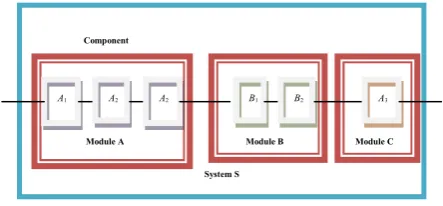
is the sum of the price cx and the additive cost xand it is clear that the additive cost increases geometrically as the redundancy increases. A hierarchical modular redundancy structure is shown in the Figure 2 below.
[image:4.595.50.272.631.734.2]
Fig. 2. System structure of modular redundancy
Considering the modular redundancy, the corresponding redundancy allocation problem is formulated as follows:
Maximize
1
(1 (1 ) )i
n
x
S i i
i
R x y r
(1)
subject to
1
( , , ) , 1, 2,....,
n
i pi i i i p p
i
y g x y r b p n
{ }
1
a
i k
k i
y y
0
i
y or 1 for all i and all xi1and i denotes the components in the lowest level.
The above problem is constrained optimization problem with interval valued objective.
Genetic algorithm based constraints handling technique
To solve the fuzzy valued constrained optimization problems, Genetic algorithm (GA) (Goldberg, 1989; Michalewicz, 1996; Sakawa, 2002; Deb, 2000) can be used for easy implementation of the global optimal solution. The constrained optimization problem is converted into unconstrained optimization problem with the help of penalty function technique given by Miettinen, Makela and Toivanen (2003) and Aggarwal and Gupta (2005). The aim of the penalty function technique is to penalize the infeasible solutions. Gupta, Bhunia and Roy (2009) proposed the Big-M penalty technique in which a large negative number (say –M, M being a large positive number) is penalized for infeasible solution of the problem and a new unconstrained optimization problem is formed. For this penalty technique, the reduced problem of problem (1) is as follows:
Maximize defuz R
S defuz R
S (2)where
0 if ( , , )
if ( , , ) i
S i
x y r S
defuz R M x y r S
( ,i i, ) :i pi( ,i i, )i i, 1, 2,...,
S x y r g x y r b i m andlxu,
wherel( , ,..., )l l1 2 lq ,u( ,u u1 2,...,uq),x( ,x x1 2,...,xn),
1 2
( , ,..., n) i 0 or 1, 1, 2,...,
y y y y y i n .
Problem (2) is a non-linear unconstrained optimization problem with fuzzy objective of n integer variables x x1, 2,...,xnand n binary variablesy y1, 2,...,yn. For solving this problem with 2n variables, we have developed a real coded genetic algorithm (GA) with advanced operators for integer as well as binary variables. Genetic Algorithm (GA) is a stochastic search and optimization technique (Goldberg 1989). Gen and Cheng (1996) described the application of GA to combinatorial problems including reliability optimization problems. Perhaps, GA is the most widely known evolutionary computation method due to its simplicity, powerfulness and wide application. It works by the evolutionary principles and chromosomal processing in natural genetics. GA maintains a
System S
Module C Module B
Module A Component
population P t
for generation t, of chromosomes which are the set of genes, the part of solution. The most fundamental idea of Genetic Algorithm is to replicate the natural evolution process artificially in which populations undergo continuous changes through genetic operators, like crossover, mutation and selection. In particular, it is very useful for solving complicated optimization problems which cannot be solved easily by direct or gradient based mathematical techniques. It is very effective to handle large-scale, real-life, discrete and continuous optimization problems without making unrealistic assumptions and approximations. The approach of GA is applied to many engineering problem as well as decision making problems in various fields. Some distinguishing characteristics of GA are as follows (Goldberg 1989):(i) GA works with a coding of solution set, not the solution themselves,
(ii) GA searches over a population of solutions, not a single solution,
(iii) GA uses payoff information, not derivatives or other auxiliary knowledge,
(iv) GA applies stochastic transformation rules, not deterministic.
Each chromosome represents a potential solution to the problem under consideration and is evaluated to give some measure of its fitness. Some chromosomes undergo stochastic transformation by means of genetic operators to form new chromosomes. The genetic operator ‘crossover’ creates new chromosomes by combining some parts from two chromosomes and the other genetic operator ‘mutation’ produces offspring by making changes in a single chromosome. A new population is formed by selecting the chromosomes having better fitness value from the parent and the offspring populations taken together. After several generations, the algorithm converges to the best chromosome having the best fitness value and it represents the optimal solution.
The algorithm for implementing GA is as follows:
Step-1: Set population size (ps), maximum number of
generations (mg), probability of crossover (pc),
probability of mutation (pm) and the bounds of
decision variables. Step-2: Set t=0.
Step-3: Initialize the chromosomes of the population P t
. Step-4: Compute the fitness function (objective function) foreach chromosome of P t
.Step-5: Find the chromosome having the best fitness value. Step-6: Set t=t +1.
Step-7: If the termination condition is satisfied go to Step-13; otherwise go to the next step.
Step-8: Select the population P t
from the population
1
P t of (t-1)- th generation using tournament selection.
Step-9: Apply crossover & mutation operators on P t
to produce new population P t
.Step-10: Compute the fitness function value of each chromosome of P t
.Step-11: Find the best chromosome from P t
.Step-12: Find the better of the best chromosomes of P t
&
1
P t and store it; go to Step-6.
Step-13: Print the best chromosome and its fitness value Step-14: End.
Basic components of genetic algorithm
(i) GA parameters (population size, maximum number of generation, crossover rate and mutation rate)
(ii) Chromosome representation (iii) Initialization of population (iv) Evaluation of fitness function (v) Selection process
(vi) Genetic operators (crossover, mutation and elitism)
GA parameters
For implementing GA we have considered the following GA parameters:
Population size (ps): Population size determines the amount of
information stored by the GA. There is no clear rule how large it should be. The population size is problem dependent and will need to increase/decrease with the dimension of the problem.
Maximum number of generations (mg): It varies from
problem to problem and depends upon the number of genes (variables) of a chromosome and it is being prescribed to be the termination criterion for convergence of the solution.
Probability of crossover (pc): In Genetic Algorithms
crossover is considered to be the main search operator. The crossover operator is used to thoroughly explore the search process. In crossover operator the genetic information between two or more individuals are blended to produce new individuals. Normal range of the crossover rate lies in [0.60, 0.95].
Probability of mutation (pm): Mutation operator plays an
important role in genetic algorithm. After crossover operation, mutation is performed. It is intended to prevent to the falling of all solutions in the population into a local optimum of the problem under consideration. Mutation operator randomly changes the offspring resulted from crossover. The mutation rate lies in [0.05, 0.20]. Sometimes mutation rate is considered to be 1/n where n is the number of genes (variables) of the chromosome.
Chromosome representation
floating point or combination of the both numbers and every component of that chromosome represents a decision variable of the problem. In this representation, each chromosome is encoded as a vector of integer numbers, with the same component as the vector of decision variables of the problem under consideration. This type of representation is accurate and more efficient as it is closed to the real design space and moreover, the string length of each chromosome is same as the number of decision variables. In this representation, for a given problem with n decision variables, a n-component vector
1 2
( , , , n)
x x x x is used as a chromosome to represent a solution to the problem. A chromosome denoted as vk (
1, 2,..., s)
k p is an ordered list of n genes as
1 2
{ , ,..., ,..., }
k k k ki kn
v v v v v .
Initialization of population
After representation of chromosome, the next step is to initialize the chromosome that will take part in the artificial genetics.To initialize the population, first of all we have to find the independent variables and their bounds for the given problem. Then the initialization process produces population size number of chromosomes in which every component for each chromosome is randomly generated within the bounds of the corresponding decision variable. There are several procedures for selecting a random numbers of integer types. In this work, we have used the following algorithm for selecting of an integer random number.
An integer random number between a and b can be generated as either xag or, x b g, where g is a random integer
between 1 and a b .
Evaluation of fitness function
Evaluation of fitness function is same for natural evolution process in the biological and physical environments. After initialization of chromosomes of potential solutions, we need to see how relatively good they are. Therefore, we have to calculate the fitness value for each chromosome. In our work, the value of objective function of the reduced unconstrained optimization problems corresponding to the chromosome is considered as the fitness value of that chromosome.
Selection of fitness function
The selection operator which is the first operator in artificial genetics plays an interesting role in GA. This selection process is based on the Darwin’s principle on natural evolution “survival of the fittest”. The primary objective of this process is to select the above average individuals/chromosomes from the population according to the fitness value of each chromosome and eliminate the rest of the individuals/chromosomes. There are several methods for implementing the selection process.
In this work, we have used tournament selection process of size two with replacement as the selection operator with the following assumptions:
(i) If both the chromosomes/individuals are feasible, then the chromosome with better fitness value is selected.
(ii) If one feasible and another infeasible chromosome/ individual are considered then the feasible chromosome is selected.
(iii) For both infeasible chromosomes/individuals with unequal constraints violation, the chromosome with less constraints violation is selected.
(iv) For both infeasible chromosomes/individuals with equal constraints violation, any one chromosome/individual is selected.
Genetic operators
After the selection process, other genetic operators, like crossover and mutation are applied to the resulting chromosomes those which have survived. Crossover is an operator that creates new individuals/chromosomes (offspring) by combining the features of both parent solutions. It operates on two or more parent solutions at a time and produces offspring for next generation. In this work, we have used intermediate crossover for integer variables.
The aim of mutation operator is to introduce the random variations into the population and is used to prevent the search process from converging to the local optima. This operator helps to regain the information lost in earlier generations and is responsible for fine tuning capabilities of the system and is applied to a single individual only. Usually, its rate is very low; because otherwise it would defeat the order building being generated through the selection and crossover operations. In this work we have used one-neighborhood mutation.
Elitism preserves and uses the best chromosome obtained in the previous generations. To overcome the situation that the best chromosome may be lost when a new population is generated by crossover and mutation operations, the worst individual/chromosome is replaced by the best individual/chromosome in the current generation. In this operation, one or more chromosomes may take part.
Numerical Examples and Sensitivity analysis
To illustrate the performance of the proposed method in solving modular redundancy allocation problem in interval environment we have performed numerical experiments considering an example.
For this purpose, we have developed Genetic Algorithm considering fuzzy fitness value and defuzzification method.
This algorithm is coded in C++ programming language and the numerical computations are carried out in a PC with Intel i5 processor in LINUX environment.
For each case 100 independent runs have been performed to calculate the best found results viz., the system reliability and the system cost.
The values of GA parameters used in the experiments are as follows:
Fig. 3. Modular System in the Example
Example: In this example, a series system (Fig 3) is considered and the corresponding numerical data are given in Table 1. The cost availability is taken to be fuzzy valued where,
(225, 235, 245,255)
C . For this example 100 independent runs have been performed and the best found results with fuzzy parameters and fixed parameters are presented in Table 2.
1 11
13 12
111 112
113 121
1 1 11 11
12 12 13 13
111 111 112 112
113 113 121 121
Max (1 (1 ) )(1 (1 ) )
(1 (1 ) )(1 (1 ) )
(1 (1 ) )(1 (1 ) )
(1 (1 ) )(1 (1 ) )
x x S x x x x x x
R y r y r
y r y r
y r y r
y r y r
131 122 132
122 122 131 131
132 132
(1 (1 ) )(1 (1 ) )
(1 (1 ) )
x x
x
y r y r
y r subject to 1 11 12 13 111 112 113 121
1 1 1 1 11 11 11 11
12 12 12 12 13 13 13 13
111 111 111 111 112 112 112 112
113 113 113 113 121 121 121 121
122 122 122
( ) ( ) ( ) ( ) ( ) ( ) ( ) ( ) ( x x x x x x x x
y c x y c x
y c x y c x
y c x y c x
y c x y c x
y c x
122 131
132
122 131 131 131 131
132 132 132 132
) ( )
( )
x x
x
y c x
y c x C
1 11 111 1
y y y
1 11 112 1
y y y
1 11 113 1
y y y
1 12 121 1
y y y
1 12 122 1
y y y
1 13 131 1
y y y
1 13 132 1
y y y
0 or 1
j
y j
1
i
x i and integer.
[image:7.595.308.555.215.391.2]For solving the optimization problems, the GA based penalty approach has been used. In this approach, -M (M being a large number) is considered for the value of the fitness function corresponding to infeasible solution. Gupta, Bhunia and Roy (2009) applied this
Table 1. Numerical Data
Basic item Parent
item ri ci i
S – (0.30,0.35,0.45, 0.50) (69,71,73,75) (0,1,3,5)
A S (0.60,0.65,0.70, 0.75) (20,23,25,28) (0,1,3,5)
B S (0.65,0.70,0.75, 0.78) (16,18,20,22) (1,2,4,6)
C S (0.62,0.66,0.72, 0.76) (18,22,23,25) (0,1,3,5) 1
A A (0.80,0.85,0.91, 0.96) (2,4,6,8) (1,2,4,6)
2
A A (0.85,0.89,0.97, 0.99) (3,5,7,9) (1,3,5,7)
3
A A (0.80,0.82,0.86, 0.89) (3,5,7,9) (1,3,5,7)
1
B B (0.82,0.86,0.92, 0.95) (3,5,7,9) (2,3,5,7)
2
B B (0.81,0.83,0.86, 0.90) (2,4,6,8) (1,2,5,6)
1
C C (0.82,0.85,0.92, 0.96) (4,7,8,9) (1,2,4,5)
2
C C (0.75,0.78,0.81, 0.86) (4,6,8,10) (2,3,5,7)
Table 2. Best found results
i1, 2,,11
Parameters .
i i
xy x R Cost
Fixed * 0,0,3,3,2,2,2,0,0,0,0 0.931863 228.00 Interval ** 0,0,3,3,2,2,2,0,0,0,0 [0.890774,
0.974029]
[216.00, 240.00] Fuzzy 0,0,0,3,3,2,2,2,2,0,0 0.906443 225.00
* Yun et al. (2004) , **Sahoo et al (2015)
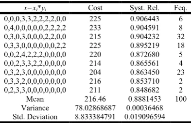
Table 3. Best found results from 100 runs
i1, 2,,11
x=xi*yi Cost Syst. Rel. Feq.
0,0,0,3,3,2,2,2,2,0,0 225 0.906443 6 0,4,0,0,0,0,0,2,2,2,2 233 0.904591 8 0,3,0,3,0,0,0,2,2,0,0 215 0.904232 32 0,3,3,0,0,0,0,0,0,2,2 225 0.895219 18 0,0,2,4,2,2,2,0,0,0,0 220 0.872680 5 0,0,2,3,3,2,2,0,0,0,0 214 0.865561 4 0,3,2,3,0,0,0,0,0,0,0 204 0.863450 23 0,3,3,2,0,0,0,0,0,0,0 216 0.853710 2 0,2,3,3,0,0,0,0,0,0,0 211 0.848682 2 Mean 216.46 0.8881453 100 Variance 78.02868687 0.00036468 Std. Deviation 8.833384791 0.019096594
for solving constrained reliability optimization problems. In their works there is no indication regarding the value of M. However, for infeasible solution the value of M may be taken depending on the fitness function value. In case of maximization problem, a small value and in case of minimization problems a large value may be considered for M
[image:7.595.324.541.430.493.2] [image:7.595.335.532.535.662.2]Result Analysis
[image:8.595.311.557.51.211.2]To study the performance of the proposed method for solving modular reliability allocation problem, sensitivity analyses have been performed graphically for system reliability with respect to different GA parameters separately by changing one parameter at a time and keeping the other at their original value.
[image:8.595.37.290.158.300.2]Fig. 4. Graphical representation of frequency of Cost & System Reliability
Fig. 5. Cost vs. System Reliability
The graphical representation of the analysis has been shown in Fig 4-6. The Fig 4 represents the system reliability with regard to system cost and system reliability. In figure 5, we can see the curve of variation of system reliability with respect to the system cost. The frequency distribution of the system reliability out of 100 runs is presented in table 3 and also by
The best found result is presented in the table 2
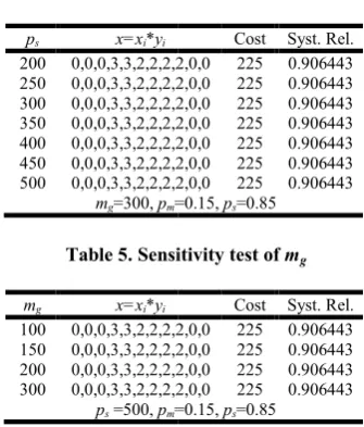
comparisons with the available results are also presented. Table 3 represents the frequency table of the best found outcomes from 100 runs along with the computation of mean, variance & standard deviation of the system reliability. It is to be noted from table 4 that the result is stable for wide range of
from 200 to 500. Sensitivity of mg (varying from 100 to 300)
has been reported in Table 5.
Also, we have observed the stability of the system reliability with respect to the parameters pc (varied from 0.5 to 0.95) and
the pm (varied from 0.01 to 0.3).
rformance of the proposed method for solving modular reliability allocation problem, sensitivity analyses have been performed graphically for system reliability with respect to different GA parameters separately by changing one ing the other at their original
Graphical representation of frequency of Cost & System
Cost vs. System Reliability
The graphical representation of the analysis has been shown in represents the system reliability with regard to system cost and system reliability. In figure 5, we can see the curve of variation of system reliability with respect to the system cost. The frequency distribution of the system reliability
is presented in table 3 and also by Figure 6.
The best found result is presented in the table 2, where the comparisons with the available results are also presented. Table 3 represents the frequency table of the best found outcomes ith the computation of mean, variance & standard deviation of the system reliability. It is to be noted from table 4 that the result is stable for wide range of ps varying
(varying from 100 to 300)
Also, we have observed the stability of the system reliability (varied from 0.5 to 0.95) and
[image:8.595.348.516.256.453.2]Fig. 6. Frequency distribution of System Reliability
Table 4. Sensitivity test of
ps x=xi*yi
200 0,0,0,3,3,2,2,2,2,0,0 250 0,0,0,3,3,2,2,2,2,0,0 300 0,0,0,3,3,2,2,2,2,0,0 350 0,0,0,3,3,2,2,2,2,0,0 400 0,0,0,3,3,2,2,2,2,0,0 450 0,0,0,3,3,2,2,2,2,0,0 500 0,0,0,3,3,2,2,2,2,0,0
mg=300, pm=0.15,
Table 5. Sensitivity test of
mg x=xi*yi
100 0,0,0,3,3,2,2,2,2,0,0 150 0,0,0,3,3,2,2,2,2,0,0 200 0,0,0,3,3,2,2,2,2,0,0 300 0,0,0,3,3,2,2,2,2,0,0
ps =500, pm=0.15,
Conclusion
The importance of modular redundancy allocation applied to multilevel system reliability problems in fuzzy environment is treated in this paper. Here,
redundancy allocation problem in series system with parallel redundancy considering trapezoidal fuzzy values for the reliability of each component and for the involved parameters also. Then CAI method is applied for
values so that to convert into deterministic form. After that Big-M penalty technique is used to convert the problem into unconstrained one. The transformed problem then solved with the help of advanced genetic algorithm. To solve th
other heuristic methods like simulated annealing, tabu search, ant system, particle swarm optimization etc. can be applied. For future studies, one may formulate and solve other type of modular redundancy allocation problems for series
system, multi-objective case, etc.
Acknowledgement
The authors wish to express his thanks to Dr. A. K. Bhunia, Professor, Department of Mathematics, The University of Burdwan, for his suggestion to investigate the computational aspects of our problem and for his frequent valuable suggestions.
Frequency distribution of System Reliability
Sensitivity test of ps
Cost Syst. Rel. 0,0,0,3,3,2,2,2,2,0,0 225 0.906443 0,0,0,3,3,2,2,2,2,0,0 225 0.906443 0,0,0,3,3,2,2,2,2,0,0 225 0.906443 0,0,0,3,3,2,2,2,2,0,0 225 0.906443 0,0,0,3,3,2,2,2,2,0,0 225 0.906443 0,0,0,3,3,2,2,2,2,0,0 225 0.906443 0,0,0,3,3,2,2,2,2,0,0 225 0.906443
=0.15, ps=0.85
Sensitivity test of mg
Cost Syst. Rel. 0,0,0,3,3,2,2,2,2,0,0 225 0.906443 0,0,0,3,3,2,2,2,2,0,0 225 0.906443 0,0,0,3,3,2,2,2,2,0,0 225 0.906443 0,0,0,3,3,2,2,2,2,0,0 225 0.906443
=0.15, ps=0.85
The importance of modular redundancy allocation applied to multilevel system reliability problems in fuzzy environment is we have formulated modular redundancy allocation problem in series system with parallel redundancy considering trapezoidal fuzzy values for the reliability of each component and for the involved parameters also. Then CAI method is applied for defuzzfying the fuzzy values so that to convert into deterministic form. After that M penalty technique is used to convert the problem into The transformed problem then solved with the help of advanced genetic algorithm. To solve the problems, other heuristic methods like simulated annealing, tabu search, ant system, particle swarm optimization etc. can be applied. For future studies, one may formulate and solve other type of modular redundancy allocation problems for series-parallel
objective case, etc.
[image:8.595.39.289.341.495.2]REFERENCES
Aggarwal, K.K. and Gupta, J.S. 2005. Penalty function approach in heuristic algorithms for constrained. IEEE
Transaction on Reliability, 54, 549-558.
Bhunia, A. K., Sahoo, L. and Roy, D. 2010. Reliability stochastic optimization for a series system with interval component reliability via genetic algorithm. Applied
Mathematics and Computations, 216, 929-939.
Boland, P. J. and El-Neweihi, E. 1995. Component redundancy vs. system redundancy in the hazard rate ordering. IEEE
Transaction on Reliability, 44, 614-619.
Deb, K. 2000. An efficient constraint handling method for genetic algorithms. Computer Methods in Applied
Mechanics and Engineering, 186, 311-338.
Goldberg, D.E. 1989. Genetic Algorithms: Search,
Optimization and Machine Learning. Reading, MA:
Addison Wesley.
Gupta, R. K., Bhunia, A. K. and Roy, D. 2009. A GA Based penalty function technique for solving constrained Redundancy allocation problem of series system with interval valued reliabilities of components. Journal of
Computational and Applied Mathematics, 232, 275-284.
Hansen, E. and Walster, G. W. 2004. Global optimization using
interval analysis. New York: Marcel Dekker Inc.
Karmakar, S., Mahato, S. and Bhunia, A. K. 2009. Interval oriented multi-section techniques for global optimization.
Journal of Computational and Applied Mathematics, 224,
476-491.
Kumar, R., Izui, K., Yoshimura, M. and Nishiwaki, S. 2009. Optimal multilevel redundancy allocation in series and series-parallel systems. Computers and Industrial
Engineering, 57, 169-180.
Mahato, S. K. and Bhunia, A. K. 2006. Interval-arithmetic-oriented interval computing technique for global optimization. Applied Mathematics Research Express, 2006, 1-19.
Michalewicz, Z. 1996. Genetic Algorithms + Data structure =
Evoluation Programs. Berlin, Springer Verlag.
Miettinen, K., Makela, M. M. and Toivanen, J. 2003. Numerical comparison of some penalty-based constraint handling techniques in genetic algorithms. Journal of
Global Optimization, 27, 427-446.
Moore, R. E. 1979. Methods and applications of interval
Analysis. SIAM.
Rasmussen, N. and Niles, S. 2005. Modular systems: The
evolution of reliability. White paper, American Power
Corporation.
Sahoo, L., Bhunia, A. K. and Kapur, P. K. 2012. Genetic algorithm based multi-objective reliability optimization in interval environment. Computers and Industrial
Engineering, 62, 152-160.
Sahoo, L., Bhunia, A. K. and Roy, D. 2010. A genetic algorithm based reliability redundancy optimization for interval valued reliabilities of components. Journal of
Applied Quantitative Methods,5, 270-287.
Sahoo, L., Mahato, S.K. and Bhunia, A. K. 2015. Multi-Level Reliability Redundancy Allocation Problem in Interval Environment via Genetic Algorithm. Communications in Dependability and Quality Management-An International
Journal, 18(1), 65-80.
Sakawa, M. 2002. Genetic Algorithms and fuzzy multiobjective
optimization. Kluwer Academic Publishers.
Yun, W. Y. and Kim, J. W. 2004. Multi-level redundancy optimization in series systems. Computers and Industrial
Engineering, 46, 337-346.
Yun, W. Y., Song, Y. M. and Kim, H. G. 2007. Multiple multi-level redundancy allocation in series system. Reliability
Engineering and System Safety, 92, 308-313.