Energy Efficient Path Determination in Wireless Sensor Network Using BFS Approach

doi:10.4236/wsn.2011.311040 Published Online November 2011 (http://www.SciRP.org/journal/wsn)

Energy Efficient Path Determination in Wireless Sensor

Network Using BFS Approach

Shilpa Mahajan1, Jyoteesh Malhotra2 1

CSE, ITM University, Gurgaon, India 2

ECE, GNDU, Amritsar, India

E-mail: [email protected], [email protected]

Received September 9, 2011; revised October 10, 2011; accepted October 20, 2011

Abstract

The wireless sensor networks (WSN) are formed by a large number of sensor nodes working together to pro-vide a specific duty. However, the low energy capacity assigned to each node prompts users to look at an important design challenge such as lifetime maximization. Therefore, designing effective routing techniques that conserve scarce energy resources is a critical issue in WSN. Though, the chain-based routing is one of significant routing mechanisms but several common flaws, such as data propagation delay and redundant transmission, are associated with it. In this paper, we will be proposing an energy efficient technique based on graph theory that can be used to find out minimum path based on some defined conditions from a source node to the destination node. Initially, a sensor area is divided into number of levels by a base station based on signal strength. It is important to note that this technique will always found out minimum path and even alternate path are also saved in case of node failure.

Keywords:Graph Theory, Breadth First Search, Energy Efficient, Cost, Shortest Path

1. Introduction

A wireless sensor network (WSN) is a specialized wire-less network that is composed of a number of sensor nodes deployed in a specified area for monitoring envi-ronment conditions such as temperature, air pressure, humidity, light, motion or vibration, and so on. The sen-sor nodes are usually programmed to monitor or collect data from surrounding environment and pass the infor-mation to the base station for remote user access through various communication technologies. Typically, a sensor node is a small device that consists of four basic compo-nents 1) sensing subsystem for data gathering from its environment, 2) processing subsystem for data process-ing and data storprocess-ing, 3) wireless communication subsys-tem for data transmission and 4) energy supply subsystem which is a power source for the sensor node. However, sensor nodes have small memory, slow processing speed, and scarce energy supply. These limitations are typical characteristics of sensor nodes which effects, sensor networks life and the quality . For that reason, the proto-cols running on sensor networks must consume the re-sources of the nodes efficiently in order to achieve a

longer network lifetime. There is an ongoing research on power organization issues in order to reduce the power u- tilization when the nodes become idle[1,2]. When power efficient communication is considered, it is important to maximize the nodes lifetimes, reduce bandwidth require- ments by using local collaboration among the nodes, and tolerate node failures, besides delivering the data effi-ciently.

An efficient routing technique is required to design a network in a way to efficiently utilize the energy of nodes to prolong the lifetime of the network. Since com- munication consume significant amount of battery power, sensor nodes should spend as little energy as possible when receiving and transmitting data [3-5]. Network life- time can be increased by reducing bandwidth consump-tion by using local collaboraconsump-tion among nodes and toler-ate node failures [6].

1.1. Background

The earliest and simple approach was direct transmission in which each sensor node will sense & transmit its data to BS individually. Since base station is located far away from sensor nodes resulting higher transmission cost. Because of this high cost transmission the energy of nodes drain off faster and thus having short system life-time. In order to solve the problem, clustering based pro- tocols were proposed where a cluster is a group of sensor nodes, with a head node managing all other member nodes. The heads are responsible for coordinating mem-ber nodes, gathering data within the clusters, aggregating data and forwarding the aggregated data to the base sta-tion.

LEACH [7] is a cluster-based, distributed, autono-mous protocol. The algorithm randomly chooses a por-tion of the sensor nodes as cluster heads, and lets the remaining sensor nodes choose their nearest heads to join. The cluster member’s data is transmitted to the head, where the data is aggregated and further forwarded to the base station. The LEACH algorithm reduces the number of nodes that directly communicate with the base station. It also reduces the size of data being transmitted to the base station. Thus, LEACH greatly saves communication energy. Since the protocol randomly chooses cluster heads in each round, the energy consumption is theoreti-cally evenly distributed among all sensor nodes data ag-gregation techniques in WSN. They are clustering based [4], tree-based [8], and chain-based [9]. In this section, we only review three chain-based routing protocols, PEGASIS [9], COSEN [10], and Enhanced PEGASIS [9], and point out their pros and cons.

A)PEGASIS

PEGASIS is a basic chain-based routing protocol [9]. In which, all nodes in the sensing area are first organized into a chain by using a greedy algorithm, and then take turns to act as the chain leader. In data dissemination phase, every node receives the sensing information from its closest upstream neighbor, and then passes its aggre-gated data toward the designated leader, via its down-stream neighbor, and finally the base station.

Although the PEGASIS constructs a chain connecting all nodes to balance network energy dissipation, there are still some flaws with this scheme. 1) For a large sensing field and real-time applications, the single long chain may introduce an unacceptable data delay time. 2) Since the chain leader is elected by taking turns, for some cases, several sensor nodes might reversely transmit their ag-gregated data to the designated leader, which is far away from the BS than itself. This will result in redundant transmission paths, and therefore seriously waste net-work energy. 3) The single chain leader may become a

bottleneck. B) COSEN

In contrast to PEGASIS, COSEN [10] is a two-tier hi-erarchical chain-based routing scheme. In that scheme, sensor nodes are geographically grouped into several low- level chains. For each low-level chain, the sensor node with the maximum residual energy is elected as the chain leader.

C)Enhanced PEGASIS

In 2007, Jung et al. proposed a variation of PEGASIS routing scheme, termed as Enhanced PEGASIS [11]. In their method, the sensing area, centered at the BS, is cir-cularized into several concentric cluster levels. For each cluster level, based on the greedy algorithm of PEGASIS, a node chain is constructed. In data transmission, the common nodes also conduct a similar way as the PEGA- SIS to transfer their sensing data to its chain leader.

D) CHIRON

Chain-Based Hierarchical Routing Protocol, named as CHIRON [12], based on the Beam Star concept [9], the main idea of CHIRON is to split the sensing field into a number of smaller areas, so that it can create multiple shorter chains to reduce the data transmission delay and redundant path, and therefore effectively conserve the node energy and prolong the network lifetime.

E) PEDAP

In PEDAP (Power Efficient and Data gathering and Aggregation Protocol), Chain is formed based on mini-mum spanning tree and minimini-mum energy concept [13].

F) CCPAR

The basic idea of CCPAR i.e. Clustered Chain based Power Aware Routing Scheme for Wireless Sensor Net- works scheme is that the nodes within a cluster are con-nected in a chain and each node receives from and tran- smits to the closest neighbors in the chain [14].This tech- nique provide greater reduction in energy consumption and thus increases the life time.

2. Proposed Algorithm

2.1. Level Assignment

First, sensor network area says M*M will be divided in to number of concentric circles defined as levels. Each node in the sensor networks is assigned its own level based on signal strength from the base station. The num-bers of these levels depend on various parameters such as density of the sensor network, the number of nodes or the location of the base station as shown in Figure 1.

Level-1 Level-2 Level-3 Level-4

Figure 1. Level assignment.

concept of numbering we can even assign ID to each node like A, B, C, D etc.

2.2. Route Discovery Phase

Route discovery is based on query and reply cycles, and route information is stored in all intermediate nodes along the route in the form of route table entries. Since nodes do not have any route information, the route dis-covery process can be initiated by each node by sending a route request packet, to find neighboring nodes those are one hop away from it .A source node will maintain routing table containing information shown in Figure 2.

Each node can get to know its neighborhood by using local broadcasts, so-called HELLO message. Nodes neigh- bors are all the nodes that it can directly communicate with.

The HELLO messages will never be forwarded be-cause they are broadcasted with TTL = 1. After a mes-sage has been broadcasted, a node will wait for route re- ply message. As soon as source node receives route reply message from nodes, it will update its routing table entry destination ID. Sequence number will keep account of the fresh routes. Battery status will give information re-garding energy levels of the nodes. Visit field will help in tracing a route from a source point to a destination node. We will use the TTL =1, in order to find neigh- boring nodes who are one hope away. Only those nodes who have there energy level greater than defines thresh-old level will take part in data transfer phase.

2.3. Breadth First Search Approach:

In graph theory, breadth-first search (BFS) is a graph search algorithm [15] that begins at the root node and explores all the neighboring nodes. Then for each of those nearest nodes, it explores their unexplored neighbor nodes, and so on, until it finds the goal. It has been proved by induction that the breadth first search tree is a shortest path tree starting from its root. Every vertex has a path to the root, with path length equal to its level (just follow the tree itself), and no path can skip a level so this really is a shortest path.

Source ID

Destination ID

Node_ Status

Sequence nos

Battery Status

Visit TTL

Figure 2. Routing table.

Process:

This algorithm uses queue to store the nodes of each level of the graph as they are visited .These stored nodes are then treated one by one and their adjacent nodes are visited .These stored nodes have been visited. This ter-minating condition is reached when the queue is empty. There are three states that are defined with respect to current node status. The field Node-Status will keep ac-count of the states of the nodes.

A node that has not been visited yet and waiting to be processed , will be in ready state .In the beginning all nodes will be in ready state .As soon as the node is added on to queue ,it will be waiting state.

The node that has been processed i.e. whose neighbors have been added on to queue will be in processed state. Nodes that have been processed once will not be consid-ered again. So the field visit in a table will keep account of it. In the beginnings all node will have zero in visit field as soon as a node is visited the value get updated to 1.

2.3.1. Table Construction

In the beginning phase, a route discovery will be initiated, all nodes will update their routing table keeping in all details .At this time visit field will be 0.Since, the cost of sensing is less as compare to cost of communication.

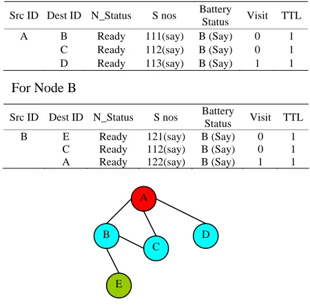
For example consider a tree of nodes as shown in Fig-ure 3.

In the Beginning: For Node A

Src ID Dest ID N_Status S nos Battery

Status Visit TTL

A B Ready 111(say) B (Say) 0 1

C Ready 112(say) B (Say) 0 1

D Ready 113(say) B (Say) 1 1

For Node B

Src ID Dest ID N_Status S nos Battery

Status Visit TTL

B E Ready 121(say) B (Say) 0 1

C Ready 112(say) B (Say) 0 1

A Ready 122(say) B (Say) 1 1

A

B

C

D

E

All nodes will update their routing table accordingly in the initialization phase. After this, a route discovery phase will start from the farthest node say base station in wire-less sensor network field. Queue will be maintained, the staring node say A will be in processed state and all other like B,C,D are in waiting state.

Src ID Dest ID N_Status S nos Battery

Status Visit TTL

A B Waiting 111(say) B (Say) 1 1

C Waiting 112(say) B (Say) 1 1

D Waiting 113(say) B (Say) 1 1

Like wise when Node B will be processed from Queue

Src ID Dest ID N_Status S nos Battery

Status Visit TTL

B E Waiting 121(say) B (Say) 1 1

C Waiting 112(say) B (Say) 1 1

A Waiting 122(say) B (Say) 1 1

Once all the nodes have updated table details with sig-nificant data. Breath first search algorithm will be cal- led .Various steps for the algorithm is:

Algorithm BFS(G)

Step 1: Initialize all nodes to ready state (status =1) [Here n can be defined as the number of nodes. Ini-tially]*

visit =0

For (i=1; I <= n; i++) Visit[i] =0;

Step 2: Put the starting node in queue and change its status to the waiting state (status =2)

[Initialize starting node say v and make visit[v] =1]* [Add on to queue [v], initialize to pointers to keep track] Of front and rear element of queue

Front=Rear=–1 [initially]*

Rear=front=0 [incremented]* [Rear++, front++]*

Queue [Rear]= v

Step 3: Repeat step 4 and 5 until queue is empty [Check while (front<=Rear)]*

Step 4: Remove the front node n of queue. Process n and change the status of n to the processed state (status =3)

[Deleting element from the queue]* v = queue [front]

front++ //incrementing front by one

Step 5: Add to the rear of the queue all the neighbors of n that are in ready state (status =1), and change their

status to the waiting state (status =2). [End of the step 3 loop]

[find out all the nodes adjacent to v]* For (i=0; i<=n; i++)

Adj[v][i]==1 and visited[i]==0 Rear++

Queue[Rear]=i Step 6: Exit

2.4. Implementation

Assumptions:

1) All nodes have same and adequate amount initial energy.

2) A node can trust each other and there is no mali-cious intruder.

3) Each node or sink has ability to transmit message to any other node and sink directly.

4) Each sensor node has radio power control; node can tune the magnitude according to the transmission dis-tance.

5) Each sensor node has location information.

6) Every sensor nodes are fixed after they were de-ployed.

7) WSNs would not be maintained by humans. 8) Wireless sensor nodes are deployed densely and randomly in sensor field.

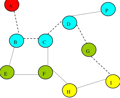
This concept can be explained by taking an example of 10 nodes and finding a path from a given node to a des-tination node as shown in Figure 4.

We have considered a network of 10 nodes .The nodes have been leveled based on the signal strength from the base station .A base station is the furthest node .Each Node has updated routing table keeping an account of nodes that are one hop away from it.

So the adjacency list will be:

A

B C

D

E

G

F

P

I

H

NODES Adjacent List

A B B C,E C B,D,F D C,G,P E B,F G D,I H F,I I G,H P D F C,H

Once this list has been created, A BFS approach can be used to find the minimum connected path/Spanning tree from a furthest node to a destination node as in Fig-ure 4 say (to find a path from A to I). While applying this algorithm, we will also keep account of the origin node

 A: B

Origin: A  B: C, E

Origin: B, B  C: E,D,F Origin: B,C,C

 E: D,F Origin: C,C

 D: F,G,P

Origin: A,D,D  F: G,P,H

Origin: D,F,F  G: P,H,I Origin: F,F,G

 P: H,I

Origin: F,G  H: I

Origin: G  I: - Origin: -

Considering nodes with their origin nodes; A,B,C,E,D,F,G,P,H,I

Ø,A,B,B,C,D,D,F,G Path selected will be

A->B->C->D->G->I

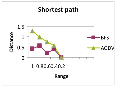
2.5. Simulation

A simulation of BFS has been done on mat lab 7.0 con-sidering a random network of 10 nodes. A trusted path distance has been calculated and is compared with AODV hop by hop network of 10 nodes .A graph has been plotted considering different ranges and corre-sponding distances has been plotted. All the assumptions discussed above have been kept in mind while perform-ing a simulation.

Shortest

path

0 0.5 1 1.5

1 0.80.60.40.2

Range

Dist

an

ce _BFS

AODV

Graph 1. Distance vs range

3. Conclusions

In this approach, nodes in the network are stationary and in next round when a node has a data to send to some other destined node, there is no need to create a routing table again and again until nodes have energy greater than threshold level. Only those nodes that are selected will be active and other nodes that don’t take part will remain in sleep mode. Nodes who have their energy less than threshold will not participate and thus in those cases the routing table has to be maintained again. This ap-proach will always result in finding the shortest path from a base station to a destined node. In future this method can be in corporate with MAC layer issues. Also, more comparisons study can be done with other proto-cols.

4. References

[1] D. Estrin, R. Govindan, J. Heidemann and S. Ku- mar, “Next Century Challenges: Scalable Coordination in Sensor Networks,” Proceedings of the Fifth Annual In-ternational Conference on Mobile Computing and Net-works 99, Seattle, 15-19 August 1999, pp. 263-270. [2] J. Kulik, W. Rabiner and H. Balakrishnan, “Adaptive

Protocols for Information dissemination in Wireless Sen-sor Networks,” Proceedings of the Fifth Annual Interna-tional Conference on Mobile Computing and Networks, Seattle, 15-18 August 1999, pp. 83-90.

[3] W. Mangione-Smith and P.S. Ghang, “A Low Power Medium Access Control Protocol for Portable Multi-Media Systems,” In Proceedings 3rd In- terna-tional Workshop on Mobile Multimedia Com- munica-tions, Princeton, September 1996, pp. 25-27.

[4] K. M. Sivalingam, M. B. Srivastava and P. Agrawal, “Low Power Link and Access Protocols for Wireless Multimedia Networks,” In Proceedings IEEE Vehicular Technology Conference, Phoenix, 4-7 May 1997, pp. 1331-1335.

“Reduc-ing Power Consumption of Network Interfaces in Hand-Held Devices,” In Proceedings 3rd International Workshop on Mobile Multimedia Communications, Prin- ceton, September 1996, pp. 25-27

[6] G. Bathla and G. Khan, “Energy-Efficient Routing Pro-tocol for Homogeneous Wireless Sensor Networks,” In-ternational Journal on Cloud Computing: Services and Architecture (IJCCSA), Vol. 1, No. 1, 2011.

[7] W. R. Heinzelman, A. Chandrakasan and H. Bala- krishnan, “Energyefficient Communication Protocol for Wireless Microsensor Networks,” In 33rd Annual Hawaii Interna-tional Conference on System Sciences, Hawaii, 4-7 Janu-ary 2000, pp. 3005-3014.

doi:10.1109/HICSS.2000.926982

[8] S. Hussain and O. Islam, “An Energy Efficient Span-ning Tree Based Multi-Hop Routing in Wireless Sensor Networks,” Proceedings of Wireless Communications and Networking Conference, Hong Kong, 11-15 March 2007, pp. 4383-4388. doi:10.1109/WCNC.2007.799

[9] S. Lindsey, C. S. Raghavendra and K. M. Sivalingam, “Data Gathering Algorithms in Sensor Networks Using Energy Metrics,” IEEE Transactions on Parallel Distrib-uted System, Vol. 13, No. 9, 2002, pp. 924-935.

doi:10.1109/TPDS.2002.1036066

[10] N. Tabassum, Q. E. K. M. Mamun and Q. Urano,

“COSEN: A Chain Oriented Sensor Network for Efficient Data Collection,” Proceedings of the Global Tlecommu-nications Conference, San Francisco, 1-5 December 2003, pp. 3525-3530.

[11] S. M. Jung, Y. J. Han and T. M. Chung, “The Concentric Clustering Scheme for Efficient Energy Consumption in the PEGASIS,” Proceedings of the 9th International Conference on Advanced Communication Technology, Phoenix, 12-17 February 2007, pp. 260-265.

doi:10.1109/ICACT.2007.358351

[12] K.-H. Chen, J.-M. Huang and C.-C. Siao, “An En-ergy-Efficient Chain-Based Hierarchical Routing Proto-col in Wireless Sensor Networks,” June 2009.

[13] H. O. Tan and I. Korpeoglu, “Power Efficient Data Gath-ering and Aggregation in Wireless Sensor Networks,”

ACM SIGMOD Record, Vol. 32, No. 4, 2003, pp. 66-71. doi:10.1145/959060.959072

[14] K. Majumder, “Clustered Chain Based Power Aware Routing Scheme for Wireless Sensor Networks,” Interna-tional Journal on Computer Science and Engineering, Vol. 2, No. 9, 2010, pp. 2953- 2963