Harmonic Analysis in Discrete Dynamical Systems
Gerardo Pastor1*, Miguel Romera1, Amalia Beatriz Orue1, Agustin Martin1, Marius F. Danca2, Fausto Montoya1
1
Instituto de Seguridad de la Información, CSIC, Madrid, Spain 2
Romanian Institute of Science and Technology, Cluj-Napoca, Romania Email: *[email protected]
Received February 7,2012; revised March 9, 2012; accepted March 192012
ABSTRACT
In this paper we review several contributions made in the field of discrete dynamical systems, inspired by harmonic analysis. Within discrete dynamical systems, we focus exclusively on quadratic maps, both one-dimensional (1D) and two-dimensional (2D), since these maps are the most widely used by experimental scientists. We first review the appli-cations in 1D quadratic maps, in particular the harmonics and antiharmonics introduced by Metropolis, Stein and Stein (MSS). The MSS harmonics of a periodic orbit calculate the symbolic sequences of the period doubling cascade of the orbit. Based on MSS harmonics, Pastor, Romera and Montoya (PRM) introduced the PRM harmonics, which allow to calculate the structure of a 1D quadratic map. Likewise, we review the applications in 2D quadratic maps. In this case both MSS harmonics and PRM harmonics deal with external arguments instead of with symbolic sequences. Finally, we review pseudoharmonics and pseudoantiharmonics, which enable new interesting applications.
Keywords: Harmonic Analysis; Discrete Dynamical Systems; MSS Harmonics; PRM Harmonics; Pseudoharmonics
1. Introduction
In this paper we review a branch of harmonic analysis applied to discrete dynamical systems. In general, har- monic analysis has been widely used in experimental applications, as in the field of signal processing. In the same way, harmonic analysis applied to discrete dy- namical systems can be a valuable tool for experimental scientists studying nonlinear phenomena. This paper is focused above all in showing some tools with interesting applications in nonlinear phenomena.
At its inception, the harmonic analysis studies the rep- resentation of a function as the superposition of basic waves which, in physics, are called harmonics. Fourier analysis and Fourier transforms are the two main branches investigated in this field. The harmonic analysis is soon generalized and in the past two centuries becomes, as noted above, a wide subject with a large number of appli- cations in diverse areas of experimental science.
In order to study nonlinear phenomena, experimental scientists use dynamical systems, whether continuous or discrete. In this review paper we only deal with discrete dynamical systems and more specifically with quadratic maps, above all one-dimensional (1D) quadratic maps and two-dimensional (2D) quadratic maps, which are the most commonly used.
The two most popular 1D quadratic maps are the lo-
gistic map xn1 xn
1xn
2
and the real Mandelbrot
map xn1 xnc. The logistic map [1-3] is widely
known among experimental scientists studying nonlinear phenomena. Indeed, since Verhulst used it for the first time in 1845 to study population growth [1], it has served to model a large number of phenomena. The real Man- delbrot map is the intersection of the Mandelbrot set [4-6] and the real axis. All the 1D quadratic maps are topo- logically conjugate [7-9]. Therefore, we can use one of them to study the others.
The most popular 2D quadratic map is, without any doubt, the Mandelbrot set, which is the most representa- tive paradigm of chaos. The Mandelbrot set can be de- fined as M
cC: fck
0 as k
, where
0k c
f is the k-iteration of the complex polynomial function depending on the parameter c,
2c
f z z c
0
, z
and c complex, for the initial value . In the same way as we use the Mandelbrot set to study the complex case, to study the 1D case we normally use the real Mandelbrot map [10-12] (likewise we could have used the logistic map), that can be defined again as
z
: k 0 as
r c
M cC f k , but where now
0fk
c is the k-iteration of the 1D polynomial function depending on the parameter c, f xc
x2c, x and c real, for the initial value . In this real Mandelbrot map there are several kinds of points according to the0
x
multiplier value
dfp
c x x
d f x x
[13]. A similar
definition of the multiplier λ can be given for the Man- delbrot set complex case, as can be seen for example in [6], where c is defined for the parameter values of the Mandelbrot set, which are complex values, and not only for the real values of the real segment 2 c 14.
In both cases, the real case and the complex one, when
1
1
one has hyperbolic points. The connected com- ponents of the c-values set for which converges to a k-cycle are periodic hyperbolic components (periodic HCs), or simply HCs [6]. These periodic HCs verify
0k c f
, which means they are stable (if 0 they are superstable). A HC is a cardioid or a disc for the complex case (2D hyperbolic components) and a segment for the real case (1D hyperbolic components). Therefore, we can speak indistinctly of periodic orbits (superstable periodic
orbit if 0) or hyperbolic components, although in 1D quadratic maps we normally speak of periodic orbits, and in 2D quadratic maps of HCs. The variety of names is due to the fact that this paper is a review of several papers. There are also points where 1 which means they are unstable. These last points are, in addition, preperiodic and they have been later called Misiurewicz
points [14-18].
When 1 one has non-hyperbolic points. These points correspond to tangent bifurcation points (or cusp points, where, in the case of a 2D quadratic map, a cardi- oid-like component is born) and to pitchfork bifurcation points (or root points, where, in the case of a 2D quad- ratic map, a disc-like component is born).
Therefore in both cases, 1D and 2D quadratic maps, the two most representative elements are HCs (remember that they are more commonly called periodic orbits in 1D quadratic maps) and Misiurewicz points. There are many ways to identify both HCs and Misiurewicz points. For example, we can recognize a HC by means of its period, and a Misiurewicz point by its preperiod and period. However, normally a lot of HCs have the same period, and a lot of Misiurewicz points have the same preperiod and period; hence, this way of naming them is not uni- vocal. We are interested in names of HCs and Misi- urewicz points that can identify them univocally. When the names identify them univocally, we denominate them
identifiers. As we shall see later, in 1D quadratic maps the identifiers we use are the symbolic sequences [19], which are sequences of the type CX…X (X can be a L for left, or a R for right). These sequences show the symbolic dynamics of the critical point in the map under consideration. Unfortunately, symbolic sequences can not be used as identifiers in 2D quadratic maps because two different HCs can have the same symbolic sequence. Therefore, to identify a HC (or a Misiurewicz point) in a 2D quadratic map we normally use the external argu-
ments (EAs) associated to the external rays of Douady and Hubbard [15,20,21] that land in the cusp/root points of the cardioids/discs (or in the Misiurewicz points). These EAs are given as rational numbers with odd de- nominator in the case of hyperbolic components, and with even denominator in the case of Misiurewicz points. These rational numbers can also be given as their binary expansions [22], which are the most commonly used, and the only ones used here.
As we shall see later, Metropolis, Stein and Stein (MSS) [23] used a variant of the harmonic analysis within the field of discrete dynamical systems, specifi- cally within a type of 1D quadratic maps, the logistic map. While in the classical harmonic analysis a function is the superposition of the infinity of its harmonics, the harmonics of MSS (MSS harmonics) of the symbolic sequence (pattern for MSS) of a superstable orbit calcu- late the symbolic sequences of the period doubling cas- cade of the original orbit. Therefore, the MSS harmonics are a very valuable tool since, given the symbolic se- quence of a superstable orbit (which characterizes the whole HC), the symbolic sequences of the infinity of orbits of its period doubling cascade can easily be calcu- lated. Indeed, if we start from a period-p orbit (or HC), the periods of the orbits calculated are 2p, 4p, 8p, … (doubling period cascade, always in the periodic region). In Section 2.1 we shall see in more detail MSS harmonics and, in addition, we also shall see MSS antiharmonics.
Based on MSS harmonics and MSS antiharmonics, Pastor, Romera and Montoya (PRM) introduced in [12] Fourier harmonics (F harmonics) and Fourier antihar- monics (F antiharmonics), which in their subsequent pa- pers were simply called harmonics and antiharmonics in order to avoid confusion within the Fourier analysis. Nevertheless, if we simply call them harmonics, they can be confused with the MSS harmonics. Therefore, in this review we have called them PRM harmonics. While MSS harmonics were introduced by using the logistic map, PRM harmonics were introduced by using the real Mandelbrot map. These PRM harmonics and antihar- monics are a powerful tool that can help us in both the ordering of the periodic orbits of the chaotic region (and not only those of the periodic region as in the case of the MSS harmonics) and the calculation of symbolic se- quences of these orbits. As we shall see in more detail in Section 2.2, given the symbolic sequence of a periodic orbit, the PRM harmonics of this orbit are the symbolic sequences of the infinity of last appearance periodic or- bits of the chaotic band generated by such an orbit.
In Sections 3.1 and 3.2 we shall see again MSS and PRM harmonics/antiharmonics but now in 2D quadratic maps; that is, when the identifiers are EAs.
When we are working in the chaotic region of 2D quadratic maps out of the period doubling cascade and out of the chaotic bands, harmonics and antiharmonics have to be generalized. That is what we do in Section 4, where pseudoharmonics and pseudoantiharmonics are introduced. These two new tools will allow new order- ings and new calculations in this chaotic region.
2. Harmonics in 1D Quadratic Maps
In this section on 1D quadratic maps we first review the MSS harmonics/antiharmonics, which were introduced by MSS [23]. Given the symbolic sequence of a periodic orbit, MSS harmonics calculate the symbolic sequences of the period doubling cascade of that periodic orbit, placed in the periodic region. Finally, we review the PRM harmonics/antiharmonics [12]. Given the symbolic sequence of a periodic orbit (HC), PRM harmonics cal- culate the symbolic sequences of the last appearance pe- riodic orbits (or last appearance HCs) of that periodic orbit, placed in the chaotic region. Let us see both cases in Sections 2.1 and 2.2.
2.1. MSS Harmonics
The symbolic dynamics is introduced by Morse and Hed- lung in 1938 [24]. According to Hao and Zhen [25], based on this theory, Metropolis, Stein and Stein [23] develop the applied symbolic dynamics to the case of one-dimensional unimodal maps, which is simpler and very useful. Applied symbolic dynamics used in the pre- sent paper is based on the paper of MSS and on the reci- pes of Schroeder [26].
The symbolic dynamics is based on the fact that some- times it is not necessary to know the values of the itera- tion but it is enough to know if these values are on the left (L) or are on the right (R) of the critical point (C). The sequence of symbols CXX…X (X is an L for left, or a R for right) is called symbolic sequence, or pattern.
There are two types of 1D quadratic maps, rightward maps, R-maps, and leftward maps, L-maps [11,12]. The most representative R-map is the logistic map,
n
1 1
n n
x x x , and the most representative L-map is the real Mandelbrot map, xn1x2nc. In the logistic
map the critical point is a maximum, whereas in the real Mandelbrot map the critical point is a minimum. As said before, all the 1D quadratic maps are topologically con- jugate [7-9], therefore the logistic map and the real Man- delbrot map have equivalent symbolic dynamics, and the symbolic sequences of one of them can be obtained by interchanging Rs and Ls from the other one.
MSS use the logistic map, an R-map, therefore the
R-parity, which is the canonical parity of a R-map, has to be applied. The symbolic sequence of a periodic orbit of a R-map has even R-parity if the number of Rs is even, and it has odd R-parity if the number of Rs is odd [11,12]. Let us see now the definition of harmonic introduced by MSS.
Let P be the pattern of a superstable orbit of the logistic map. The first MSS harmonic of P, HMSS 1
P , is formed by appending P to itself and changing the second C to R (or L) if the R-parity of P is even (or odd). The second MSS harmonic of P, HMSS 2
P , is formed by appending
1 MSSH P to itself and changing the second C to R (or L) if the R-parity of HMSS 1
P is even (or odd). And so on.The change from C to R or L obeys the relo rule (R if Even and L if Odd), which is the canonical rule of a R-map, and a useful mnemonic rule. As mentioned in the introduction, the periods of the successive MSS harmon- ics of a pattern P of period p are: 2p, 4p, 8p, …, which correspond to the periods of the patterns of the period doubling cascade of P.
Example:
We start from the period-1 superstable orbit whose pattern is C. To find the patterns of the period doubling cascade of C we have to obtain the successive MSS har- monics of C by applying the relo rule. To obtain the first MSS harmonic of C we append C to C (CC) and we change the second C to R because the R-parity of C is even. To obtain the second MSS harmonic of CR we append CR to CR (CRCR) and we change the second C to L because the R-parity of CR is odd. And so on. The results up to the fifth MSS harmonic, which correspond to the 20, 21, 22, 23, 24 and 25 periodic orbits of the period doubling cascade, are:
0
C C
MSS
H , HMSS 1
C CR,
, 2C CRLR
MSS
H
3
3C CRLR LR
MSS
H ,
4
3 3 C CRLR LRLRLR LR MSSH ,
5
3 3 3 3 3C CRLR LRLRLR LR LR LRLRLR LR MSS
H
i
. Note that, when i = 0, MSS corresponds to the trivial case of the starting point, and only when
H
1, 2,
i , ( )i
MSS
H are the first, second, … MSS harmonics, respec-tively.
Let us see now the definition of antiharmonics, also introduced by MSS.
Let P be the pattern of a superstable orbit of the logis- tic map. The first MSS antiharmonic of P, AMSS 1
P , is formed by appending P to itself and changing the second C to L (or R) if the R-parity of P is even (or odd). The second MSS antiharmonic of P, A MSS2
P , is formed by appending A MSS1
P to itself and changing the second C to L (or R) if the R-parity of AMSS 1
P is even (or odd). And so on.As can be seen, in this case the mnemonic rule is the
onical rule of a R-map. As in the case of the MSS har- monics, the periods of the successive MSS antiharmonics of a pattern P of period p are: 2p, 4p, 8p, … Antihar- monics seem to have no interest because they do not correspond to any possible periodic orbit. However, this is not so, as we shall see later.
of the symbolic sequences or patterns of superstable or- bits. However, in the same way as the Sharkovsky or- dering only treats a part of the total set of the superstable orbits, the first appearance superstable orbits, PRM only treat another part of this set, the last appearance super- stable orbits. On the other hand, while MSS or Shark- ovsky use the logistic map, a R-map, PRM use the real Mandelbrot map, a L-map, which is the intersection of the Mandelbrot set with the real axis.
Example:
If we start again from the period-1 superstable orbit whose pattern is C, and we calculate up to the third MSS
antiharmonic by applying the lero rule, we obtain: From the introduction of PRM harmonics, PRM obtain what they call the harmonic structure of a 1D quadratic map [12], which results from the generation of all the
genes,i.e., the superstable orbits of the period doubling cascade. This harmonic structure obtained from the genes is a way of seeing the ordering that clearly shows the connection between each period doubling cascade com- ponent (gene) and the corresponding chaotic band. 0
C C
MSS
A , AMSS 1
C CL, 2
3C CL
MSS
A , 3
7,C CL
MSS
A
that indeed do not correspond to any periodic orbit.
2.2. PRM Harmonics
In 1997 the PRM harmonics and PRM antiharmonics were introduced to contribute to the ordering of 1D quad- ratic maps [12]. The search of order in chaos, and more specifically in 1D quadratic maps, was early carried out in the well known works of Sharkovsky [27,28]. Shark- ovsky’s theorem gives a clear ordering of the superstable periodic orbits but only of orbits that appear by the first time. This theorem states that the first appearance of the periodic orbits of the parameter-dependent unimodal maps are in the following universal ordering when the parameter absolute value increases:
One can obtain all the structural patterns by starting out only from the pattern C of the period-1 superstable orbit. Beginning from this pattern C, all the patterns of the period doubling cascade and the patterns of the last appearance superstable orbits of the chaotic bands are generated. One can clearly see that the origin of each period- chaotic band n is the nth periodic orbit of the period doubling cascade, with period , which is the gene .
2n
G
B
2n
n
1 2 4 8 ... 2k.9 2k.7 2k.5 2k.3 ... 2.9 2.7
2.5 2.3 ... 9 7 5 3 where the symbol must be read as “precede to”.
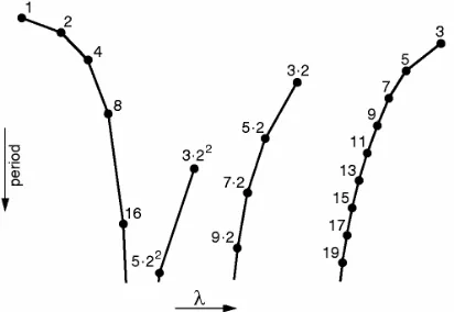
The Sharkovsky theorem gives a clear ordering of the first appearance superstable orbits (see Figure 1), but without taking into account either the symbolic sequence or the origin of each periodic orbit. On the contrary, the outstanding work of MSS [23], which also deals with the issue of ordering, uses both the symbolic sequence and the pattern generation; however, it is difficult to see any ordering there (see Figure 2, where we graphically show the MSS superstable periodic orbit generation according
to the MSS theorem [23]). Figure 1. A sketch of the Sharkovsky theorem for the logis-tic map, xn1xn
1x
20 p
n . First appearance superstable
rbits for periods As said before, PRM harmonics were introduced in
[image:4.595.320.526.410.552.2][12] to better understand the ordering and the generation o are shown.
Figure 2. A sketch of the successive application of the Metropolis, Stein, and Stein theorem in the logistic map
1 1
n n
[image:4.595.72.526.613.704.2]Let us conside al Ma
have repeated is an L-map. As we know from [12,17], a pattern P has even L-parity if it has an even number of Ls, and has odd L-parity otherwise. L-parity is a concept similar to R-parity, introduced by MSS [23] for the logis- tic map, a R-map. Now, the definition of PRM harmonics [12,17] can be seen.
Let P be a pattern. The first PRM harmonic of P, r the re ndelbrot map, which as we
1
PRMH P
changing the even (or
2
PRM, is formed by appending P to itself and second C to L (or R) if the L-parity of P is odd). The second PRM harmonic of P,
H P , is formed by appending P to HPRM 1
P the L-parityand he second C to L (or R) if of changing t
1
PRMH P
As can be
is even (or odd), and so on. seen, in this case the mnem
lero rule (L if Even and R if Odd), which is the canonical
rule for an L-map.
Application: The harmonic structure of 1D quadratic
maps
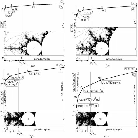
Let us see how to generate the chaotic bands in the real Mandelbrot map by beginning just at the origin, i.e., at the period-1 superstable orbit of symbolic sequence C. For this purpose, we shall be assisted by Figure3, where in the upper parts we depict sketches of the PRM har- monics where periods and symbolic sequences are shown and, in the lower parts, we depict the corresponding Mandelbrot set antenna zones by means of the escape lines method [29]. Obviously, since we are in the 1D case, in these lower parts only the intersection of these figures with the real axis make sense, although we use the whole figure in order to better “see” the periodic or- bits. Let us note that, in the upper parts, symbolic se- quences corresponding to cardioids are only depicted with black half filled circles, while symbolic sequences corresponding to discs are depicted with black circles. In Figure3(a) we show the PRM harmonics of C obtained in accordance with the lero rule. To form the first PRM harmonic of C we add a C to the C, i.e., we write CC and we change the second C into an L, since the L-parity of C is even. Therefore, the first PRM harmonic of C is . To form the second PRM harmonic of to the first one, i.e., we write CLC and we nd C into a R, since the L-parity of CL is ain
the we obtain that the
third and fourth PRM harmonics of C are
and . As is well
], CLR, CLR (CRL, CRL2, bolic se- last appeara orbits. As it
n [12, M har-
ca case the
the preperiod
onic rule is the
1
C CL
PRM
H
C we add a C change the seco odd, and we obt By applying
2
C CLR
PRM
H .
same procedure,
3
2C CLR
PRM
H
known [12,26 CRL3, …, in the l quences of the was already show monics of a pattern limit HPRM
C is 1 and period 1, 1, 4
3C CLR
PRM
H
2
, CLR3, … ogistic map) are the sym
nce superstable 30], the limit of the PR n be calculated. In this Misiurewicz point with
1
M , w nce is (CL)R
(if C account, the preperiod is 2, and we have
hose symbolic seque
is taken into
2,1
M , as can be seen in [12]). This point is the tip (C) [1 whose parameter value is
As seen in the figure, we start from the period-1 su- persta C placed in the pe he first PRM onic of C is the period-2 s ble orbit of the p doubling cascade. All the o armon-
uperstable riod-20
chaotic ba and are the last appea perstable orb is . If we consider th 0 supersta-
gene , then the PR rmonics of
the ge nerate period-20 band
Howe 21 able orbit n th
riod rated. Let hap
when d new gene
Let’ at 3(b) show
harm 2,30],
ble orbit harm eriod ics of C are s
nd its of th ble orbit C as
ne G ver, a ic regio this or
onics of
2 c .
riodic region. T upersta ther PRM h orbits placed in the pe rance su e period-2
M ha chaotic
placed i us see what
1 G . where we 0 B band a ge
is also g bit is use
0 G the superst ene as a Figure 0 n
s now look
0 B . e pe- pens the 1 CL
G . To form its PR onics we add C h one and we cha the second C into ordance with th rule. So, we obtain t at the ond, third, an th PRM har- m
,
, and .
The limit of these harmonics
M harm nge e lero d four CLRL
1 CLH G
is the Misiurewicz point L to t
a L or a R, h onics of
1 PRM 3 PRM e previous in acc first, sec are 1 G
1 CLRLH G , H PRM2
G1 3
51 CLRL
H G 4 7
RL PRM
1 CLR L
[16,17], that separates the and od-21 cha
gene rom CL
whic ponds to t peri ling casca
the M harm
period-21 are t appearan Agai we consider C PRM onics of th chaotic ba B1 (and
now Figure 1 2,
m M
the peri rated f h corres od doub other PR placed in the he last n, if
harm nd Let us see
and fo
2H G
, placed in period-2 otic band is the pattern
he secon de of th onics of C
chaotic b ce supe
L as a gene e gene a new
3(c)
harmonics of the gene e first, second, third, urth harm
89 012
c
0
c band B0
1
B . T t harmonic C period-22, supe orbit of the d n of C. All ar rstable orbits nd in addition, of this band.
G ve that the ge e period-21
2
G ).
ere the PRM
1.543 6 chaoti he firs LRL of rstable ic regio e supe 1
B and, orbits
1, we ha nerate th CLRL we show . Th d e perio L a rstable 1 ne wh G ge 2 CLRL G
onics of G2 are
1 3
CLRL RL
PRM ,
3 2 3 CLRL 2 RL PRM
H G ,
3
3 5 2H G 4
3 7CLRL RL
PRM , and H G2
the periodic region and the the period-2
is the
CLRL RL
PRM ,
the first being a new gene in
others superstable orbits placed in 2 chaotic band . The limit of these harmonics Misiurewicz point
2 B
1
2
2 4,2 CLRL LR
m M
1
[16,17] which separates
chaotic band 2 chaotic
band . Therefore the PRM harm gene
period-22 new gene,
Figure 3(d), show PRM onics of the previous p (23) gene the period-2 2 B generate the CLRL harm 1 B chaotic band , of the next chaotic band.
and the period-2 onics of the
2, and a
ere we eriod-8 2 G the B wh 3 3 RL G
stable orbits of the period doublin cascade i Figure 3. A sketch of the PRM harmonics of the first four sup
e PRM harmonic generation of last appearan chaotic band B0; (b) period-2 chaotic band B1; (c) period-4 ch
3
3 CLRL RL
G . A en
er g n the real
Man-delbrot map. Th ce superstable patterns of c tic bands is shown. (a) Pe -1
aotic band B2; (d) period-8 chaotic band B3.
new period-16 g e in the periodic
ted. The limit
a the M iu
ng cascad
hao riod
reg
of these superst
ion, G4, and the last appearance superstable orbits of the period-23 chaotic band B3 are genera
ble orbits is rewicz point 1
3 8,4
m M [16,17] that separates the period-22 chaotic band B2 and the period-2
3
chaotic band B3.
Generalizing, the PRM harmonics of the gene Gn generate the last appearance superstable orbits of the period-2nchaotic band Bn, and a new gene of the period doubli e, the gene Gn1
is
. Likewise, HPRM
Gn
is a Misiurewicz point mn M2 ,2n n1 [10], a primary
separator (or band-merging point) of the chaotic bands
1 n
B and Bn.
This double procedure (periodic orbits of the period cascade generatio
doubling chaotic band generation)
contin , periodic orbits of the
n and ues i finitely and both
t
].
of th r he set of the
nde
e co
period doubling cascade on he right and chaotic bands on the left, meet in the Myrberg-Feigenbaum point [31
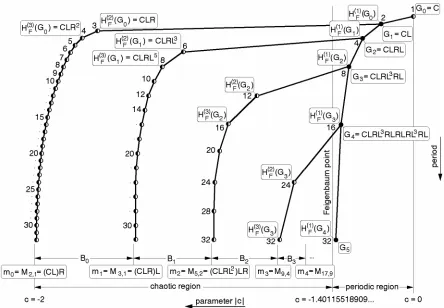
Every pattern of the period doubling cascade is the responding chaotic band. T
gene
PRM harmonics of all the genes is what we call the har-
Figure 4. A sketch of the harmonic structure of the real Mandelbrot map. Each period doubling cascade superstable orbit is a gene Gn. The PRM harmonics of these genes generate the corresponding chaotic band Bn and the Misiurewicz point
that separates the chaotic bands Bn–1 and Bn.
The patterns of the harmonic structure are called struc-
tural patterns and all of them are PRM harmonics. In Figure 4 we can see the periodic region and the chaotic region separated by the Myrberg-Feigenbaum point. Likewise, the chaotic region is divided in an infin- ity of chaotic bands B, separated by Misiurewicz points called separators, mn, . Each structural pattern of each chaotic band and each separator is determined by starting with the only datum of the pattern C, and by ap-
As can be seen in gistic map, a
R--m
t
rightward
ref , we have to
rst P onic of P
, 1
2 2n n
n
m M
n
0 n
plying the successive harmonics to the successive genes, what shows the power as calculation tool of the PRM harmonics.
[image:7.595.77.521.85.393.2]detail in [12], if we deal with the lo- map, instead of with the real Mandelbrot map, a L ap, the result is equivalent to what is shown in Figure 4. However, we have o take into account that in this case, the canonical direction of the logistic map is the direction, the canonical parity is the R-parity and the canonical rule is the relo rule (the ore
interchange Ls and Rs).
To finish this section, we shall see the PRM antihar- monics.
Let P be a pattern. The fi RM antiharm , 1
PRM
A P , is formed by appending P to itself and chang-
ing the second C to R (or L) if the L-parity of P is even (or odd). The second PRM antiharmonic of P, APRM 2
P , is formed by appending P to APRM 1
P-parity of and second C to R (or L) if the L
changing the
1 PRMA P is even
M antihar- never t, although they
nt role in
p, to obtain (or odd). And so on.
As in the case of MSS an monics are also a purely correspond to a periodic orbi have no real existence, the
ics. e ith the lo an
th
tiharm form
t either. B y play an
gistic map, a R onics, PR al construction and
u importa
-ma
some cases, as we shall see later. However, in the case of the structural patterns that we have treated here only PRM harmonics are present.
We are dealing with the real Mandelbrot map, a L-map, and we have to apply the relo rule to obtain antiharmon-
If we w re w
tiharmonics we would have to apply the lero rule; that is, just the opposite than in the case of harmonics.
obtained by applying the anticanonical rules, and they grow in the anticanonical direction.
3. Harmonics in 2D Quadratic Maps
In the same way as in Section 2 we reviewed harmonics (both MSS harmonics and PRM harmonics) in 1D quad- ratic maps, in this section we review both types of har- monics in 2D quadratic maps. The main difference be- tween both cases is that the identifiers are the symbolic sequences for the 1D case, and the EAs (which we only use here in the binary expansion form) for the 2D case.
However, in both cases, the MSS harmonics calculate the identifiers of the period doubling cascade, placed in the periodic region, and the PRM harmonics calculate the identifiers of the last appearance HCs (LAHCs), placed in the chaotic region. As said before, the 2D quadratic map used here is the Mandelbrot set, which can be seen in Figure 5(a). Let us see next MSS harmonics in Sec- tion 3.1 and PRM harmonics in Section 3.2.
3.1. MSS Harmonics
For the 2D case, when we start from a period-p HC and we progress through its period doubling cascade, we find discs whose periods are 21·p, 22·p, 23·p, ... In the same way as MSS introduced the concept of harmonics in 1D
y itself an bviously we
unimodal maps [23], by extension we call MSS harmon- ics of a HC of the Mandelbrot set to the set constituted b d all the discs of its period-doubling cascade
refer to their identifier). (o
Let
. , .a a1 2
be the two EAs of a HC. By taking into account that the EAs of the period-2 disc are
.01, .10
(see Figure 5(a)), it is easy to obtain the EAs of a MSS harmonic of
. , .a a1 2
from the tuning algorithm of Douady and Hubbard [21,32]. Therefore, we can define the MSS harmonics as follows:Let
. , .a a1 2
be the two EAs of a HC. The succes- sive MSS harmonics of the HC are given by: 0
1 2 1 2
. , . . , .
MSS
H a a a a , HMSS 1
. , .a a1 2
.a a a a1 2, . 2 1
, 2
1 2 1 2 2 1 2 1 1 2
. , . . , .
MSS
H a a a a a a a a a a
,
3
1 2 1 2 2 1 2 1 1 2 2 1 1 2 1 2 2 1
. , . . , .
MSS
H a a a a a a a a a a a a a a a a a a , …
1 2 . , . MSS
H a a are the EAs of the Myrberg-Feigenbaum point. This notable point has neither binary nor rational EAs.
Example 1
The EAs of the Mandelbrot set main cardioid are
.0, .1of the s
. By applying the previous expressions, the EAs uccessive discs of the period doubling cascade of such a main cardioid can be calculated. The first MSS harmonics, up to the fourth, are:
0
.0, .1 .0, .1 MSSH , H MSS1
.0, .1 .01, .10
, 2
.0, .1 .0110, .1001
MSS
H ,
3
.0, .1 .01101001, .10010110
MSS
H and
4
.0, .1 .0110100110010110, .1001011001101001
MSS
H ,
as can be seen in Figure 5(a).
Example 2
If we start from the cardioid of any other midget, we can also calculate the EAs of the discs of its period dou- bling cascade. Look at Figure 5 where Figure 5(a) shows the Mandelbrot set; Figure 5(b) shows a sketch of the shrub (1 3) marked with the rectangle c in Figure 5(a); and Figure 5(c) shows the shrub (1 3) that is a magnify- cation of the mentioned rectangle c. Let
.00111, .01000
be the EAs of the period-5 cardioid placed in the branch 11 of the shrub (1 3) [33] (see firstly Figures 5(b) and 5(c)). Figure 6(a) shows a magnification of the branch 11 where this period-5 representative can be better observed, and Figure 6(b) shows an additional ma n of such a period-5 representative. The
gnificatio
EAs of the successive discs of the period doubling cascade of such a period-5 cardioid can be calculated. Calculating the MSS harmonics, up to the third, we obtain:
0
.00111, .01000 .00111, .01000
MSS
H , HMSS 1
.00111, .01000
.0011101000, .0100000111
, 2
.00111, .01000 .00111010000100
MSS
H
000111, .01000001110011101000 ,
3 .0011101000010
.00111, .01000
.010000011100111 MSS
H
as can be seen in Figure 6(b).
Antiharmonics of MSS seem again to have no interest, as we can deduce next from th
000
eir definition:
011101000001110011101000,
0100000111010000100000111 ,…,
Let
. , .a a1 2
be the two EAs of a HC. The success- sive MSS antiharmonics of the HC are given by: 0
. , .1 2 . , .1 2
MSS
A a a a a , 1
. , .
. , .
2
1 2 1 1 1 1 2 2 2 2
. , . . , .
MSS
A a a a a a a a a a a ,…
Therefore, all of them are the same, which is the start-ing HC.
3.2. PRM Harmonics
1 2 1 1 2 2
MSS
Figure 5. (a) Mandelbrot set with the first four external argu rnal a s. Shrub (1/3) is framed in rectangle c. (b) Sk in (a). (c) Shrub (1/3) that is a magnification of the rec
ments of the period doubling cascade, and other significant
ex-te rgument etch o
tangle c mark
[image:9.595.79.513.83.697.2]Figure 6. (a) Magnification of the branch 11 of the shrub (1/3) shown in Figures 5 (b) and (c), where the period-5 representa-tive can be better observed. (b) Magnification of such a period-5 representarepresenta-tive shown in the rectangle b marked in (a), with some of its important external arguments.
Let
. , .a a1 2
expansionbe the EAs of a HC given in form of binary [22]. The EAs of the order i PRM har- monics of
. , .a a1 2
are given by:
1 2 1 2 2 2 2 1 1 1
. , . . , . .
i PRM
i i
H a a a a a a a a a a
(1)
When , Equation (1) calculates a
se-quence o Equation (1) becomes:
0, 1, 2, 3,
i
f HCs. When i ,
1 2 1 2 2 2 2 1 1 1 1 2 2 1
. , . . , . . ,.
PRM
H a a a a a a a a a a a a a a
(2) two preperiodic arguments, and therefore Misiurewicz points.
In the 1D case, we obtained the harmonic structure through repeated application of the PRM harmonics.
Similarly, in the 2D case Equation (1), applied to a given HC when i0, 1, 2, 3,
f inal HC. Indeed
). By applying Eq M harmonics of G
se that normally n
, calculates a sequence of HCs which are the LAHCs o the corresponding chaotic band of the orig , let us analyze, as an ex-ample, the main cardioid that we consider as a gene (see Figure 7 uation (1) we obtain
successive PR . For we ob
, a trivial ca t will en into
count, for
0
G
the tain ac-0
o
0
i
be tak 0
G
1
i we obtain 2
i we o
0. If we apply n isiurewicz point
a new gene b o
1
G in e w Equation (
the
regi tain th LAHCs of
chaotic band 2) to
ain t
the
0
G , odic
we obt
on, and for
B
he M M1,1, which
is, is th
xtrem
[image:10.595.137.460.80.503.2]Figure 7. The neighbourhood of the main antenna of the Mandelbrot set with three chaotic bands, B0, B1 and B2, showing the
EAs of their first LAHCs. Likewise, the main cardioid G0 and the discs of the period doubling cascade, G1, G2, ···, showing
their EAs.
considered the gene or generator of the chaotic band Likewise, by applying now Equation (1) to the new
, we obtain, after the trivial case of , first a new in the periodic region, and t LAHCs o
nd . If we apply now tion (2 ain th siurewicz point
0 B . gene f ) to 1 G gene 1 G 0 i hen the Equa 2,1 2 G
the chaotic ba , we obt
1
B
e Mi M , wh
. That is, th 1) to ew gen
ich e chaotic band
ered th gene or generato e chaot . In neral, b ying Equat a
, after th ial case, first a n e
is the can band n G 1 upper extrem consid ge tain of the e y appl e triv 1 r of on ( B i 1 G ic gene n G be 1 B
we ob in
ob-ppe be n B . oni r c th band tain extre consi
e peri c regi d then . If we a now Equa
isiur oint
the ge Wh we ha st seen
structure of the 1D case. However, since now we are in the 2D case, we only calculate the structure of the chaotic bands of the cardioid considered. Let us see two exam- ples, the first one applied to the main cardioid (see Fig- ure 7), and the second one to the period-5 midget of the branch 11 of the shrub
odi n B the M m dered at on, an pply ewicz p e of the chaotic band
gene or ve ju
the LAHCs of the chaotic to
ich . That is,
e chaotic lar to the h tion (2) 1 h i n G is th n G , we e u can arm 2 ,2n n
M
n
B
nerator of t is sim
, wh
band
(1 3 ) in the chaotic region (see Figure 6(b)).
Example 1
In Figure 7 we can see the neighbourhood of the main antenna of the Mandelbrot set with three chaotic bands, and , and also the main cardioid and scs of period doubling cascade, ….
of t od-1 main cardioid, the g , are 0 B , the d The E 1 B i As 2 B the he peri 0 G
, G2
0 G 1 G ene ,
0 .0, . 1
G . If Equation (1) is applied to this main
car-dioid, H PRMi
.0, . 1
, for i0, 1, 2, 3,, the sequence
.0, . 1
,
.01, .10
,
.011, .100
,
.0111, .1000
,
.01111, .10000
,…is obtained. The values of this sequence (without taken into account the first one) are: first the gene , and then the LAHCs of the chaotic band . If no ap- ply Equation (2), we obtain
1 G w we 0 B
.0, . 1 .0 1,.10
PRM
H , a
Misiurewicz point, m0M1,1, which is the upper ex- treme of B0. Likewise, let us consider now
1
.01, .10 .01, .10 PRMH as a new gene G1
.01, .10
.By applying Equation (1) to G1,
.01, .10 iPRM
H for
0, 1, 2, 3,
i , we obtain the sequence
.01, .10
,
.0110, .1001
,
.011010, .100101
,
.01101010, .10010101
,
1010, .1001010101
,…which corresponds to (after the obvious ) first the gene , and then the LAHCs of the ch band If no apply Equation (2) we obtain
.011010 , 1 G aotic 2 G w we 1 B .
.01, .10 .0110,.1001 PRM
H , a Misiurewicz point,
,1
1 2
m M , which is the upper extreme of B. Finally, we can consider
1
1
.01, .10 .0110, .1001 PRM
H as a new
gene G2
.0110, .1001
. By applying Equation (1) to2
.0110, .1001
,
.01101001, .10010110
,
.011010011001, .100101100110
,
.0110100110011001, .1001011001100110
,
.01101001100110011001, .10010110011001100110 ….
After , these terms are first the gene and then th of the chaotic band . By ap ing Equa-tion (2 ain2
G
e LAHCs ) we obt
3
G , ply 2
B
.0110, .1001 .01101001,.10010110 PRM
H ,
a Misiurewicz point, ,2, which is the upper ex- treme of B2. And so ch that, in a general case, Gn generates the chaotic band Bn (not shown in the figure).
Example 2
Let us see the period-5 midget of the branch 11 of the shrub(
2 4
m M
on, su
1 3) th
shown in Figure 6(b) which is a magnifica- tion of e rectangle b shown in Figure 6(a). Let us con- sider this period-5 cardioid as a gene whose EAs are
0 .00111, .01000
G .
If we apply Equation (1),
0 .00111, .01000
i i
PRM PRM
H G H , for
we obtain the sequence
0, 1, 2, 3,
i ,
.00111, .01000
,
.0011101000, .0100000111
,
.001110100001000, .010000011100111
,
.00111010000100001000, .01000001110011100111
,…, whose terms (for ) are the LAHCs of the chaotic band . If now y Equation (2),2
i
we appl 0
B
.00111, .01000 .0011101000,.0100000111 PRM
H ,
a Misiurewicz point, m0M5,5, which is both the tip of e dget and the upper e
void prob gure.
Antiharmonics of PRM neither seem to have any in- terest, as in previous cases. Indeed, according t definition:
th mi xtreme of B0. As always, we can do the same procedure in order to calculate the LAHCs of the rest of the chaotic bands. We have not done it to a lems with the fi
o their
Let
. , .a a1 2
be th he Ee EAs of a HC given in form of binary expansions [22]. T As of the order i PRM an- tiharmonics of
. , .a a1 2
are given by:
1 2 1 1 1 1 2 2 2 2 1 2
. , . . , . . , .
i PRM
i i
A a a a a a a a a a a a a
Equation (3) becomes:
(3)
When i ,
1 2 1 1 1 1 2 2 2 2 1 2
. , . . , . . , .
A a a a a a a a a a a a a
(4)
The result in both equations is the starting HC. However, these concepts will be very useful in the next section.
4. Pseudoharmonics and
Pseudoantiharmonics in the 2D Case
We have just seen that the PRM harmonics are a power- ful tool for calculating some EAs in 2D quadratic maps. However, we can go much further if we introduce an extension of these calculation tools, which we simply call pseudoharmonics and pseudoantiharmonics [35]. These new tools are applied to the EAs of two HCs, as we can see next.
4.1. Introduction of Pseudoharmonics and Pseudoantiharmonics
The introduction of pseudoharmonics and pseudoanti- harmonics can be seen in detail in [35]. Let us first in- troduce pseudoharmonics. Let
. , .a a1 2
be the externalarguments of a HC, and let
. , .b b1 2
be the externalarguments of other HC that is related with the first one, as will be seen later. The external arguments of the order
i pseudoharmonics of
. , .a a1 2
and
. , .b b1 2
are:
1 2 1 2 1 2 2 2 2 1 1 1
. , . ; . , . . , .
i
i i
PH a a b b a b b b a b b b
(5) When i0, 1, 2, 3,
of HCs that we
, Equation (5) calculates a se- quence shall determin afterwards. When e
i , Equation (5) becomes:
.a b a b, .
1 2 1 2 1 2 2 2 2 1 1 1
. , . ; . , . . , .
PH a a b b a b bb a b bb
1 2 2 1
(6) Equation (6) calculates a pair of external arguments of a Misiurewicz point. Later we shall analyze this result in every possible case.
Let us now introduce pseudoantiharmonics. Let
. , .a a1 2
be the external argu ents of a C, and let m H
. , .b b1 2
b e external arguments of ther HC, that is related with the first one. The external arguments of the order i pseudoantiharm cs ofe th o
oni
. , .a a1 2
and
. , .b b1 2
1 2 1 2 1 1 1 1 2 2 2 2
. , . ; . , . . , .
i
i i
PA a a b b a b b b a b b b
(7) When , Equation (7) calculates a se- quence and not the starting HC as in the case of Equatio e, although PRM antiharmonics seemed t ey have been useful in order to
introdu onics. When , Equation
(7) becomes: 0, 1, 2, 3,
i
of HCs, n (3). Therefor
o be of no use, th
ce pseudoantiharm i
1 2 1 2 1 1 1 1 2 2 2 2
1 1 2 2
. , . ; . , . . , .
. , .
PA a a b b a b b b a b b b
a b a b
(8) Equation (8) calculates a pair of EAs of a Misiurewicz point, and not the starting HC as in the case of Equation
late more EAs.
n e, h
av
(4). Again PRM antiharmonics are suitable to introduce pseudoantiharmonics that, as we shall see, are very use-
l to calcu fu
Pseudoharmonics and pseudoantiharmonics are, as has been said, a generalization of PRM harmonics and PRM a tiharmonics in the 2D case; therefor t ese two last ones h e to be a particular case of the two first ones. In- deed, when
. , .b b1 2
. , .a a1 2
, Equations (5), (6), (7) and(8) become Equations (1), (2), (3) an (4). Thus, in this case, pseudoharmonics and pseudoantiharmonics have become PRM harmonics and PRM antiharmonics. Let us see it from other approach. Pseudoharmonics and pseu-doantiharmonics are applied to two HCs whereas PRM harmonics and PRM antiharmonics are applied to only one HC. However, PRM harmonics and PRM antihar-monics can be thought as pseud harantihar-monics and pseudo-antiharmonics where their two HCs are the same.
d
o
4.2. Some Considerations to Calculate
Pseudoharmonics and Pseudoantiharmonics
To apply what we have seen so far, we shall briefly re- member some concepts that can be seen in detail in [35].
We call a descendant [35] of
. , .a a1 2
and
. , .b b1 2
to any of the HCs obtained from Equations (5) and (7). Li zone occupied by all the descendants cal- cu
firs air kewise, the
lated by using these equations is the zone of descen-
dants [35]. In other to calculate a descendant, given the t p ,
. , .a a1 2
, the second pair cannot be any
, .b2
.Indeed,
1 .b
. , .b b1 2
has to be an ancestor [35] of
. ,a a1 . 2
. Let us briefly see the ancestors of
. , .a a
, which willbe used ation o onics and pseu-
1 2
in the calcul f pseudoharm
doantiharmonics (descendants). The second pair
. , .b b1 2
is an ancestor of the first pair
. , .a a1 2
if
. , .a a1 2
is a descendant of
. , .b b1 2
and
. , .c c1 2
, where
. , .c c1 2
itself is an ancestor of
. , .b b1 2
. Notethat any HC is an ancestor of itself. Note also that the ancestor of a HC has lesser or equal period than the pe- riod of such a HC. In order to determine the ancestors of
. , .a a1 2
, next we shall remember some points.As known from [33,36], the shrub of the n-ary hyper-
bolic component 1 1 1 1 N N q q p p
, shrub( 1 1 1 1 N N q q p p
), has n
subshrubs or chaotic bands, S1SN gene or
, each one of them generated by one HC called generator [33,35,36] of the chaotic band or subshrub. The generator of the last
subshrub, SN, is the main cardioid 11, that is e first
component of the generation route of
th 1 1 1 1 N N q q
. The
p p
generator of the last but one su ub, , is the pri-
mary disc
bshr SN1
1 1
1 1
q
, that is the second component of the
p
generation route of 1 1 1 1 N N q q p p
. Likewise, the generator
of SN2, is the secondary disc 1 2 1 2
1 q q
1p p , that is the
third component of the generation route of 1 1
1 1 N N q q , p p
and so on. Finally, the generator of the first subshrub, S1,
is the (N-1)-ary disc 1 1
1 1
1 1
N
p p
, om-
eneration ro e of
N
q
q
that is the Nth c
ponent of the g ut 1 1 N
1
1 N
q
p p . Hence, in general, the generator of the subshrub is the (N-i)-
ary disc q i S 1 1 1 1 N i N i q q p p
, that is the (N-i+1)th component
of the generation route of 1 1 1 1 N N q q p p .
Let
. , .a a1 2
be the representative of a branch (whosebranch associated number is .
The first ancestor of
1 2 m
d d d [33]) of Si
. , .a a1 2
is the generator 11
1
1 N i
N i
p p
q
q
Si where
the br found. The second, third, … of the chaotic band or subshrub
anch is
ancestors of
1 2 m
d d d
. , .a a1 2
are:1 1 1 1 1 N i
1 N i
q ,
q p p 2 1 1 1 N i q q
p1 pN i 2
in the generation route of
1 1 1 1 N N q q p p
, up to 1 1
1 1 1 1 N N q q p p
and 1
1 1 1 N N q q
p p , all of them in the periodic region. T lowing ancestors
of
he fol
. , .a a1 2
, now in the chaotic region, he repre- sentatives of the branches …,can be seen, all the ancestors o e in
th bs
are t
. As 1
d , d d1 2, of the cha
1 2 m
d d d tic region ar
Si, and ere is no one in the other subshru . What we call ancestor route includes all the ordered ancestors of
. , .a a1 2
from the generator 1 1 1 1 N i N i q q p p to
1 1 1 1 N N q q p p
in the pe ion, followed by the rep-
resentatives of the branches d1, d d1 2,…, d d1 2dm in
th ion.
riodic reg
on e chaotic reg
4.3. Z es of Descendants
As can be seen in detail in [35], depending on the ances- tor
. , .b b1 2
we shall have a different zone of descen- dants. Let us see the most important cas . es1st case:
. , .b b1 2
is the first ancestorIf
. , .a a1 2
is the representative ch of , the first ancestor ofof the bran
1 2 m i
d d d S
. , .a a1 2
,
. , .b b1 2
, is the generator 1 1 1 1 N i N i q q p p of 5]. In
this case,
i S [3
1 2 1 2
. , . ; . , . i
PH a a b b
ca the rep-resentatives of the branches hat i
an nd so on. Ob-
viously, wh
lculates
. T
1 2 m1 1 i
d d d s to
say, it successively calculates first the representative of the branch d d1 2dm, and then the representatives of the br ches d d1 2dm1, d d1 2dm11, a
en i one has:
1 1 2 2 1
. , . . , .
PH a a a b a b
that is the pair of external arguments the Misiurewicz point placed in the upper extreme of the branches
1 2 m11
d d d . Therefore,
2 ; . , .b b1 2
of
. , .
; . , .
.PH a a1 2 b b1 2 a b1 2, .a b2 1
calculates the upper extreme of the zone of descendants of
. , .a a1 2
and
1 2
. , .b b , and
. , .1 2
; . , .1 2
i
PH a a b b calculates de LAHCs in that
zone. The zone of descendants finishes in a tip or upper extreme of ; therefore, this zone of descendants cov-ers the wh ubshrub
2nd case: i S
ole s Si.
. , .b b1 2
is the second ancestor, 11
1 1
1
. , .a a1 2
be the representative of a branch of . Since the first ancestor is1 N i
N i
p p
q
q
Let
1 2 m
d d d Si
1 1 1 1 N i N i q q p p
, that is the generator of Si, the second
ancestor is 1 1
1 1 1 N i 1 N i p p q
q
. Let
. , .b b1 2
be the externalarguments of this second ancestor. Then
1 2 1 2
. , . ; . , .
PH a a b b and
1 2 1 2
. , . ; . , .
PA a a b b
respectively calculate the upper and lower extremes of
the zone of descendants of
. , .a a1 2
and
. , .b b1 2
. And,in this case, the zone of descendants is the branch
1 2 m
d d d . On the other hand,
1 2
. , . ; . , . i
PH a a b b1 2 and
1 2 1 2
. , . ; . , . i
PA a a b b , i0, 1, 2, 3,,
respectively calculate the LAHCs i increasing and decreasing directions of the bran d .
3rd case:
n the ch d d1 2 m
. , .b b1 2
is the third, fourth, …, ancestor (except for the last one).Let
. , .a a1 2
be the representative of a branch1 2 m
d d d of Si. Its ancestors in the periodic region are:
1 1 1 1 N i N i q
q 1 1
1 1 1 1 N i N i q q p p p p , , 2 1 1 2 1 1 N i N i q q
p p
, …, 1
1 1 1 N N q q p p ,
an cestors in the c
fore, t
d its an haotic region are the representa- tives of the branches d1, d d1 2, …, d d1 2dm. There-
he third ancestor is 1q1 2
1 2 1 N i N i q p p
if we are still
in the periodic region, and the representative of the branch d1 if we are not. Now,
1 2 1 2
. , . ; . , .
PH a a b b
and
. , .1 2
; . , .1 2
PA a a b b
respectively calculate the upper and lower extremes of the zone of descendants of
. , .a a1 2
and
. , .b b1 2
, thatin her
hand,
this case is a sub-branche of d d1 2dm. On the ot
1 2 1 2
. , . ; . , .
PHi a a b b
and
1 2 1 2
. , . ; . , . i
PA a a b b , i0, 1, 2, 3,,
respectively calculate the LAHC decre