Original citation:
Yu, A. C. (2004) Efficient intra- and inter-mode selection algorithms for H.264/AVC. University of Warwick. Department of Computer Science. (Department of Computer Science Research Report). CS-RR-404
Permanent WRAP url:
http://wrap.warwick.ac.uk/61319
Copyright and reuse:
The Warwick Research Archive Portal (WRAP) makes this work by researchers of the University of Warwick available open access under the following conditions. Copyright © and all moral rights to the version of the paper presented here belong to the individual author(s) and/or other copyright owners. To the extent reasonable and practicable the material made available in WRAP has been checked for eligibility before being made available.
Copies of full items can be used for personal research or study, educational, or not-for-profit purposes without prior permission or charge. Provided that the authors, title and full bibliographic details are credited, a hyperlink and/or URL is given for the original metadata page and the content is not changed in any way.
A note on versions:
The version presented in WRAP is the published version or, version of record, and may be cited as it appears here.For more information, please contact the WRAP Team at:
Annual Report
EFFICIENT INTRA- AND INTER-MODE SELECTION
ALGORITHMS FOR H.264/AVC
Andy C. Yu
Department of Computer Science
University of Warwick, Coventry CV4 7AL, UK
EFFICIENT INTRA- AND INTER-MODE SELECTION
ALGORITHMS FOR H.264/AVC
by
Andy C. Yu
ABSTRACT
H.264/AVC standard is one of the most popular video formats for the next generation video coding. It provides a better performance in compression capability and visual quality compared to any existing video coding standards. Intra-frame mode selection and inter-frame mode selection are new features introduced in the H.264/ AVC standard. Intra-frame mode selection dramatically reduces spatial redundancy in I-frames, while inter-frame mode selection significantly affects the output quality of P-/B-frames by selecting an optimal block size with motion vector(s) or a mode for each macroblock. Unfortunately, this feature requires a myriad amount of encoding time especially when a brute force full-search method is utilised.
In this report, we propose fast mode-selection algorithms tailored for both intra-frames and inter-intra-frames. The proposed fast intra-frame mode algorithm is achieved by reducing the computational complexity of the Lagrangian rate-distortion optimisation evaluation. Two proposed fast inter-frame mode algorithms incorporate several robust and reliable predictive factors, including intrinsic complexity of the macroblock, mode knowledge from the previous frame(s), temporal similarity detection and the detection of different moving features within a macroblock, to effectively reduce the number of search operations. Complete and extensive simulations are provided respectively in these two chapters to demonstrate the performances.
Finally, we combine our contributions to form two novel fast mode algorithms for H.264/AVC video coding. The simulations on different classes of test sequences demonstrate a speed up in encoding time of up to 86% compared with the H.264/AVC benchmark. This is achieved without any significant degradation in picture quality and compression ratio.
TABLE OF CONTENT
Title page i
Abstract ii
Table of content iii
List of figures v
List of tables vii
Glossary viii
Chapter 0 Video basics 1
0.1 Colour component 1
0.2 Video format 2
0.3 The structure of a video sequence 2
0.4 Motion estimation and compensation 3
0.5 Transform coding 3
0.6 Quantisation 4
0.7 Visual quality evaluation 5
0.8 Intra-coding and inter-coding 5
Chapter 1 Overview of texture coding in H.264/ AVC 6
1.1 Introduction 6
1.2 Lagrangian rate-distortion optimisation 7
1.3 Contribution and organisation of this report 10
Chapter 2 Proposed intra-frame mode selection algorithm 11
2.1 Introduction 11
2.2 Algorithm formulation 12
2.3 The proposed fast algorithm 16
Chapter 3 Proposed inter-frame mode selection algorithms 20
3.1 Introduction 20
3.2 Algorithm formulation 20
3.3 The proposed inter1algorithm 23
3.4 The proposed inter2algorithm 26
3.5 Simulation results 31
Chapter 4 Comparison results of the combined algorithms 32
Chapter 5 Conclusions and the prospect 36
5.1 Main contributions 36
5.2 Timetable for the research projects (the past 36
and the prospect)
5.3 Future prospects 37
5.4 List of publications 41
LIST OF FIGURES
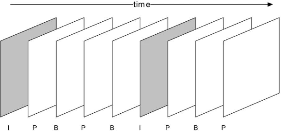
Fig. 0-1 Illustration of the three frame types (I-, P-, and B-).
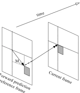
Fig 0-2 Motion compensated prediction and reconstruction.
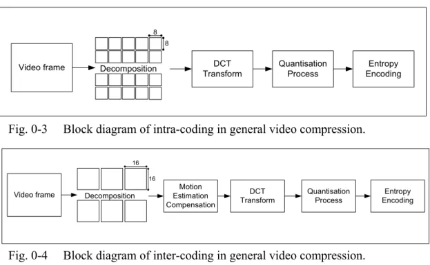
Fig. 0-3 Block diagram of intra-coding in general video compression
Fig. 0-4 Block diagram of inter-coding in general video compression
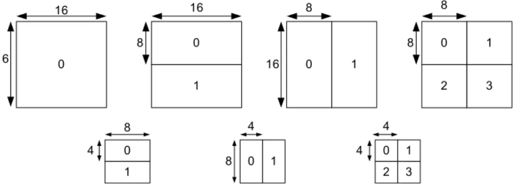
Fig. 1-1 INTER modes with 7 different block sizes ranging from 4×4 to 16×16.
Fig. 1-2 A 4×4 block with elements (a to p) which are predicted by its neighbouring
pixels.
Fig. 1-3 Eight direction-biased I4MB members except DC member which is directionless.
Fig. 2-1 Match percentage between the least distortion cost acquired from SAD implementation and the least rate-distortion cost obtained from Lagrangian evaluation.
Fig. 3-1 The proposed scanning order of En and Sn, the energy and sum of intensities in 4×4 block in order to reduce computational redundancy.
Fig. 3-2 The flowchart diagram of the proposed Finter1 algorithm incorporates the complexity measurement for a macroblock.
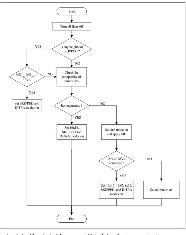
Fig. 3-4 Flowchart of the proposed Finter2 algorithm incorporating the complexity measurement for a macroblock, temporal similarity, and the detection of different moving features within a macroblock.
Fig. 4-1 Snapshot frames of the less common sequences used: (top left to right) City (Class B); Crew and Harbour (Class C); (bottom left to right) Paris (Class B); Template and Waterfall (Class C).
LIST OF TABLES
TABLE 2-1 Simulation results of the proposed Fintra algorithm compared with JM6.1e, the H.264/AVC software, in three sequence classes and two resolutions.
TABLE 3-1 The relationship between the three categories in the proposed algorithm and the 9 members of inter-framemodes.
TABLE 3-2 Simulation results of the proposed Finter1 and Finter2 algorithms compared withJM6.1e, the H.264/AVC software, in three sequence classes.
TABLE 4-1 Simulation results of the two proposed combined algorithms, namely, Fintra + Finter1 and Fintra + Finter2, versus the JM6.1e, H.264/AVC software, for three sequence classes and two resolutions.
TABLE 5-1 The table specifies the important events and the dates October 2003 to June 2004.
TABLE 5-2 The table describes the Core Experiments of MPEG SVC proposed by
JVT.
Glossary
4:2:0 (sampling) A colour sampling method. Chrominance components have
only half resolution as luminance component (see Chapter 0).
AC Alternative Current, refer to high frequency components.
ASVC Advance Scalable Video Coding (see Chapter 5)
Arithmetic coding A lossless coding method to reduce redundancy.
AVC Advanced Video Coding (see Chapter 1)
Block A region of a macroblock, normally 8x8 or 4x4 pixels.
Block matching Motion estimation carried out on block-based.
CABAC Context-based Adaptive Binary Arithmetic Coding.
CAVLC Context-based Variable Length Coding.
CE Core Experiment (see Chapter 5)
Chrominance Colour space (see Chapter 0).
CIF Common Intermediate Format (see Chapter 0).
CODEC Coder / DECoder pair.
DC Direct Current, refer to low frequency components.
Entropy coding A coding method make use of entropy (information of data), including Arithmetic coding and Huffman coding.
Finter1 Fast inter mode selection algorithm 1 (see Chapter 3).
Finter2 Fast inter mode selection algorithm 2 (see Chapter 3).
Fintra Fast intra mode selection algorithm (see Chapter 2).
Full search A motion estimation algorithm.
GOP Group of Picture (see Chapter 0).
H.261 A video coding standard.
H.263 A video coding standard.
H.264/AVC A video coding standard (see Chapter 1).
Huffman coding An entropy coding method to reduce redundancy.
Inter (coding) Coding of video frames using temporal block matching (see
Chapter 0).
Intra (coding) Coding of video frames without reference to any other frame
(see Chapter 0).
I-picture/frame Picture coded without reference to any other frame.
ISO International Standard Organisation, a standards body.
JVT Joint Video Team, collaboration team between ISO/IEC MPEG and ITU-T VCEG.
Macroblock A basic building block of a frame/picture (see Chapter 0).
Motion Reconstruction of a video frame according to motion estimation
compensation of references (see Chapter 0).
Motion Prediction of relative motion between two or more video
estimation frames (see Chapter 0).
Motion vector A vector indicates a displaced block or region to be used for
motion compensation.
MPEG Motion Picture Experts Group, a committee of ISO/IEC.
MPEG-1 A multimedia coding standard.
MPEG-2 A multimedia coding standard.
MPEG-4 A multimedia coding standard.
Objective quality Visual quality measured by algorithm (see Chapter 0).
Picture/frame Coded video frame.
P-picture/frame coded picture/frame using motion-compensated prediction from one reference frame.
PSNR Peak Signal to noise Ratio (see Chapter 0).
Quantise Reduce the precision of a scalar of vector quantity (see Chapter 0).
RGB Red/Green/Blue colour space (see Chapter 0).
SAD Sum of Absolute Difference.
SVC Scalable Video Coding.
Texture Image or residual data.
VCEG Video Coding Expert Group, a committee of ITU.
VLC Variable Length Code.
YCbCr Luminance, Blue chrominance, Red chrominance colour space
(see Chapter 0).
Chapter 0
Video Basics
This chapter aims at defining several fundamentals on video basics and video compression. Those characteristics will help us to understand how video compression works without actually introducing perceptual distortion.
0.1 Colour components
Basically, three primary colour signals, red, green and blue signals (RGB-signal) are generated during the scanning of a video camera. However, the RGB-signal is not efficient for transmission and storage purposed because it occupies three times the capacity as a grey-scale signal. Due to high correlation among the three colour signals and compatibility with the grey-scale signal, NTSC, PAL, and SECAM standards [25] are generated to define the colour in different implementations. Among these, the PAL standard is widely used in video coding research to represent a colour video signal. It has three basic colour representations, YUV, where Y represents the luminance and U (or Cr) and V (or Cb) represent the two colour components. The conversion equations
between RGB and YUV can be represented as
B 114 . 0 G 587 . 0 R 299 . 0
Y= + +
) Y B ( 492 . 0
U= −
) Y R ( 877 . 0
V= −
0.2 Video format
per frame. The corresponding two chrominance (Cr and Cb) components have the
same vertical resolution as luminance, but horizontal resolution is one-quarter. Such a combination of Y, U and V components is called the 4:2:0 sampling format. QCIF format, like the CIF format, makes use of the 4:2:0 sampling format but only one-quarter the size of CIF format.
0.3 The structure of a video sequence
A video sequence can be described as many groups of pictures (GOP) with three different types, Intra-coded (I-), Predictive (P-), and Bidirectional-predictive (B-) pictures/frames, Fig. 0-1. I-frames, the first frames in GOPs, are coded independently without any reference to other frames, whereas P- and B- frames are compressed by coding the differences between the picture and reference(s), either I- or other P-frames, thereby exploiting the redundancy from one frame to another.
Each frame of a video sequence is decomposed into smaller basic building blocks called macroblocks. A macroblock consists of a 16x16 sample array of luminance (Y) sample together with one 8x8 block of sample for each of two chrominance (Cr and
Cb) components.
0.4 Motion Estimation and Compensation
Block-based motion estimation and compensation are used to exploit the temporal redundancies between the encoding frame and reference frame(s), Fig. 0-2. Motion compensation is a process of compensating for the displacement of moving objects
tim e
I P B P B I P B P
from one frame to another. In practice, motion compensation is preceded by motion estimation, the process of finding a corresponding best matched block. In general, we segment the current frame into non-overlapping 16×16 pixel macroblocks, and for each macroblock, we determine a corresponding 16×16 pixel region in the reference frame. Using the corresponding 16×16 pixel region from the reference frame, the temporal redundancy reduction processor generates a representation for the current frame that contains only the changes between the two frames. If the two frames have a high degree of temporal redundancy, then the difference frame would have a large number of pixels that have values close to zero.
0.5 Transform coding
The function of block-based transform coding is to achieve energy compaction and separate the low spatial frequency information from high spatial frequencies. The discrete cosine transform is one of the most popular transformation methods utilised in video coding. The N×N two-dimensional DCT is defined as:
∑∑
− = − = + + = 1 0 1 0 2 ) 1 2 ( cos 2 ) 1 2 ( cos ) , ( ) , ( 2 ) , ( N x N y N v y N u x y x f v u C N v uF π π
Forw ard p
rediction refere
nce frame
Current fra me
Mv
time
= = otherwise , 1 0 , for , 2 1 ) ,
(u v u v
C
where x, y are coordinates in the spatial domain, and u, v are coordinates in the frequency domain.
0.6 Quantisation
Quantisation is an irreversible process to represent the coefficients for high spatial frequencies with less precision. That is because human perception is less sensitive to high spatial frequencies. A DCT coefficient is quantised/divided by a nonzero positive integer called a quantization value, quv, and the quotient, rounded to the nearest integer. The process of quantization, Q(F(u,v)), is expressed as
= uv q v u F v u F
Q( ( , )) round ( , )
0.7 Visual quality evaluation
The most recognised objective measurement of visual quality is peak-to-peak signal-to-noise ratio (PSNR) [26]. It is defined as:
(
)
− × × =∑∑
M i N j j i j i N M 2 ori rec 10 ) , ( Y ) , ( Y 1 255 255 10log PSNRwhere Yrec(i,j) and Yori(i,j) are the luminance values of the reconstructed and original
video signals respectively, and M and N are the number of pixels in the horizontal and vertical directions.
0.8 Intra-coding and inter-coding
The working diagrams of the intra-coding and inter-coding processes are depicted in Fig. 0-3 and Fig. 0-4, respectively. These two block diagrams are similar to each other in terms of the DCT transformation, quantisation process, and entropy encoding. The difference is that the inter-frame encoder decomposes a video frame into several non-overlapped macroblocks (of size 16x16 pixels) rather than the 8x8 blocks in intra-coding. Each inter-macroblock has to undergo motion estimation to search the best matching blocks in the reference frame(s). Residue data is then obtained by subtracting the reconstructed frame (constructed from reference frame) from the original frame in the motion compensation process. Please note that only residue data is encoded in inter-frame coding, whereas intra-coding encodes all the pixel information.
Video frame Decomposition
8 8
DCT Transform
Quantisation Process
Entropy Encoding
Fig. 0-3 Block diagram of intra-coding in general video compression.
Video frame Decomposition 16
16
DCT Transform
Quantisation Process
Entropy Encoding Motion
Estimation Compensation
Chapter 1
Overview of texture coding in
H.264/AVC
1.1 Introduction
Moving Picture Experts Group (MPEG) is a working group in ISO/IEC, which has been playing pivotal role in establishing the international standards for video compression technologies. MPEG-1, MPEG-2, MPEG-4, MPEG-7, and MPEG-21 are five important standards identified by MPEG. In early 1998, Video Coding Expert Group (VCEG) in ITU-T SG16 Q.6 started a call for proposals on a project called H.26L, which is targeted to obtain a powerful video compression tool featuring high compression [24]. In July 2001, ITU-T called for technology and demonstrated the H.26L at MPEG ISO/IEC JTC1/SC29/WG11. Later, ISO/IEC MPEG and ITU-T VCEG decided to form a collaboration title Joint Video Team (JVT), which consists the experts from both organisations, in December 2001. The standard was renamed as H.264 by ITU-T, Advanced Video Coding (AVC, MPEG-4 part 10) by ISO/IEC [24].
redundancy in a frame, constitute the other candidates for mode selection. The effect is to increase the complexity of the mode-selection scheme.
1.2 Lagrangian rate-distortion optimisation
The method employed by the H.264/AVC standard to make a mode decision requires the application of Lagrangian rate-distortion optimisation. The optimisation approach is based on the assumption that the distortion and rate incurred in coding a macroblock are independent of each other [3]. Hence, the coding mode of each macroblock is acquired from knowledge of the previously coded blocks. Let us denote
t
B as a block of any rectangular size in a frame at time t ; while Bˆt−τ is a reconstructed block of the same block size as Bt located in the previously coded
frame at time t −τ (τ =0 in intra-frame coding). Then, the macroblock-based
Lagrangian cost LCMB for Bt is:
) | mode , ˆ , ( )
| mode , ˆ , ( ) , | mode , ˆ ,
( Qp mode D Qp mode R Qp
LCMB Bt Bt−τ λ = Bt Bt−τ +λ • Bt Bt−τ
(1)
where Qp and λmode represent the macroblock quantiser value and Lagrange
parameter, respectively. λmode is normally associated with Qp and has a relationship Fig.1-1 INTER modes with 7 different block sizes ranging
from 4×4 to 16×16.
0
0 1
0 1
0 1
2 3
16
8 16
16 8
16
8 8
0
1 0 1
0 1 2 3 4
8 4
8
approximated as 0.85×Qp2 [3-6]. In the H.264/AVC standard, the alternative definition for λmode is:
− + •
• =
Qp Qp eQp
34 5 5 /10
e mod
λ . (2)
In (1), D is a distortion measure quantifying the difference between Bt and Bˆt−τ , defined separately in terms of intra- and inter-frame mode as:
∑∑
−= x y
p t
t t
t Qp x y x y Qp
D(B ,Bˆ ,intramode| ) B ( , ) Bˆ ( , ,mode| ) , (3a)
∑∑
− + += −
−
x y
p y
x t
t i
t
t Qp x y x m y m Qp
D(B ,Bˆ ,intermode| ) B ( , ) Bˆ τ( , ,mode| ) , (3b)
where (mx,my) represents the motion vector in the inter-frame case.
R in (1) reflects the number of bits associated with choosing the mode and Qp
including the bits for the macroblock header, the motion vector(s) and all the DCT residue blocks. It can be obtained from the look-up table of run-level variable-length codes. Mode indicates a mode chosen from the set of potential prediction modes, the respective possibilities of which are:
{
I4MB,I16MB}
modeintra∈ , (4)
{
SKIP,I4MB,I16MB,INTER}
modeinter∈ . (5)
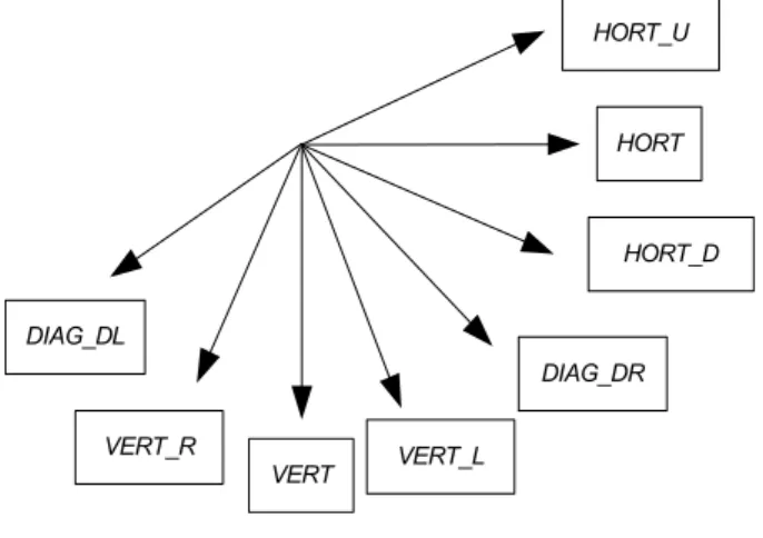
Intra-frame mode has two modes, I4MB and I16MB. I4MB consists of 9 members
which pad elements (a to p) of a 4×4 block with the neighbouring encoded pixels (A to Q) in 8 directions as depicted in Fig. 1-2 and Fig. 1-3, respectively. For instance,
time-consuming, comprising 4 members to predict a 16×16 macroblock as a whole. As for inter-frame mode, it contains the SKIP (direct copy), I4MB, I16MB, and INTER, the most time-consuming mode, which consists of 7 members with different block sizes as shown in Fig. 1-1.
In intra-frame coding, the final mode decision is selected by the member (either from I4MB or I16MB) that minimizes the Lagrangian cost in (1). In inter-frame coding, motion estimations with 7 different block-size patterns, as well as the other members in three members (I4MB, I16MB, and SKIP), are calculated. The final decision is determined by the mode that produces the least Lagrangian cost among the available modes. Currently, the H.264/AVC standard employs a brute force algorithm to search through all the possible candidates and its corresponding members to find an
Fig.1-2 A 4×4 block with elements (a to p) which are predicted by its neighbouring pixels.
a b c d e f g h i j k l m n o p
A B C D E F G H
I J K L
M N O P Q
HORT_U
HORT
HORT_D
DIAG_DR
VERT_L VERT
VERT_R DIAG_DL
Fig. 1-3 Eight direction-biased I4MB members except DC member which is
optimum motion vector [2]. Since the exhaustive search method is employed in all the modes to acquire a final mode decision, the computational burden of the search process is far more significant than any existing video coding algorithm.
1.3 Contributions and organisation of this report
Chapter 2
Proposed intra-frame mode selection
algorithm
2.1 Introduction
In intra-frame coding, the H.264/AVC standard selects a mode which minimizes the Lagrangian cost LCMB as given in (1). The optimisation process entails finding the least distortion while achieving the minimum coding rate. The computation of the distortion parameter, D, requires the availability of the reconstructed image, which means the completion of the encoding-decoding cycle. On the other hand, the evaluation of the rate parameter, R, depends only on the residue blocks obtained from the difference between the original block and the predicted block for each mode by look-up table of the entropy codes. Clearly, the computational requirement of rate evaluation is less demanding than that for the distortion evaluation.
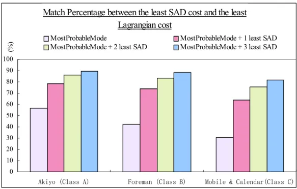
match percentage of 89%, 88% and 81% for the three respective test sequences when the number of candidates increases to 4 including MostProbableMode.
Therefore, to reduce the computational cost of the expensive Lagrangian cost evaluation, we can limit the number of members (say M) that need to undergo the full evaluation process. The M members are those with the least residue energy from amongst all the possible members. Furthermore, the residue blocks of I4MB and I16MB normally have relatively large block energy because there is no prediction. Hence, it is more efficient to operate in the frequency domain rather than in the spatial domain. The following subsections detail the formulation of the fast algorithm.
2.2 Algorithm formulation
The proposed fast intra-mode selection (Fintra) is achieved by selecting fewer members from I4MB mode that need to undergo the full Lagrangian cost evaluation. The selection criterion is the least residue energy which can be measured from the sum of absolute difference (SAD) of the DCT residue block. First, let us denote an
Match Percentage between the least SAD cost and the least Lagrangian cost
0 10 20 30 40 50 60 70 80 90 100
Akiyo (Class A) Foreman (Class B) Mobile & Calendar(Class C)
(%)
MostProbableMode MostProbableMode + 1 least SAD MostProbableMode + 2 least SAD MostProbableMode + 3 least SAD
M×N original block to be BM×N and any intra predicted block to be PM×N,member. For a
unitary transform, the SAD of the DCT residue block is given by
∑
∑
× × = × ×= ( { }, { }) { ( , )}
SADDCT(residue) Diff T BM N T PM N,mode T Diff BM N PM N,member (6)
where Diff(A,B) represents the difference between A and B, where T{.} stands for the unitary transformation. In our case, T{.} stands for the Discrete Cosine Transform (DCT). From (6), a SAD evaluation is equal to the sum of absolute difference
between the transforms of an original DCT-block, T{BM×N} and a predicted
DCT-block, T{PM×N,member}. Then, according to the definition of DCT,
∑
∑
Diff(T{BM×N},T{PM×N,member}) = DCB−DCP,member + ACB −ACP,member (7)Equation (7) indicates that SADDCT(residue) can be obtained by finding the sum of the
absolute differences of both the low-frequency (DC) coefficients and the high-frequency (AC) coefficients. Note that a DC coefficient normally possesses more block energy than the AC coefficients for natural images. Thus, we can formulate the approximation as:
member , member
, member
, )} ' '
, (
{Diff B P DCB DCP ACB ACP
T M×N M×N ≈ − + − , (8)
whereAC 'B represents the AC coefficient that possesses the largest energy of these
AC coefficients in an original DCT-block, and AC'P,member is the AC coefficient that is at the same location as AC 'B in any predicted DCT-block. Since empirical
experiments show that the low-frequency AC coefficients contain more energy than
the high-frequency coefficients, we select AC'B from the lower horizontal and
vertical frequencies, for example, AC(0,1), AC(0,2), AC(0,3) and AC(1,0), AC(2,0), AC(3,0), as the candidates in a 4×4 block. By simple calculations from the 2D-DCT
∑∑
××
= f t
DCB 0 B4 4, , (9)
)] 2 ( ) 1 ( [ )] 3 ( ) 0 ( [ ) 0 , 1
( 1 B B 2 B B
B f r r f r r
AC = × − + × − , (10)
)] 2 ( ) 1 ( [ )] 3 ( ) 0 ( [ ) 1 , 0
( 1 B B 2 B B
B f c c f c c
AC = × − + × − , (11)
)] 3 ( ) 2 ( ) 1 ( ) 0 ( [ ) 0 , 2
( 0 B B B B
B f r r r r
AC = × − − + , (12)
)] 3 ( ) 2 ( ) 1 ( ) 0 ( [ ) 2 , 0
( 0 B B B B
B f c c c c
AC = × − − + , (13)
)] 2 ( ) 1 ( [ )] 3 ( ) 0 ( [ ) 0 , 3
( 2 B B 1 B B
B f r r f r r
AC = × − + × − , (14)
)] 2 ( ) 1 ( [ )] 3 ( ) 0 ( [ ) 3 , 0
( 2 B B 1 B B
B f c c f c c
AC = × − + × − , (15)
where f0, f1, f2are scalars and the values are 0.2500, 0.3267 and 0.1353, respectively.
) (m
rB and cB(n) represent the sum of the image intensities in the mth row and nth
column of B4×4, respectively (refer to Fig. 2). For example, rB(0)=a+b+c+d. Next, we consider how to efficiently access the DCP,member and AC'P,member values of the predicted block, P4×4,member. Unlike the original block, the predicted blocks are
the direction-biased paddings from the neighbouring pixels. In order to simplify the calculation, we rewrite each of the equations of (9) to (15) in matrix form, i.e.,
Θ = • p a AC AC M M ) ' ( POS member ,
'P B , (16)
where POS(AC'B) stands for position of AC'B and ΘPOS(AC'B) =
[
θ1,θ2,K,θ16]
is atime-frequency conversion transpose vector between an AC'P and the predicted elements (a to p). For instance, if POS(AC'B) is selected at (2,0), then according to
(12) ] ,.., , ., ,... , ,.., [ 4 0 0 8 0 0 4 0 0 ) 0 , 2
( = 1f 23f 1− f4 24 4 34−f 1f 23f
In a similar manner, a matrix formula can be provided to relate the predicted elements and the neighbouring samples (A to Q):
= = • Q A C C C C C C C C C C C C Q A p a M M M L O M O M O L M M M M M 17 , 16 16 , 16 2 , 16 1 , 16 17 , 15 1 , 15 17 , 2 1 , 2 17 , 1 16 , 1 2 , 1 1 , 1 member
C , (18)
where Cmember is a 16-by-17 conversion matrix, for instance, CHORT, the conversion
matrix of the horizontal member, pads the horizontal pixel I to the first row’s
elements, i.e., a to d. Then, all the coefficients in the first 4 rows of CHORT are zero
except for the ninth coefficients (C1,9, C2,9, C3,9, C4,9, i.e., position of I ), which are
one.
We then obtain the relationship between AC'P,member and the neighbouring pixels
(A to Q) by combining (16) and (18).
= • Q A AC AC M M ) ' POS( , member
'P ω B , (19)
where member ,POS( ' )
Β
ω AC is a 1-by-17 transpose vector. By arranging the elements of
) ' POS( , member Β
ω AC to form a matrix, we can obtain the values of AC'P,member for all the nine I4MB members.
• = Q A AC AC AC AC M M M POS( ' )
9 member , 2 member , 1 member , ' ' ' B Ω P P P
, (20)
= ) ' POS( , 9 member ) ' POS( , 2 member ) ' POS( 1, member ) ' ( POS B B B B ω ω ω Ω AC AC AC AC
M . (21)
) ' ( POS B
Ω AC in (21) is a 9-by-17 sparse matrix. Similarly, ΩDC exists to obtain the
values of DCP,member for the 9 prediction modes.
• = Q A DC DC DC DC M M M Ω P P P 9 member , 2 member , 1 member , ' ' '
, (22)
and ΩDC can be deduced in a similar manner from (9), (16), and (18).
= C , 9 member C , 2 member C 1, member D D D DC ω ω ω Ω
M , (23)
where, × × × × × × × × × × × × = 17 , 16 0 16 , 16 0 2 , 16 0 1 , 16 0 17 , 15 0 1 , 15 0 0 17 , 2 0 1 , 2 0 17 , 1 0 16 , 1 0 2 , 1 0 1 , 1 0 member, C f C f C f C f C f C f C f C f C f C f C f C f DC L O M O M O L
ω . (24)
Note that ΩDC and all six POS( ' )
B
Ω AC can be calculated and stored in advance.
2.3 Proposed fast Algorithm
MostProbableMode (the mode predicted from use of prior knowledge of neighbouring blocks) has a higher chance of being selected as the prediction mode, it is included in the short-listed candidates although it may not produce the least residue energy. The proposed algorithm is summarized as follows:
A1. Evaluate (9)-(15) to obtain DCB and an AC'B, the AC coefficient which
possesses the largest AC energy of the original block.
A2. Calculate values of DCP,member and AC'P,member of the 9 predicted blocks by utilizing (22) and (20).
A3. Apply SAD evaluation in (8) to shortlist 1-4 candidates with the smallest residue energies (including MostProbableMode).
A4. Select a prediction mode that minimizes (1) from the short-listed candidates.
The proposed intra-frame mode selection algorithm, Fintra, employs the inherent frequency characteristic of an original block and its predicted block without any a priori knowledge, such as predefined threshold or other priori macroblock information. This feature is considered one of the main advantages of the proposed algorithm in that it can be easily applied to the I16MB and mode selection for chrominance components from one sequence to another. Furthermore, the matrices, all POS( ' )
B Ω AC in
different AC'B positions andΩDC, can be calculated and stored in advance.
2.4 Simulation results
All the simulations presented in this section were programmed using C++. The computer used for the simulations was a 2.8GHz Pentium 4 with 1024MB RAM. The testing benchmark was the JM6.1e version provided by the Joint Video Team (JVT) [12]. The selected sequences in 2 different resolutions, namely, QCIF (144×176) and
all sequences were quantized by a static Qp factor of 32. They were encoded by the intra-coding technique provided by JM6.1e and the proposed Fintra algorithm. In each case, the rate was 30 frames per second with no skip frame throughout the 30 frames.
TABLE 2-1
Simulation results of the proposed Fintra algorithm compared with JM6.1e, the H.264/AVC software, in three sequence classes and two resolutions.
Classes / Sequences Resolutions (pels)
Y-PSNR Difference
(dB)
Bit Rate Difference
(%)
Speed-up cf.JM6.1e
(%) Akiyo 144×176 -0.01 dB 0.24% 51.85% Grandma 144×176 -0.02 dB 0.50% 51.59% Hall Monitor 288×352 -0.02 dB 0.33% 59.40% A
Mother & Daughter 288×352 -0.01 dB 0.31% 57.98%
City 288×352 -0.04 dB 0.19% 54.65% Coastguard 144×176 -0.03 dB -0.18% 54.95%
Foreman 288×352 -0.02 dB 0.26% 59.13% News 144×176 -0.04 dB 0.28% 53.90%
B
Paris 288×352 -0.04 dB 0.21% 59.97% Car Phone 144×176 -0.01 dB 0.49% 51.75%
Crew 288×352 -0.01 dB 0.21% 55.10% Harbour 288×352 -0.03 dB 0.14% 61.50%
Football 144×176 -0.05 dB 0.43% 52.42% Mobile & Calendar 288×352 -0.09 dB 0.16% 55.17%
Table Tennis 288×352 -0.01 dB 0.01% 51.92% C
Waterfall 288×352 -0.04 dB 0.03% 55.05%
Table 2-1 shows the simulation results of the proposed Fintra algorithm in comparison with the JM6.1e implementation. Comparisons are given for PSNR difference in the luminance component, Y-PSNR (measured in dB), bit rate difference (as a percentage), and speedup (computational performance). The Table 2 entries are arranged according to class of sequence.
Chapter 3
Proposed inter-frame mode selection
algorithms
3.1 Introduction
Success of two proposed fast mode selection algorithms, Finter1 and Finter2, for inter-frame coding is achieved by discarding the least possible block size. Mode knowledge of the previously encoded frame(s) is employed by the proposed Finter1 algorithm, whereas the Finter2 algorithm incorporates temporal similarity detection and the detection of different moving features within a macroblock. However, both Finter1 and Finter2 make use of a general tendency: a mode having a smaller partition size may be beneficial for detailed areas during the motion estimation process, whereas a larger partition size is more suitable for homogeneous areas [7]. Therefore the primary goal is to determine a complexity measurement for each macroblock.
3.2 Algorithm formulation
In this subsection, we derive a low-cost complexity measurement based on summing the total energy of the AC coefficients to estimate the block detail. The AC coefficients are obtained from the DCT coefficients of each block. The definition is
( )
∑
−−
≠ ∪
= 1, 1
0 2
N M
v u
uv
AC F
E , (25)
∑ ∑
− = − = + + = 1 0 1 0 16 ) 1 2 ( cos 16 ) 1 2 ( cos ) ( ) ( N n M m mn uv v n u m I v c u cF π π , (26)
and, 0 , 0 , 2 , 2 1 , 1 ) ( ), ( ≠ = = v u for v u for N M N M v c u
c , (27)
and Imn stands for the luminance intensity located at (m,n) of an M×N block.
From (25), the total energy of the AC components, EAC, of an M×N block is the sum of all the DCT coefficients, Fuv, except for the DC component, u = 0 and v = 0.
According to the energy conservation principle, the total energy of an M×N block is equal to the accumulated energy of its DCT coefficients. Thus, (25) can be further simplified as
( )
1 20 1 0 1 0 1 0
2 1 1
− =
∑∑
∑ ∑
− = − = − = − = N n M m mn M m N n mnAC I M N I
E , (28)
where the first term is the total energy of the luminance intensities within an M×N block, and the second term represents the mean square intensity. (28) clearly shows that the energy of the AC components of a macroblock can be represented by the variance.
= − = − − =
∑
∑
∑
∑
= − + = − + = = c) -(29 } 16 , , 1 { , 4 1 b) -(29 } 4 , , 1 { , 8 1 a) -(29 16 1 2 4 1 2 16 1 ) 1 ( 4 ) 1 ( 4 16 1 2 16 1 L L x S E n S E S E E x x x x x n x n x x x x ACwhere En={e1, e2, …, e16} and Sn={s1, s2, …, s16} represent the sum of energies and
intensities of the 4×4 blocks decomposed from a macroblock respectively, with the scanning pattern shown in Fig. 3-1. The first piecewise equation is applied to a macroblock with block size of 16×16 pixels; the second is for 4 blocks, n = {1, 2, 3, 4}
of 8×8 pixels; and the last is applicable to the 16 decomposed 4×4 blocks.
Evaluating the maximum sum of the AC components is the next target. By definition, the largest variance is obtained from the block comprising a checkerboard pattern in which every adjacent pixel is the permissible maximum (Imax) and minimum
(Imin) value alternately [8]. Thus, Emax, the maximum sum of AC components of an
M×N block is
(
) (
)
2 2 1 2 min max 2 min 2 max max N M I I I IE = + − + × × . (30)
Note that Emax can be calculated in advance. Then the criterion to assess the
complexity RB of a macroblock MB is
) ln( ) ln( max E E R AC
B = . (31)
The function of the natural logarithm is to linearise both Emax and EAC such that the
3.3 The proposed Finter1 algorithm
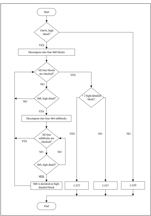
Fig. 3-2 shows the flowchart of the proposed Finter1 algorithm that incorporates the complexity measurement. In total, 7 partition sizes are recommended by H.264/AVC for P-frames, namely, 16×16, 16×8, 8×16, 8×8, 8×4, 4×8, 4×4 as well as SKIP, 4MB and 16MB. However, in our complexity measurement, only 3
categories, of sizes of 16×16, 8×8, and 4×4, respectively, are selected as test block sizes. We denote them as Cat0, Cat1, and Cat2, respectively.
The proposed Finter1 algorithm provides a recursive way to determine the
complexity of each macroblock. Firstly, a macroblock of 16×16 pixels is examined with (29-a). A Cat0 tag is given if it is recognized as being a homogenous macroblock. Otherwise, the macroblock is decomposed into 4 blocks of 8×8 pixels. Note that an
8×8 block is recognized as high-detailed if it satisfies two conditions: (a) theRB in (31)
is greater than 0.75, and it is decomposed into four 4×4 blocks, and (b) one of its four
decomposed 4×4 blocks is high-detailed as well. If an 8×8 block satisfies the first condition but not the second, it is still recognized as low-detailed. After checking all the 8×8 blocks, a Cat2 tag is given to a macroblock which possesses more than two high-detailed blocks, otherwise a Cat1 tag is assigned. Table 3-1 displays the relationship between the three categories in the proposed algorithm and the nine members of the inter-frame modes. It is observed that the Cat0 category covers the
1 2
3 4
5 6
7 8
9 10 11 12
13 14 15 16
least number of members of the inter-frame mode, whereas the Cat2 category contains all the available members. The table further indicates that the higher detailed the macroblocks are, the more prediction modes the proposed algorithm has to check.
TABLE 3-1
The relationship between the three categories in the proposed algorithm and the 9 members of inter-framemodes.
Mode knowledge of previously encoded frame(s):
A trade-off between efficiency and prediction accuracy exists. If a Cat2 category is assigned less often, the efficiency of the algorithm will increase, but the chance of erroneous prediction also increases. An improved method is proposed, that considers the mode knowledge at the same location in the previously encoded frame. Since most of the macroblocks are correlated temporally, it is easy to see that the mode decision in the previous frame contributes reliable information for revising the erroneous prediction that may be indicated by its intrinsic complexity information. Therefore, our suggestion is first to convert all the mode decisions in the previous frame into the corresponding categories. Then, the prediction is revised to the higher category if that of the corresponding historic data is higher than the current predictor. However, no action is taken if the reverse situation is true.
The algorithm of Finter1:
Cat0 category algorithm:
B1. Obtain a motion vector for a 16×16 macroblock by using the full search algorithm with search range of ±8 pixels.
B2. The best prediction of I4MB and I16MB can be obtained by applying steps A1 to A4 and the full search algorithm, respectively.
Category Corresponding Modes
Cat0 16×16, SKIP, I16MB, I4MB
Cat1 16×16, 16×8, 8×16, 8×8, SKIP, I16MB, I4MB
B3. Compute the Lagrangian costs of SKIP, I4MB, I16MB, and INTER to find a
Start
16x16, high detail?
Decompose into four 8x8 blocks
8x8, high detail?
Decompose into four 4x4 subblocks
4x4, high detail? All four blocks
are checked?
All four subblocks are
checked?
8x8 is declared as high-detailed block
> 2 high-detailed block?
CAT2 CAT1 CAT0
End
NO NO
YES NO
NO NO
NO
YES
YES
YES
YES
YES
final mode decision for the current macroblock.
Cat1 category algorithm:
C1. Obtain a motion vector for each of the four 8×8 blocks in a macroblock by using the full search algorithm with search range of ±8 pixels.
C2. Continue to search for motion vector(s) for the 8×16 blocks, 16×8 blocks, and
16×16 macroblocks by referring only to the 4 search points, i.e., the motion
vectors of the four 8×8 blocks.
C3. Perform step B2 to B3 to find the final mode decision for the current macroblock.
Cat2 category algorithm:
D1. Obtain a motion vector for each of the sixteen 4×4 blocks in a macroblock by using the full search algorithm with search range of ±8 pixels.
D2. Continue to search for motion vector(s) for 8×4 blocks, 4×8 blocks, and 8×8 blocks by referring only to the 16 search points, i.e., the motion vectors of the sixteen 4×4 blocks.
D3. Perform the steps C2 to C3 to find the final mode decision for the current macroblock.
3.4 The proposed Finter2 algorithm
The efficiency of the proposed Finter2 is achieved by introducing two additional measurements targeted at two kinds of encoded macroblocks: (a) macroblocks encoded with SKIP mode (direct copy from the corresponding macroblock located at the same position in the previous frame); (b) macroblocks encoded by the inter-frame modes with larger decomposed partition size (greater than 8×8 pixels). By successfully identifying these two kinds of macroblocks, the encoder is exempted from examining them with all possible inter-frame modes, which saves encoding time.
Measurement of temporal similarity:
The SKIP mode is normally assigned to a macroblock that comprises almost
position in the previous frame, for example in areas representing a static background.
The macroblocks coded with SKIP mode (skipped macroblocks) can be easily
detected by comparing the residue between the current macroblock and the previously encoded macroblock with a threshold as follows:
> < =
Th S
Th S
S T
residue residue residue 0,
, 1 )
( (32)
∑∑
− −= m n
1 t n m t n m
Sresidue B , , B , , (33)
where Sresidue is the sum absolute difference between Bm,n,t and Bm,n,t-1, which represent current and previous macroblocks, respectively. If T(Sresidue) = 1, the current
macroblock is a skipped macroblock. However, performing this calculation for every macroblock further increases the encoding time. Lim et al. [10] suggested performing temporal similarity checking if the current 16×16 macroblock has zero motion. This necessitates each macroblock, including skipped macroblocks, to undergo at least one complete cycle of motion estimation. If the encoder can detect the skipped macroblocks without a priori knowledge, then a significant proportion of the encoding time will be saved.
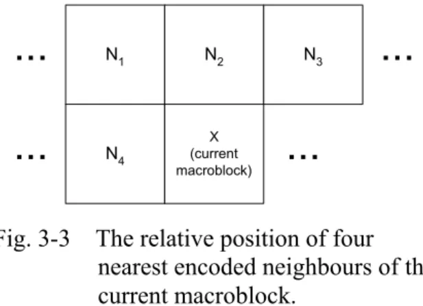
Generally, the skipped macroblocks tend to occur in clusters, such as in a patch of static background. Thus, we propose that the current macroblock has to undergo temporal similarity detection if one of the encoded neighbours is a skipped macroblock. The temporal similarity detection is implemented according to (32) and (33), but we propose an adaptive spatially varying threshold, ThASV, to replace Th.
(
1 2 3 4)
ASV C*min SN ,SN ,SN ,SN
Th = (34)
where C is a constant; SN1, SN2, SN3, and SN4 are the sum absolute difference of four
nearest encoded neighbours, N1, N2, N3, N4, as shown in Fig. 3-3. They are valid and
Measurement on block-based motion consistency:
The tendency that the inter-frame modes with larger partition size (of sizes 8×8, 8×16, 16×8, and 16×16 pixels) are more suitable to encode homogeneous macroblocks has been verified by a number of authors [7,10-11]. By contrast, macroblocks containing moving features appear more detailed and therefore require use of smaller block sizes. Thus, the proposed algorithm suggests checking the motion vector of each 8×8 block decomposed from a highly detailed macroblock. If consistency among motion vectors exists, the proposed algorithm checks the inter-modes with partition size greater than 8×8, otherwise, all possible inter-frame inter-modes are searched.
The algorithm of Finter2:
Fig. 3-4 shows a flowchart of the proposed Finter2 algorithm, which is
summarized as follows:
E.1. Turn off all flags including SKIP, INTRA and all inter-modes
E.2. Check if one of the four nearest neighbours of the current macroblock is a skipped macroblock. Implement E.3 if the situation is true. If not, go to E4. E.3. Obtain a threshold, ThASV, from (34). Compare ThASV with the sum absolute
difference between the current macroblock and the previous macroblock at the same position. If the sum is smaller than the threshold, turn on the flag for SKIP only. Otherwise, continue to E.4.
N1 N2 N3
N4 (currentX macroblock)
...
...
...
...
E.4. Check the complexity of the macroblock using equation (29-a) and (31). If the current macroblock is homogeneous, turn on the flag for I4MB, I16MB and the inter-mode with partition size 16×16. Otherwise, continue to E.5. E.5. Decompose the highly detailed macroblock into four non-overlapping 8×8
blocks. Check whether the motion vectors of the four blocks are consistent. If
Fig. 3-4 Flowchart of the proposed Finter2 algorithm incorporating the complexity measurement for a macroblock, temporal similarity, and the detection of different moving features within a macroblock.
Start
Is any neighbour SKIPPED ?
MBcurr-MBprev< ThASV
Set SKIPPED and INTRA modes on
Turn all flags off
Check the complexity of
current MB
homogeneous ?
Set 16x16, SKIPPED and INTRA modes on
Set 8x8 mode on and apply ME
Are all MVs consistent?
Set 16x16, 16x8, 8x16, SKIPPED, and INTRA
modes on
Set all modes on YES
YES
YES NO
NO NO
End YES
consistent, check the flags of I4MB, I16MB, and the inter-modes with partition size 8×16, 16×8, and 16×16 and go to E.7. Otherwise, continue to E.6.
E.6. Turn on all flags and use sixteen motion vectors obtained from inter-modes with partition size 4×4 as searching points for the inter-mode with partition size 4×8 and 8×4 rather than performing full search. Then, continue to E.7. E.7. Utilise the four motion vectors obtained from four 8×8 blocks as searching
points for the inter-modes with partition size 8×16, 16×8, and 16×16 rather than performing full search.
3.5 Simulation results
This section compares two simulation results employing the proposed Finter1 and Finter2 algorithms. The settings of the simulations are as follows: all the sequences are defined in a static coding structure, i.e., one I-frame is followed by nine P-frames (1I9P), with a frame rate of 30 frames per second and no skip frame throughout the 100 frames. The precision and search range of the motion estimation is set to ¼ pixel and ±8 pixels, respectively. Lastly, Context-based Adaptive Binary Arithmetic Coding (CABAC) is used to perform entropy coding and a static quantizer value, Qp = 29, is applied throughout the simulation.
The table summarises the simulation results of the two algorithms – Finter1 and Finter2 in terms of PSNR difference, bit rate difference and speed up compared with JM6.1e, the testing benchmark. The general trends are identified as follows: both fast algorithms introduce less than 0.08 dB of PSNR degradation in Class A and Class B, and approximately 0.10 dB in Class C. Note that there is insignificant PSNR difference between the MFInterms and FInterms algorithms. As to compression ratio, the proposed MFInterms produces slightly higher bit rates than FInterms especially in the Class C sequences, however the bit differences for most test sequences are less than 5%. Nevertheless, the picture degradations and bit rate increase are generally considered within acceptable range as human visual perception is unable to distinguish a PSNR difference of less than 0.2dB.
algorithm provided improvements of only 18-25% and 22-31%, respectively. The reason that a significant proportion of the encoding time is saved with the MFInterms algorithm is that skipped macroblocks are detected accurately and are encoded with
SKIP mode, obviating the need for other mode examinations. As a result, the
encoding time of a P frame could be shorter than that of an I frame if a sequence contains a significant number of skipped macroblocks.
TABLE 3-2
Simulation results of the proposed Finter1 and Finter2 algorithms compared with JM6.1e, the H.264/AVC software, in three sequence classes.
PSNR Difference Bit Rate Difference Speed up cf. JM6.1e Sequences
Finter1 Finter2 Finter1 Finter2 Finter1 Finter2
Ship Container -0.02 dB -0.06 dB 0.10 % 0.37% 30.85% 72.94%
A
Sean -0.05 dB -0.07 dB 0.44 % -0.11% 29.87% 69.63%
Silent -0.07 dB -0.08 dB 1.47 % 3.73% 26.64% 60.22%
B
News -0.07 dB -0.07 dB 1.34 % 1.52% 22.04% 62.08%
Stefan -0.09 dB -0.13 dB 5.36 % 8.90% 18.34% 28.72%
C
Chapter 4
Comparison results of the combined
algorithms
This section presents two sets of simulation results employing the proposed combinations of (Fintra + Finter1) algorithms and (Fintra + Finter2) algorithms for inter-frame coding, as P-frames may contain I-macroblocks. All the simulations were programmed using C++. The computer used for the simulations was a 2.8GHz Pentium 4 with 1024MB RAM. The testing benchmark was the JM6.1e version provided by the Joint Video Team (JVT) [12]. The selected sequences in 2 different
resolutions, namely, QCIF (144×176) and CIF (288×352) formats, are classified into three different classes, i.e., Class A, which are sequences containing only low spatial correlation and motion, e.g., Akiyo and Ship Container; Class B, which contains medium spatial correction and/or motion, e.g., Foreman and Silent Voice; and Class C, where high spatial correlation and/or motion are involved, e.g., Mobile & Calendar and Stefan. In the following simulations, 22 test sequences in different resolutions are presented. Fig. 4-1 shows snapshot frames from the less common sequences used.
presented in terms of an average PSNR of the luminance and two chrominance components, i.e., Y, U, and V (measured in dB) rather than the PSNR of the luminance component (Y-PSNR).
Table 4-1 summarise the performance of two proposed combinations of algorithms, (Fintra + Finter1) and (Fintra + Finter2). The general trends are identified as follows: on average, there is a degradation of 0.02 dB in Class A, and approximately 0.05dB - 0.06 dB in other classes for both proposed combinations of algorithms. It is clear that the average PSNR difference between two proposed combinations of algorithms is insignificant (less than 0.02 dB). As to compression ratio, the tendency of a slight bit increase is directly proportional to the class of sequence. The test sequences of Class A attain the least bit increase, whereas the high motion sequences in Class B and Class C produce slightly higher bit rates than the H.264/AVC standard. However, the bit differences for most test sequences are still within an acceptable range of less than 5%. In general, the combination of (Fintra + Finter2) performs better in terms of compression than the combination of (Fintra + Finter1). The degradations and the bit differences are due to the erroneous prediction in the proposed combined algorithms. Nevertheless, the degradations are still below
the human visual threshold, which is widely recognised as being less than 0.15-0.20 dB.
TABLE 4-1
Simulation results of the two proposed combined algorithms, namely, Fintra + Finter1 and Fintra + Finter2, versus the JM6.1e, H.264/AVC software, for three
sequence classes and two resolutions.
Average PSNR Difference (dB)
Bit Rate Difference (%)
Speed-up cf. JM6.1e (%) Classes / Sequences Resolution (pels)
Fintra +
Finter1 Fintra Finter2 + Fintra + Finter1 Fintra Finter2 + Fintra + Finter1 Fintra Finter2 +
Akiyo 288×352 -0.01 dB -0.02 dB 2.02% 0.75% 61.83% 81.64% Container Ship 144×176 -0.03 dB -0.03 dB 1.60% 0.81% 60.35% 82.55% Grandma 144×176 -0.02 dB -0.02 dB 1.26% -0.02% 62.94% 79.86% A
Sean 144×176 -0.03 dB -0.04 dB 2.11% 0.38% 60.19% 86.61% City 288×352 -0.04 dB -0.05 dB 4.70% 4.10% 57.06% 63.00% Coastguard 144×176 -0.03 dB -0.05 dB 6.47% 7.26% 55.53% 59.53% Foreman 288×352 -0.06 dB -0.08 dB 7.21% 6.53% 62.00% 66.00% News 144×176 -0.06 dB -0.07 dB 3.17% 2.05% 60.36% 79.27% Paris 288×352 -0.03 dB -0.05 dB 3.76% 3.74% 49.78% 71.66% B
Silent Voice 144×176 -0.04 dB -0.05 dB 3.86% 4.75% 44.93% 67.35% Car Phone 144×176 -0.09 dB -0.10 dB 4.50% 3.50% 58.87% 62.17% Football 144×176 -0.09 dB -0.11 dB 5.36% 6.78% 53.29% 50.54% Harbour 288×352 -0.05 dB -0.04 dB 2.62% 0.59% 51.16% 52.39% Mobile & Calendar 144×176 -0.05 dB -0.05 dB 2.33% 0.25% 51.53% 53.97% Stefan 288×352 -0.05 dB -0.07 dB 2.01% 2.07% 52.17% 54.61% Table Tennis 144×176 -0.06 dB -0.06 dB 6.87% 6.63% 58.98% 70.06% Template 288×352 -0.07 dB -0.08 dB 2.29% 0.53% 54.65% 54.32% C
Waterfall 288×352 -0.02 dB -0.02 dB 2.06% 0.79% 57.69% 68.00%
Chapter 5
Conclusions and future prospects
5.1 Main contributions
In this report, we proposed three fast algorithms, namely, Fintra, Finter1, and Finter2, for fast mode selection in the H.264/AVC standard. The algorithms improve the computational performance of both intra- and inter-frame coding, thus reducing the implementation requirements in real applications. Improvement is accomplished by discarding the least possible modes to be selected. The Fintra algorithm intelligently selects fewer candidate members need to undergo expensive Lagrangian evaluation. The Finter algorithms utilise a complexity measure to identify those low detailed macroblocks that require less demanding processing. The results of extensive simulations demonstrate that the proposed algorithms can attain a time saving of up to 62% and 86% in intra-coding and inter-coding, respectively, compared with JM6.1e, the benchmark. This is achieved without sacrificing both picture quality and bit rate efficiency.
5.2 Timetable of the previous research projects
I joined the department of Computer Science at the University of Warwick on 1st October 2003. It has been nine months until the end of June 2004.
TABLE 5-1
The table specifies the important events and the dates October 2003 to June 2004. Date/Period Descriptions 01st Oct. 2003 Joined Department of Computer Science at Warwick University
24th Oct. 2003 Submitted a paper to Speech and Signal ProcessingIEEE International Conference on Acoustics, (ICASSP) 2004 in Montreal, Canada.
04th Nov. 2003 Conducted a group seminar for multimedia group in Department of Computer Science.
15th Dec. 2003 Submitted a paper to Multimedia and Expo IEEE International Conference on (ICME) 2004 in Taipei, Taiwan. 09th Jan. 2004 A paper was accepted by ICASSP 2004.
01st Mar. 2004 A paper was accepted by ICME 2004. Dec. 2003 –
Mar 2004 Worked on progressive fast algorithm for inter-frames in H.264/AVC.
15th Mar. 2004 Submitted two papers to Processing (ICIP) 2004 in Singapore. IEEE International Conference on Image
01st May 2004
Submitted one paper to Special Issue on Emerging H.264/AVC video coding of Journal of Visual Communication and Image Representation.
20th May 2004 A paper was accepted by ICIP 2004. Another was rejected. 30th Jun. 2004 A presentation was given on Postgraduate Research Day.
May 2004 –
June 2004 A new project, scalable video coding, is started.
5.3 Future prospects
My future research interests will focus on the emerging video coding standard, Scalable Video Coding (SVC), the most recent standard, which is championed by the Joint Video Team (JVT), a collaboration team of two international standard bodies, ITU-T VCEG and ISO/IEC MPEG.
The procedure of ASVC standard
Institute (HHI) of Germany, Microsoft Research Asia (MSRA), National Chiao-Tung University (NCTU) of Taiwan, and Poznań University of Technology (PU) of Poland [16]. In late March, the JVT called for another proposal on core experiments (CE) of ASVC standard. The CEs aim at obtaining significant improvements in four parts of the ASVC standard: scalable motion information (CE1a), spatial transform and entropy coding (CE1b), intra modes (CE1c), base-layer of scalable video (CE1d). The details of each CE are elaborated in Table 5-2.
Since core experiments CE1a and CE1c have some correlation with my previous research interest, my research will concentrate on these two core experiments. The two major research works include: (1) studying and learning how to utilise the codec of the CE provided by MPEG SVC group, (2) improving the performance of the state-of-the-art scalable video techniques.
TABLE 5-2
The table describes the Core Experiments of MPEG SVC proposed by JVT.
Core Experiments (CE) Descriptions
a. Scalable motion information
Evaluating the optimum trade-off between motion data and texture data depending on the spatial-temporal-SNR resolution.
b. Spatial transform and entropy coding
Evaluating different spatial transforms and associated entropy coding techniques.
c. Intra modes Improving coding efficiency using intra coding.
d. Introduction of a base-layer
Improving the performance of the scalable coder at low resolutions (low image size and frame rate). 1
e. MCTF with deblocking
Improving visual quality and coding efficiency by reducing artefacts occurring in t+2D wavelet video coding schemes with block-based motion
compensation.
2 AVC-based CE NIL
3 Quality evaluation Ensuring that the above visual quality evaluation method for the CE is valid.
The structure of the scalable video coding