warwick.ac.uk/lib-publications
A Thesis Submitted for the Degree of PhD at the University of Warwick
Permanent WRAP URL:
http://wrap.warwick.ac.uk/109582
Copyright and reuse:
This thesis is made available online and is protected by original copyright. Please scroll down to view the document itself.
Please refer to the repository record for this item for information to help you to cite it. Our policy information is available from the repository home page.
THE BRITISH LIBRARY
BRITISH THESIS SERVICE
TITLE THE EFFECTS OF ROTATION AND WALL
COMPLIANCE ON HYDRODYNAMIC STABILITY
A U TH O R Alison J.
COOPER
DEGREE Ph.D
A W A R DING Warwick University BODY
DATE 1996
TH ESIS DX207686
NUM BER
THIS THESIS HAS BEEN MICROFILMED EXACTLY AS RECEIVED
The quality of this reproduction is dependent upon the quality of the original thesis submitted for microfilming. Every effort has been made to ensure the highest quality of reproduction. Some pages may have indistinct print, especially if the original papers were poorly produced or if the awarding body sent an inferior copy. If pages are missing, please contact the awarding body which submitted the degree.
Previously copyrighted materials (Journal articles, published texts, etc.) are not filmed.
This copy of the thesis has been supplied on condition that anyone who consults it is understood to recognise that its copyright rests with the author and that no information derived from it may be published without the author's prior written consent
THE EFFECTS OF ROTATION AND
WALL COM PLIANCE ON
HYDRODYNAM IC STABILITY
A L IS O N J. C O O P E R
B.Sc. (Hons)
A thesis subm itted for the degree of Doctor of Philosophy
Department of Engineering
University of Warwick
Coventry CV4 7AL
CONTENTS
List of Figures. v
List of Tables. viii
Acknowlegements. ix
Declaration. x
Summary. xi
1. Introduction. 1
1.1. General Overview. 1
1.2. Motivation. 2
1.2.1. The Effects of Rotation on Plane Channel Flow. 3
1.2.2. The Effects of Wall Compliance on Boundary Layer Stability. 4
1.3. Outline of Contents. 8
2. Stability of Rotating Channel Flow. 10
2.1. Introduction. 10
2.2. Review of Theoretical and Experimental Works. 11
2.3. Channel Geometry and Governing Equations. 18
2.4. Linear Stability Analysis. 20
2.5. Numerical Method - Spectral Techniques. 21
2.5.1. Chebyshev Collocation. 22
2.6. Application of Spectral Collocation to Rotating Channel Problem. 25
2.7. Code Validation. 28
2.8. Stability Results for Family of Velocity Profiles. 28
2.9. Algorithm to Determine Minimum Point of Neutral Surface. 32
2.10. Weakly Nonlinear Theory. 37
2.11. Derivation of the Ginzburg-Landau Equation. 38
2.12. Numerical Solution to Singular Systems. 45
2.13. Terms Vanishing in the Solvability Condition. 46
2.14. Summary. 48
3. The Effect of Wall Compliance on the Rayleigh Instability.
Part 1 : Inviscid Analysis. 49
3.1. Introduction. 49
3.2. Classification of Instabilities. 50
3.2.1. Convective and Absolute Instability. 50
3.2.2. Wall-based and Flow-based Instability. 50
3.2.3. Energy Classification. 51
3.3. Boundary Layer in an Adverse Pressure Gradient. 52
3.4. Instability of Two-Dimensional Parallel Flows at Infinite Reynolds Number. 53
3.5. Formulation of Global Eigenvalue Scheme. 56
3.6. Results for Rigid Wall. 59
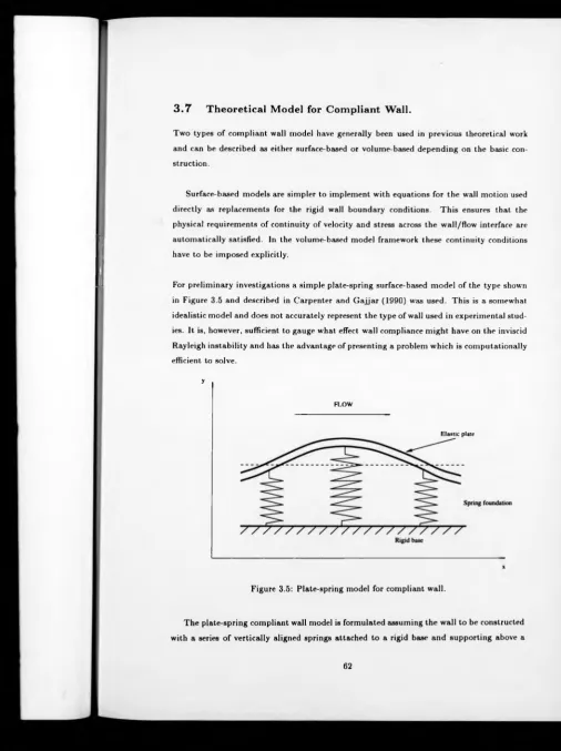
3.7. Theoretical Model for Compliant Wall. 62
3.8. Optimal Wall Properties. 66
3.9. Hydroelastic Instabilities. 72
3.9.1. Results. 72
3.10. Summary. 77
4. The Effect of Wall Compliance on the Rayleigh Instability.
Part 2 : Viscous Analysis. 79
4.1. Introduction. 79
4.2. Falkner-Skan Velocity Profiles. 80
4.3. Flow Disturbance Equations. 82
4.4. Formulation of the Rigid Wall Eigenvalue Problem. 83
4.4.1. Integration of the Orr-Sommerfeld Equation. 83
4.4.2. Numerical Method - Gram-Schmidt Orthonormalisation. 85
4.5. Comparison With Existing Results for the Rigid Wall. 87
4.6. Volume-based Compliant Wall. 87
4.7. Governing Equations for the Wall Motion. 89
4.8. Coupling of Wall and Flow Equations. 92
4.9. Boundary Conditions for the Orr-Sommerfeld Equation. 93
4.10. Wall Parameters. 95
4.11. Code Validation. 95
4.12. Growth Rates Obtained Using Optimal Wall Properties. 97
4.13. Determining the Eigenfunctions. 102
4.13.2. Wall Eigenfunctions. 105
4.14. Energy Balance Equation. 108
4.15. Summary. 113
5. Instabilities in the Rotating Disc Boundary layer. 114
5.1. Three-dimensional Instability. 114
5.2. Review of Work on the Rotating Disc. 116
6. The Effects of Wall Compliance on Instability in Rotating Disc Flow. 131
6.1. Introduction. 131
6.2. Mean Flow Field. 133
6.3. Governing Stability Equations. 134
6.4. Numerical Solution of the Stability Equations. 137
6.5. Wall Equations. 142
6.6. Coupling Fluid and Wall Equations. 146
6.6.1. Numerical Aspects of the Coupled Problem. 148
6.6.2. Calculation of Eigenfunctions. 149
6.7. Validation of Rotating Disc/Compliant Wall Code. 149
6.8. Results for Stationary Modes. 150
6.8.1. General Results. 150
6.8.2. Stability Results for the Type 1 Instability. 152
6.8.3. Stability Results for the Type 2 Instability. 160
6.9. Energy Equation. 162
6.9.1. Energy Results for Stationary Modes. 166
6.10. Stationary Vortex Structures. 172
6.11. Stability Results for Travelling-wave Modes. 173
6.11.1. Stability Results Using the Orr-Sommerfeld Equation. 177
6.11.2. Type 1/Type 2 Response to Wall Compliance. 179
6.11.3. Energy Results for Travelling-wave Modes. 187
6.12. Wall-based Instability. 192
6.13. Summary. 196
7.1. Stability Features of Rotating Channel Flow. 199
7.2. Wall Compliance Effects on the Rayleigh Instability. 200
7.3. Effect of Wall Compliance on Instability in Three-Dimensional
Boundary Layers. 202
References 207
Appendix A. 216
Appendix B. 218
LIST OF FIGURES
2.1. Geometry and coordinate system for rotating channel. 18
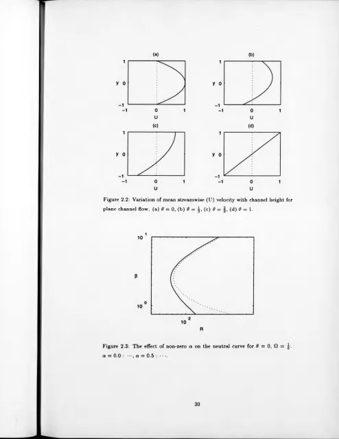
2.2. Streamwise velocity profiles for plane channel flow. 30
2.3. The effect of non-zero a on the neutral curve. 30
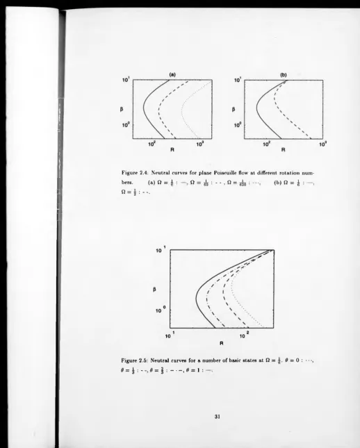
2.4. Neutral curves for plane Poiseuille flow at different rotation numbers. 31
2.5. Neutral curves for a number of basic states at fl = 1/6. 31
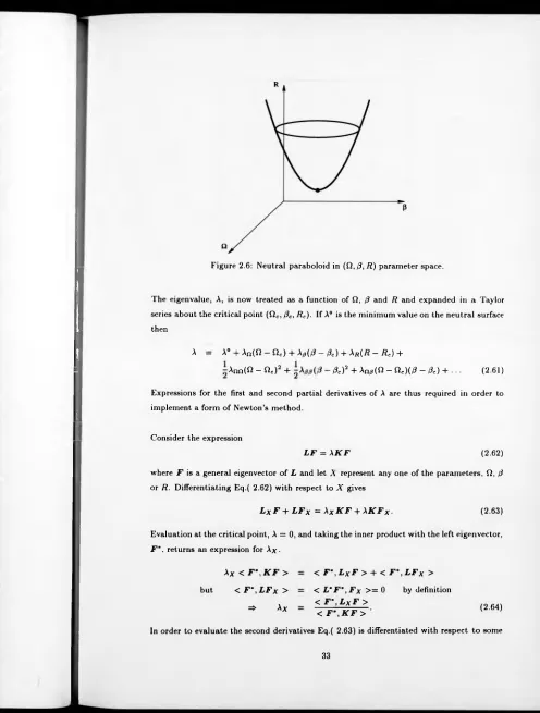
2.6. Neutral paraboloid in (f'l,(3,R) space. 33
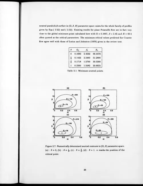
2.7. Calculated neutral contours in (fi, (3) parameter space. 36
2.8. First order solutions for a number of mean states. 41
2.9. Roll cell amplitude as a function of spanwise wavenumber, (3. 44
3.1. Coordinate system and flow configuration. 55
3.2. Temporal and spatial growth rates for rigid wall boundary. 59
3.3. Variation of wavenumber with frequency for the rigid wall. 61
3.4. Rigid wall eigenfunctions at a number of frequencies. 61
3.5. Theoretical plate-spring model for compliant wall. 62
3.6. Free wave solutions for a plate-spring compliant wall. 66
3.7. Reductions in spatial growth rate using optimal wall parameters. 69
3.8. Variation in maximum spatial growth rate with ad. 69
3.9. Amplification rates showing onset of travelling-wave flutter. 73
3.10. Phase speeds for Rayleigh and travelling-wave flutter instabilities. 73
3.11. Complete eigenvalue spectrum for N=48 and 54. 75
3.12. Eigenfunctions for flow-based and wall-based instabilities. 75
3.13. The effect of wall damping at Ck e= 0.2. 78
3.14. The effect of wall damping at Ck e — 0.15. 78
4.1. Falkner-Skan profile for ¡3 = —0.15. 81
4.2. Double layer viscoelastic compliant wall construction. 88
4.3. Comparison of spatial amplification rates with results of Yeo (1988). 96
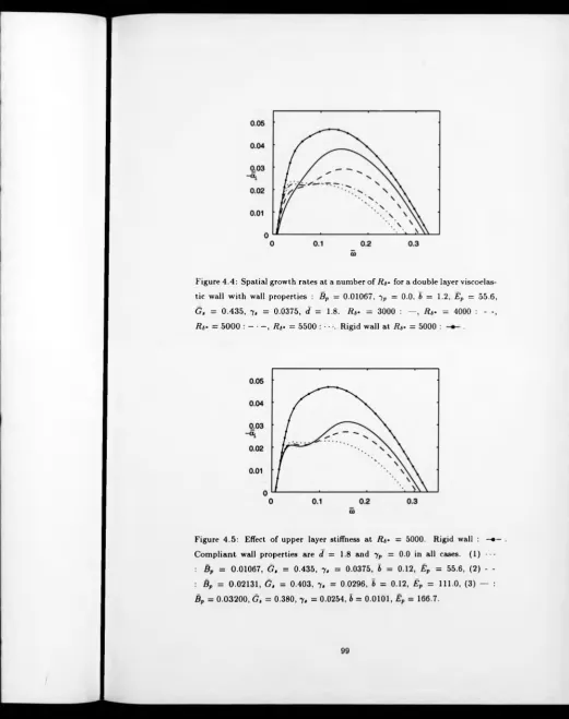
4.4. Spatial growth rates at a number of Reynolds numbers for a double layer
viscoelastic wall. 99
4.6. Effect of upper plate damping on spatial growth rates at Rb = 5000. 100
4.7. Effect of substrate thickness on spatial growth rates at Rb = 5000. 100
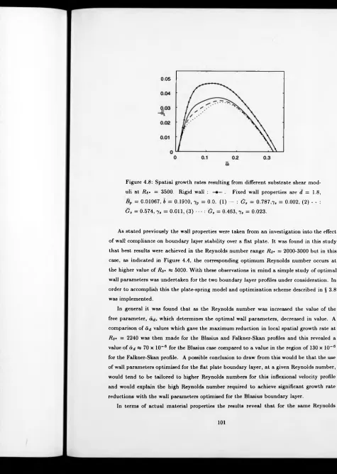
4.8. Spatial growth rates resulting from different substrate shear moduli at
R*6 = 3500. 101
4.9. Eigenfunctions for rigid wall. 104
4.10. Eigenfunctions for compliant wall. 104
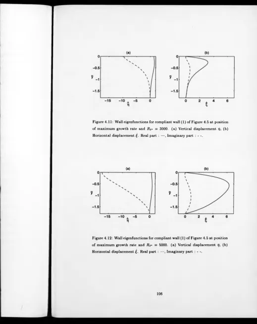
4.11. Wall eigenfunctions at Rb = 3000. 106
4.12. Wall eigenfunctions at Rb = 5000. 106
4.13. Wall displacements for walls of different depths. 107
4.14. Reynolds stress production and viscous dissipation distributions. Ill
4.15. Comparison of pressure work distributions for rigid and compliant walls. Ill 4.16. The effect of wall compliance on numerical values of terms in the energy
equation. 112
6.1. Mean velocity profiles for rotating disc. 134
6.2. Neutral curve for stationary disturbances over rigid boundary. 141
6.3. Free wave solutions for an infinitely deep single-layer viscoelastic wall. 146
6.4. Compliant wall neutral curves for stationary disturbances. 151
6.5. Amplification rates for stationary, Type 1, disturbances as a function of
wavenumber, (3, showing the effect of wall compliance. 153
6.6. Amplification rates for stationary, Type 1, disturbances as a function of
wave angle. 153
6.7. Variation of stationary mode group velocity with Reynolds number and
wall type. 156
6.8. Rigid and compliant wall stationary, Type 1, eigenfunctions at R = 600. 157
6.9. Wall eigenfunctions for Type 1 stationary mode at R = 600. 157
6.10. Amplitude ratios for the Type 1 stationary disturbance. 159
6.11. Amplification rates for stationary, Type 2, disturbances as a function of
wavenumber, (3,showing the effect of wall compliance. 161
6.12. Rigid and compliant wall stationary, Type 2, eigenfunctions at R = 300. 161
6.13. Wall eigenfunctions for Type 2 stationary mode at R = 300. 162
6.14. Comparison of energy terms for rigid and compliant walls at R = 600. 167
6.15. Reynolds stress distributions at R = 600. 167
6.16. Comparison of energy terms for rigid and compliant walls at R = 300. 169
6.18. Representation of geostrophic flow. 171
6.19. Energy budgets for rigid wall Type 1 and 2 disturbances at R = 450. 171
6.20. Vortex structure at R = 600 for stationary Type 1 mode. 172
6.21. Characteristics of the most unstable travelling disturbances as a function of
frequency for R = 300 and R = 400. 175
6.22. The effect of wall compliance on the Type 1 instability across the unstable
frequency range at R = 300. 176
6.23. Travelling disturbance amplification curves at R = 400 for compliant wall. 176 6.24. The effect of wall compliance on amplification rates using the Orr-Sommerfeld
equation. 178
6.25. Minimum Reynolds number for onset of interaction as a function of frequency. 180 6.26. Eigenmode structure and group velocity at R = 369, uj = 0.004 for compliant
wall. 180
6.27. Eigenvalue spectrum in terms of ¡3 for rigid and compliant walls at R = 400. 182 6.28. Eigenvalue spectrum in terms of e and phase speed for rigid and compliant
walls at R = 400. 182
6.29. Flow eigenfunctions at R = 400, uj = 0.004. 184
6.30. Wall eigenfunctions at R = 400, u; = 0.004. 184
6.31. Effect of rotation rate at R = 400, u; = 0.004. 185
6.32. Effect of wall damping at fi = 20rad/s, R = 400, ut = 0.004. 186
6.33. Effect of Reynolds number on amplification rate at uj = 0.004. 186
6.34. Energy budgets for compliant wall at R = 400, uj = 0.004. 190
6.35. Reynolds stress and viscous dissipation distributions for compliant wall
at R = 400 and u> = 0.004. 191
6.31. Effect of degree of wall compliance on energy budgets. 185
6.37. Maximum amplification rate of travelling-wave flutter instability as a function
of frequency. 194
6.38. Eigenfunctions for travelling-wave flutter instability. 195
LIST OF TABLES
2.1. Minimum neutral points for rotating channel flow. 36
2.2. Coefficients of the modulation equation at the minimum critical point for a
number of basic states. 42
3.1. Optimal wall properties defined by the wall parameter â<*. 70
3.2. Variation of phase speed at upper neutral point with wall type. 71
6.1. The effect of wall compliance on the most amplified mode of the Type 1
stationary instability. 156
6.2. Wave angle and value of (3R at position of maximum amplitude ratio. 159
6.3. Data corresponding to maximum growth rate of the Type 1 instability for
travelling disturbances at R = 300. 175
6.4. Variation of propagation angle and group velocity angle across eigenvalue
ACKNOW LEDGEMENTS
This thesis is dedicated to my Mum and Dad whose care and support has always been, and continues to be, of immense encouragement to me and is dearly appreciated.
I would like to thank my supervisor, Professor Peter W. Carpenter, for his guidance and to express my gratitude for his help over the last two years or so. 1 would also like to thank Dr. Tom J. Bridges who supervised my early work at the Mathematics Institute and Dr. Chris Davies for his helpful discussions.
Special thanks must also go to Matthew Keeling whose understanding and reassurance have been so important to me.
DECLARATION
I certify that this thesis is my own composition and that except where specific reference is made is an account of work undertaken by myself. No part of this thesis has been submitted for a degree at any other university.
Some of the work in Chapter 2 has been published in : Bridges, T.J.. and Cooper, A.J., (1995)
“Spanwise Modulation of Streamwise Rolls in Rotating Channel Flow”, Q. J. Mech. Appl. Math., 48, pp. 257-284.
Parts of Chapter 6 appear in :
Cooper, A.J., and Carpenter, P.W., (1995)
SUMMARY
The effects of system rotation and passive wall compliance on hydrodynamic stability is investigated.
Rotating channel flow is studied where a Coriolis force instability mechanism produces streamwise rolls at modest Reynolds numbers and rotation rates. The linear stability of mean flow states consisting of a combination of plane Poiseuille and Couette flows is con sidered using spectral Chebyshev collocation with a staggered grid. A Newton algorithm is implemented in three-dimensional parameter space to calculate minimum points of the neu tral surfaces. Weakly nonlinear behaviour of the rolls is studied using a Ginzburg-Landau formulation and accurate numerical values for the equation coefficients indicate supercritical instability.
Effects of external pressure gradient and three-dimensionality on boundary layer stability over compliant walls is examined. In these cases an inflexion point in the boundary layer profile promotes a powerful inviscid instability mechanism.
Two-dimensional profiles, including a Falkner-Skan representation, are considered in in viscid and viscous analyses with plate-spring and viscoelastic compliant wall models. Walls which are rendered stable with respect to hydroelastic instabilities are shown to reduce maximum spatial growth rates by up to 60%.
CHAPTER 1
IN T R O D U C T IO N .
1.1 General Overview.
The subject of hydrodynamic stability has remained a fundamental area of research in fluid mechanics since the pioneering work of Osborne Reynolds over a century ago. The tendency for laminar flows to become unstable leading to a turbulent state was first demonstrated by Reynolds' experiments in 1883 and this phenomenon continues to provide an important area of interest because of the implications of this in many real situations and engineering applications. As a whole the subject of hydrodynamic stability can cross over many scien tific fields from engineering, meteorology and oceanography to more applied areas such as astrophysics and geophysics. Theoretical studies have always been hindered by the nonlinear nature of the governing stability equations and thus stability analyses have relied heavily on simplified problems and the use of linearised theory. The advancement of computing capabilities and the introduction of new mathematical techniques aimed at extracting some of the nonlinear characteristics now allows more complex stability problems to be analysed.
The way in which laminar flow becomes unstable and what determines when the transi tion process occurs are both dependent on flow configuration and external influences such as buoyancy effects brought about by fluids of variable density, magnetohydrodynamic forces, external pressure gradients and centrifugal and Coriolis effects brought about by system rotation. Laminar-turbulent transition is generally initiated by some change in the bal ance of forces within the flow system which acts to alter the flow structure. In boundary layer or plane channel flows, for example, instability first appears when travelling Tollmien- Schlichting (T-S) waves become amplified. When this occurs depends on certain parameters of the flow, characterised by the Reynolds number. For example, in the above two cases when the Reynolds number is raised above a critical value the driving pressure forces cease to be balanced by forces which are inertial and viscous in nature and amplification of dis turbances in the flow are brought about. In general viscosity has a stabilising influence on a flow because of its ability to dissipate disturbance energy so only when viscosity is taken below some level will the equilibrium of forces be unbalanced.
a different form to that of the propagating T-S waves. The appearance of stationary roll cells is the result of the departure from the laminar state when a fluid layer between two plates is heated from below. In this case density divisions instigate the onset of the instability. These roll cells also develop in geophysical flows where body forces govern the transition process and of particular importance in the formation of these roll cells are body forces arising as a result of system rotation. An imbalance between centrifugal force on the fluid particles and the local pressure gradient is responsible for the centrifugal instability observed in cylin drical Couette flow. When the angular velocity of the inner cylinder exceeds some critical value so-called Taylor vortices are generated which occur periodically in the axial direction and in this case each close to form a toroidal shape. The vortex structure then undergoes a series of secondary-type instabilities as the rotation speed is increased leading ultimately to a turbulent state. This type of phenomenon is also apparent for flows in curved channels and over concave walls. Roll cells can also develop as a result of a Coriolis force mechanism acting on flow systems and is a route to transition in shear flows.
Negative pressure gradients have a destabilising influence because adverse pressure gra dients generate points of inflexion in the associated velocity profiles which is a condition originally shown by Rayleigh (1880) to give rise to an inviscid instability mechanism. This in turn generally leads to powerful instabilities.
Areas of commercial interest as far as stabilising flows is concerned lie in reducing drag over surfaces. In essence if the flow can be stabilised by external factors, such that the result is the maintenance of laminar flow over a greater part of the surface, then the drag reductions on bodies moving in a fluid achieved by this could be exploited to gain greater speeds/fuel efficiency. This process is generally known as laminar flow control and various methods have been used in attempts to achieve this. For application in air suction techniques have been applied both in theory and practise with theoretical results indicating the potential for this method as a means of laminar flow control but problems in practise have limited full-scale implementation of such a method. More recently wall compliance or boundary flexibility has been shown to be effective in postponing the laminar-turbulent transition process in marine applications.
1 .2 M otivation.
cur-rent work is then two-fold.
1.2 .1 The Effects of Rotation on Plane Channel Flow.
In the first case the effect of rotation on a well-known flow configuration is assessed where the influence of rotation is studied through the action of Coriolis forces rather than centrifu gal influences. The centrifugal instability mechanism has received a considerable amount of attention, for example in the classical Taylor-Couette concentric cylinder problem, and has lead to a substantial understanding of the transition process in geometries affected by this mechanism. However, the Coriolis force instability mechanism which generates the roll-cell form of primary instability has received comparatively less consideration. A particular ex ample of the effects of Coriolis forces on shear flow is that of a flow in plane channel subject to rotation about some spanwise axis. Over the past twenty years or so this problem has begun to attract more interest both theoretically and experimentally.
The work of Benton (1956) on the rotation of pipe flow was perhaps the first to give evidence of longitudinal roll cells, but it was not until Halleen and Johnston (1967) and Hart (1972) that experiments were undertaken on the rotating channel. Hart had recognised that the majority of experiments concerning rotating fluids had, up to that date, tended to concentrate on cylindrical systems. As well as focusing only on the centrifugal instability mechanism these experiments were designed for operation under high rates of rotation. A feature of the Coriolis force instability, which occurs in rotating channel flow, is the onset of streamwise roll cells at much lower rotation rates and Reynolds numbers than other unstable flows. For example, T-S waves in a plane channel become amplified at a Reynolds number almost two orders of magnitude higher than that required for the onset of roll cells when the system is subjected to spanwise rotation. This indicates the comparative strength of the Coriolis force instability mechanism. Further experimental investigations have been carried out more recently by Alfredsson and Persson (1989) who provide results in part through the use of flow visualisations. New work by Marliani et al. (1994) has sought to consider the effects of moderate acceleration and deceleration on rotating channel flow.
however, is mainly on the laminar flow case but some turbulent flow results will be discussed.
The instabilities which arise when a plane channel is subjected to rotation about a spanwise axis differ in a number of ways to the same flow situation in the absence of rotation. Knowledge about the behaviour of these roll cells is of fundamental importance in leading to a greater understanding of the physics of transition in shear flows. A number of such flows can be established within the channel geometry, the most widely studied being that of plane Poiseuille which possesses the characteristic parabolic streamwise velocity profile. Attent ion here will focus on a wider family of basic profiles which interpolates between plane Poiseuille flow and plane Couette flow which is linearly stable in the absence of rotation. This problem is also amenable to investigation of the role of nonlinear stability of the flow where previously the Stuart-Landau expansion or weakly nonlinear theory has been used to consider the nature of the bifurcation to streamwise rolls with Finlay (1989), Ng et al. ( 1990) and Singer (1992) establishing supercritical bifurcation to rolls in rotating Poiseuille flow which effectively means the roll cells settle down to form a new laminar flow. A variation on this method will be made through the derivation of a Ginzburg-Landau equation. This was originally derived by Newell and Whitehead (1969) when considering the stability problem of Bénard convection but has not commonly been used in the present context. One advantage of using this sort of equation rather than the standard weakly nonlinear theory is that the stability of the rolls to spanwise modulation may be considered. This type of instability, known as Eckhaus instability, can become significant in problems with large aspect ratio.
Exploring the instability characteristics in this geometry would be of interest in applica tion to devices involving rotating fluids. Examples often cited are flows in turbine blades, inside impellers of centrifugal pumps and certain geophysical flows.
1 .2 .2 The Effects of Wall Compliance on Boundary Layer Stability.
The second case of interest is that of controlling laminar-turbulent transition through the use of wall compliance in an area that has to date been left largely unexplored. This in volves applying existing knowledge on the effects of wall compliance to instabilities which are inviscid in nature rather than the T-S instability where results are well documented.
applications. The skin friction drag reducing capabilities of compliant walls suggests in creased vessel speeds and greater energy efficiency could be possible. The maintenance of laminar flow over a body is also known to greatly reduce the degree of noise it produces which would give submerged bodies an increased transparency to detection. Compliant walls could therefore also be useful as an acoustic application.
The original work in this novel field of laminar flow control was undertaken by Kramer (1960) under the inspiration of the phenomenal swimming speeds attained by dolphins after Gray (1936), from a purely observational point of view, first brought this subject to the attention of the scientific community. Kramer investigated the structure of the dolphin skin and developed several prototype coatings designed to simulate the skin properties. Testing was performed by measuring the drag on solid bodies covered with coatings of different material specification. Significant reductions in drag were recorded and Kramer implied this was possible as a result of distributed damping. In other words, the inclusion of a highly viscous fluid within the wall was thought to damp out the fluid instabilities which initiate the transition process.
Early theoretical work to follow was that of Benjamin (1960,1963) and Landahl (1962). This research supported the case for achieving drag reduction through the use of compliant walls but at the same time indicated the possibility of additional wall-based modes of in stability absent in the case of rigid boundaries. Contrary to Kramer's theory on the control mechanism the work of Benjamin showed that wall damping actually destabilised T-S waves. Damping in the original walls was probably successful in suppressing wall-based instabilities rather than reducing the growth rates of the flow-based instabilities as first suggested by- Kramer. Despite its apparent success Kramer's work was thrown heavily into doubt on the grounds of subsequent experimental research where verification of results was sought but no corroborative evidence was ever achieved.
Arora (1988) and Yeo (1988) who modelled wall compliance with multiple layers of viscoelas tic material. A breakthrough in carefully controlled experiments was made by Gaster (1987) and Daniel et al. (1987) who assessed the effects of wall compliance on Tollmien-Schlichting (T-S) waves in flat plate boundary layers. Results confirmed that wall compliance could have a significant stabilising influence on the T-S waves thus effectively leading to a delay in the onset of transition. Comprehensive reviews of the work have been made by Riley et al. (1988), where the emphasis is on experimental work, Gad-el-Hak (1986) and Carpen ter (1990). More recent work by Dixon el al. (1994), not included in the aforementioned publications, has conservatively indicated six fold increases in transitional Reynolds number using specifically optimised compliant walls.
Most of the preceding research has concentrated on the effects of wall compliance in relation to the two-dimensional flat plate boundary layer with zero external pressure gradi ent. In this case the boundary layer disturbances take the form of T-S waves which become destabilised by an essentially viscous mechanism. Wall compliance basically controls this type of instability by reducing the rate of production of disturbance kinetic energy by the Reynolds stress, by increasing the viscous dissipation and bringing in additional energy dis sipation mechanisms. The effect of a compliant boundary therefore alters the ratio between energy production and dissipation allowing the growth of boundary layer disturbances to be suppressed.
In real aerospace and marine applications, however, boundary layers are usually three- dimensional and/or develop in a non-zero pressure gradient which is likely to be adverse over some part of the surface. The effects of external pressure gradient and three-dimensionality of the boundary layer on compliant wall performance has remained largely unexamined. If wall compliance is ever to be viable as a practical means of maintaining laminar flow’ then its performance under these conditions must be critically assessed.
ber with amplification rates considerably higher than those of the T-S instability and the transition region is typically shortened in two-dimensional flows by the presence of an ad verse pressure gradient. It therefore needs to be established whether passive wall compliance is capable of controlling disturbance growth to a sufficient extent when this inflexion point instability dominates.
Three-dimensional flows of research interest include boundary layers which develop over sweptback wings, rotating cones and rotating discs as well as those specific to other aerospace and marine applications. Fully three-dimensional boundary layers are susceptible to a form of instability known as crossflow instability which invariably dominates the breakdown of laminar flow. This form of instability is common only to three-dimensional boundary layers and is a route to transition in the leading edge region of swept wings. A characteristic feat ure associated with the crossflow phenomenon is the presence of a velocity component within the boundary layer which exhibits a point of inflexion which then promotes an instability mechanism dominated by inviscid effects somewhat analogous to the Rayleigh instability of two-dimensional flow’s.
Discovery of the crossflow instability is attributed to Gray (1952) who observed, whilst studying the flow over sweptback wings, uniformly spaced vortices stationary with respect to the wing body prior to the onset of transition. This structure was absent over unsw-ept wings where the flow is two-dimensional. An independent study by Owen and Randall (1952) interpreted these observations as the now termed crossflow phenomenon.
transition process.
The rotating disc boundary layer has long been use as a model problem for studying three-dimensional boundary layers since it exhibits so many of the features commonly found in more complex three-dimensional cases. It is particularly amenable to theoretical studies in view of the exact similarity solution of von Karman (1921) to the Navier-Stokes equations for the mean flow field. The boundary layer is also of constant thickness so no assumptions about boundary layer growth have to be made. Experimentally the problem provides a relatively convenient and compact form. The effects of wall compliance on instability in three-dimensional boundary layers can therefore be investigated by considering this simpler model problem. However, despite the apparent simplicity of the flow field the instabilities which arise for a rigid boundary are considerably complex and have received substantial attention in their own right. Before wall compliance is introduced the form of the instabilities in this problem need to be clearly established. This is accomplished in part by a review of work to date on this subject.
1 .3 Outline of Contents.
Following this brief introduction to the contents of this study each major section will be preceded by a review of literature relevant to the particular problem in question.
Chapter 2 provides the background required for the rotating channel problem. Aspects of
both linear and weakly nonlinear theories are considered in relation to the rotating channel stability problem for a number of different mean shear flows established within the chan nel. Neutral stability curves and Ginzburg-Landau coefficients are used to establish stability characteristics for the family of mean flow fields.
Chapter 3 introduces the terminology essential to the study of problems involving wall
compliance. Classification of instabilities is discussed, as are the types of instability which can arise as a direct result of wall compliance. A two-dimensional boundary layer which de velops in the presence of an adverse pressure gradient and how the stability characteristics of this type of flow are affected by a compliant boundary is then investigated through the use of a plate-spring wall model and inviscid analysis.
Chapter 4 extends the work of the preceding chapter through the inclusion of viscous ef
Chapter 5 describes the differences which arise in the stability analysis of a three-dimensional
boundary layer and how standard techniques are adapted to accommodate the additional dimension. This is followed by a review of work concerning the stability of the boundary layer which develops over a rotating disc.
Chapter 6 contains work concerning the rotating disc/compliant boundary problem focus
ing on a single-layer viscoelastic wall model. This chapter divides into three main areas which involve the analysis of stationary disturbances, travelling disturbances and the gen eration of hydroelastic instabilities in this flow geometry.
Chapter 7 draws general conclusions from this study and suggests possible areas of interest
CHAPTER 2
ST A B IL IT Y O F R O T A T IN G
C H A N N E L FL O W .
2.1 Introduction.
The aim of this section of work is to study the primary instability of spanwise periodic streamwise roll cells which occurs when plane channel flow is subjected to some constant spanwise rotation and in addition to the often studied plane Poiseuille mean flow a number of other basic states are considered. A general basic state is thus defined through the use of an interpolation parameter to provide a continuous family of mean velocity profiles. Linear stability analysis is first employed in order to determine whether the qualitative effects of rotation on the system remain essentially the same for all the shear flows investigated or whether some different characteristics arise.
With the introduction of rotation the stability characteristics become dependent on two parameters, the Reynolds number and rotation number (or dimensionless rotation rate) which define a neutral surface or paraboloid rather than the usual two-dimensional parabolic neutral curve of the non-rotating case. A Newton algorithm is used to determine accurately numerical values for the minimum point of the corresponding neutral surfaces in the full three-dimensional parameter space. This improves upon existing results where calculations have been confined to a restricted parameter space at fixed rotation rates. Consideration of such a two-dimensional section of the neutral surface means the rotation rate must be carefully selected if the true global minimum value is to be located.
A weakly nonlinear analysis is then applied in order to study the spanwise modula tion of the streamwise rolls leading to the derivation of a Ginzburg-Landau equation. The coefficients of this equation are determined numerically in order to establish whether the bifurcation to rolls is supercritical or subcritical for the whole family of states investigated. However it must be recognised that supercritical bifurcation does not satisfactorily establish that the roll cells are stable to spanwise modulations since in large aspect ratio systems, the possibility of an Eckhaus-type instability arises.
for a number of different rotation rates and for a number of basic flow fields. The eigenvalue problem which results from this analysis is solved numerically using a spectral collocation method with a staggered grid. Minimum critical points are determined numerically and used in the subsequent calculation of the Ginzburg-Landau coefficients of the modulation equation.
2 .2 Review of Theoretical and Experimental Works.
A brief outline of the original and main contributors to work in this field was made in Chap ter 1 but this is now expanded upon in more detail.
A good description of the Coriolis force instability mechanism appears in Alfredsson and Persson (1989) where it is stated that a direct result of channel rotation about some spanwise axis normal to the streamwise flow direction is a Coriolis acceleration, SV A U , where SI' is the rotation vector and U the basic flow vector. This would give rise to a force normal to the channel walls and acts towards the channel leading edge. For the case of a parabolic mean flow profile the largest force occurs at the centre of the channel causing the leading side of the channel to be destabilised and the trailing side stabilised. Two parameters are thus needed to characterise the flow, the Reynolds number, R = U0h/v and the rotation number, Q = Q"h/U0 (the inverse of the Rossby number, R0) where U0 is the maximum velocity of the mean flow, h the channel half width and $1“ the dimensional rotation rate. Definitions of these parameters vary in the published work but whenever comparisons are made appropriate scalings have been implemented.
Tritton and Davies (1985) also give a description of the instability mechanism in terms of a “displaced particle” argument.
the flow to be fully developed within the interior of the channel, making end effects negligible. The channel is mounted on a rotating table and the flow is driven by generating a constant pressure gradient across a chimney at each end of the channel.
The different stages of transition show up well in the flow visualisation studies of Al- fredsson and Persson (1989) who add further observations to those of Hart. These flow visualisations were made through the introduction of titanium-dioxide coated platelets into the fluid which when illuminated show stream surfaces. In particular the roll cells show up as alternating bright and dark bands when viewed in the rotating frame. Alfredsson and Persson describe a secondary instability in evidence at higher Reynolds numbers which is seen as a twisting of the roll cells and if rotation is increased further at this stage a wavy disturbance arises and moves in the upstream direction. Both twisting and waviness is seen to originate at the downstream end of the channel. This type of secondary instability has also been found numerically by Finlay (1990) where it is described as being similar to the twisting of Dean vortices which can arise in curved channel flows and the numerical simulations of Yang and Kim (1991) have also been able to reproduce the wavy vortices observed in experiments. Turbulence develops with a further increase in rotation although some embedded roll cells still appear to be in existence. Another observation made from these experimental investigations was the possible splitting of the flow visualisation streaks at some downstream location. At this stage, however, it was unclear as to whether this was a manifestation of the flow visualisation technique or whether actual splitting of the streaks (implying a splitting of roll cells) was occurring. It was not until the work of Guo and Finlay (1991) that some reasoning behind these observations was formed. The theories developed in this case were based on consideration of Eckhaus-type instabilities which become important in large aspect ratio experiments and will be discussed later.
As well as some of the original experimental work Hart (1972) also considered the rotat ing channel problem theoretically. Within this study it was shown that the stability problem is directly analogous to the instability of a fluid between two plates which are heated differ entially and using this analogy a necessary condition for roll cell formation was formulated and defined as QUy > 5, where Uy is the gradient of the mean flow velocity. (This condition states that the total vorticity must be negative and comes from the requirement of a negative thermal gradient in the analogous problem.) This was applied to rotating Couette flow and Poiseuille flow to predict dividing regions for stability and instability (based on rotation rate and ratio of rotation rate to critical Reynolds number).
range 0 < $2 < g with critical parameters 0C = 1.55 and Rc = 20.65 at Cl = 0.25 where /? is the spanwise wavenumber. These values were predicted from the critical Rayleigh number in the analogous problem and in analogy with the small gap rotating cylindrical problem was used to determine stability characteristics for rotating plane Poiseuille flow. Using the critical Taylor number in this case determined Re = 66.4 at Q = 0.1667. Symmetry of the basic profile in this case results in instability in the rotation range 0 < il < 1 for rotation in either direction. The values of these critical parameters have been repeated in a number of subsequent numerical calculations. However, a criticism of these results is that they are not actually calculated in the full three-dimensional parameter space and it may be possible that truly global minimum critical values have not been identified.
Linear stability theory limits the analysis of this problem to determining critical values and local amplification rates or neutral curves and in order to study more fully the instability of the roll cells weakly nonlinear theories, secondary stability analyses and full numerical simulations have been conducted. Finlay (1989), Ng ti at. (1990) and Singer (1992) apply the Stuart-Landau theory to rotating plane Poiseuille flow all determining supercritical bifurcation to streamwise roll cells.
The flow visualisation experiments of Alfredsson and Persson (1989) indicated high am plification rates such that the amplitude of the roll cells may grow large enough to become unstable to oblique disturbances. Ng et al. undertake a secondary stability analysis at the parameter values for which Alfredsson and Persson made these observations (R = 382, il = 0.028, spanwise wavenumber 0 = 3.0) and their theory indicated two ranges of stream- wise wavenumber over which secondary instability exists. Alfredsson and Persson proposed a theory for the occurrence of this secondary instability based on the assumption that it arises as a result of the development of a point of inflexion in the basic velocity profile. This was subsequently discounted, however, following the calculation of only stable eigenvalues for a purely streamwise disturbance on an inflexional basic flow and all disturbance components were found to be required for this secondary instability to occur.
stabilisation to the Taylor-Proudman regime. The full nonlinear time-dependent Navier- Stokes equations are solved by finite difference techniques with the inclusion of end effects making it a particularly good comparison with experimental situations. For a channel of aspect ratio 8 and in the parameter range 0 < R < 375, 1.66 x 10⁻⁵ < Q < 1 the following results are typical. The secondary flow, originally seen in the experiments of Hart, forms as two single vortices, one compressed against each end of the channel wall, with a length scale of the same order as the channel width. The development of this double-vortex structure into fully streamwise roll cells with increasing rotation rate is then calculated. Through the simulations (using a time-marching scheme) this is seen as a stretching of the double-vortex structure which eventually leads to the formation of an even number of counter-rotating vortices where the actual number of vortex pairs is dependent on the aspect ratio of the system. Finally, moving to higher rotation rates the roll cell vortices break down and restabilise to a Taylor-Proudman regime seen as a double-vortex structure similar to the secondary flow phenomenon but stretching further into the interior of the channel.
As mentioned earlier the numerical simulations of Finlay (1990) revealed the wavy-type of secondary instability that has been observed experimentally. Three-dimensional spectral simulations using the time-dependent, Navier-Stokes equations reveal two types of wavy vortex flows named WVF1 and WVF2 by Finlay. WVF2 was found to occur only at low rotation rates and to have much lower amplification rates than the WVF1 structure whereas the WVF1 was found to develop at all rotation rates considered and is most likely to be the experimentally observed structure owing to the higher growth rates associated with it.
The weakly nonlinear analyses leading to prediction of supercritical bifurcation to rolls (Finlay, 1989, Ng et a/., 1990, Singer, 1992) is not strictly sufficient for roll cell stability when considering large aspect ratio systems. The Eckhaus instability becomes important in such cases and has been shown to be present in Taylor-Couette systems (Dominguez-Lerma et al., 1986). The Eckhaus instability arises from the consideration of roll cells subjected to two-dimensional spanwise perturbations. At the critical point, predicted from linear stability theory, the critical and only wavenumber for the roll cells is /?c. As R is increased above Rc a band of wavenumbers which will give stable roll cells is expected. The width of this band is determined by the Eckhaus instability boundary where the two-dimensional vortices with wavenumbers within this boundary are stable with respect to perturbations. The original criterion, put forward by Eckhaus (1965), for the stable wavenumber band of T-S waves is
f t- /? - < 0 - Pc <0+ -P ' v/3
and Taylor-Couette problems. Eckhaus stable bands of wavenumbers have been found in these cases and the latter shown to have an Eckhaus boundary which is open ended and of the same form as the primary instability neutral curve and lies within the linearly unstable region. Guo and Finlay (1991) have analysed the rotating/curved channel system and found the Eckhaus boundary in this case to be a small closed region tangential to the critical point of the primary instability neutral curve. Outside this boundary splitting or merging of vortex pairs is predicted to be possible which lends support to the experimental observat ions of Alfredsson and Persson (1989). Wavenumbers selected by the Eckhaus instability appear to determine which process occurs. For small wavenumbers it is predicted that two vortex pairs can be split by a new pair to form three pairs, or if the wavenumber is large two vortex pairs will merge. Selection of spanwise wavenumbers is made by the Eckhaus instability for moderate Reynolds numbers and wavenumbers least unstable to spanwise perturbations appear to correspond to those observed experimentally.
Of note in this problem is the finding that the Eckhaus criterion is violated even for R close to Rc in some cases. A possible reason for this put forward by Guo and Finlay focuses on the differences in the basic flow between plane Poiseuille flow and the Taylor-Couette problem where the Eckhaus criterion is satisfied. In the latter case the velocity in the stream wise direction takes its maximum value at the wall whereas the maximum occurs in the centre of the channel for plane Poiseuille flow. This theory can be followed up by considering a family of basic states for the rotating channel problem which interpolates between rotating plane Poiseuille flow and Couette flow. Varying the interpolation parameter is effectively equivalent to moving the point of maximum streamwise velocity from the channel centre to the wall.
Many of the features associated with rotating channel flow and in particular the ap pearance of roll cells above critical parameter values are similar to occurrences in curved channel flow. In this configuration so-called Dean vortices can arise as a result of a centrifu gal instability mechanism. Matsson and Alfredsson (1990) consider the combined effects of rotation and curvature on channel flow and this study reveals that compared to when there is just channel curvature the introduction of rotation can stabilise the flow if the centrifugal and Coriolis effects are counteractive. A particularly strong secondary instability found in curved channel flow was found to be completely removed if rotation was introduced in the right sense.
in boundary layer flows but not in flow configurations where body forces are influential. The aim in this work was to consider non-parallel effects in the rotating channel problem with one example of direct practical relevance to this being the consideration of the effects of changes in cross-section of cooling passages of turbine blades. The apparatus for this investigation consisted of the usual channel mounted on a rotating table where acceleration or deceleration of the flow was made possible through the inclusion of wedge shaped end plates with the wedge angle determining the degree of acceleration or deceleration in the system. Experiments were performed keeping the flow rate (or Reynolds number) constant and increasing the rate of rotation. Flow visualisations for a parallel channel showed the longitudinal vortices as streaks occupying the whole space of the channel whereas for both accelerated and decelerated flows the streaks only occupied parts of the channel implying the simultaneous presence of both the roll cell state and the one-dimensional state. For the case of decelerated flow longitudinal vortices were in evidence at the entrance to the channel and disappeared as progression was made downstream. The opposite was true for the accelerated flow where the streaks were more pronounced at the downstream end of the channel. These observations are probably due to the influence of the flow rate on the production of roll cells since flow rate is directly related to the Reynolds number and if the acceleration or deceleration of the flow is enough to take flow parameters above or below the critical values required for the onset of the roll cells then this would explain the different structures observed along the channel length.
The effect of rotation on fully turbulent flow has many implications in real systems such as oceanic and atmospheric flows as well as engineering applications where rot ation is a significant factor. Early experiment al work to investigate the effects of Coriolis force on fully developed turbulent flow was performed by Johnston el al. (1972). Throughout references to stablisation/destabilisation of turbulent flow should be viewed in a slightly different context to that associated with laminar flow and are interpreted as a reduction/increase in turbulence intensity.
One of the features revealed in the study by Johnston el al. was that small rot at ions lead to the mean turbulent velocity profile taking on an asymmetric shape as a direct result of the Coriolis force action. At high rotation rates local production of turbulence was found to be eliminated in the low pressure wall region and the formation of a laminar wall layer was observed. Conversely, the turbulent flow was augmented at the high pressure wall resulting in a destabilised region and at this channel side a Taylor-Gortler vortex type structure was observed embedded within the turbulent flow.
the use of a two-layer model. Integrated averages of eddy viscosity were used to represent turbulence stress levels and numerical results were able to predict the onset of the vortex instability above fl ss 0.00667 for the Reynolds number range 4500-26250 and were in good agreement with experimentally determined conditions for this instability. More recently Kristofferson and Andersson (1993) have performed direct numerical simulations for fully developed turbulent channel flow, subjected to this spanwise rotation, using finite difference techniques to solve the governing equations. These calculations confirm earlier results and give some additional features. For weak rotations (il = 0.00333) the turbulent flow structure was found to change only slightly but the first signs of the rotation influence were revealed as opposing effects at each channel side with these differences becoming more prominent as the rotation rate is increased. Turbulence levels become greater at the high pressure side and decrease in intensity at the opposite side verifying the observations of Lezius and Johnston. This then results in the asymmetric appearance of the mean velocity and Reynolds stress profiles. At a value of Q = 0.1667 the total elimination of turbulence intensity is predicted at the stabilised side of the channel. The streamwise Taylor-Gortler vortex state arising as a direct result of system rotation is simulated well in these calculations and it was demon strated that these counter-rotating vortices tend to migrate towards the high pressure wall and increase in number as the rotation rate is increased.
2 .3 Channel G eom etry and Governing Equations.
Consider a parallel-walled channel extending infinitely in the streamwise, x, and spanwise, z, directions with walls located at y = =t/i which is subjected to rotation about the spanwise axis at a constant dimensional rotation rate, il*. The geometry and coordinate system are shown in Figure 2.1.
The motion of the fluid passing through the channel is governed by the Navier-Stokes
pressibility. For clarity these equations are written in the rotating frame so that the velocity vector u* and pressure p* in that frame satisfy
and a centripetal acceleration, i7* A(U" A ** ). However, a modified pressure, pm, can be defined which incorporates this centripetal term by using the following vector relation.
y
/ / / / / / / / / / / / / / / / / /
x
/ / / / / / /
[image:33.553.21.527.7.690.2]z
Figure 2.1: Geometry and coordinate system for rotating channel.
equations together with the continuity equation which enforces the condition of fluid
incom-V • um = 0 (2.2)
where x* is the dimensional position vector and /?* = [0,0,fi*]T. p is the fluid density and v the kinematic viscosity.
The extra terms arising as a result of the rotation are a Coriolis acceleration, i2 A u* ,
« • A ( / r A x ') = A**)2]
The pressure can then be redefined as
Pm = P - A * ' ) 2 .
Henceforth the subscript on pm will be dropped and any further expressions involving p will refer to the modified pressure. Using this expression and non-dimension&lising Eqs.( 2.1) and ( 2.2) results in the following non-dimensional governing equations.
^ + (u • V)u + 2/7 A u +Vp — V2u = 0at H (2.3)
<1 S II o (2.4)
Velocities are scaled with respect to a fixed characteristic value, U0, taken in this case to be the maximum value across the channel and lengths are non-dimensionalised by the channel half-width, h. This defines the two parameters which characterise the stability features for this problem, namely the Reynolds number
R = Uoh/v. (2.5)
and the rotation number
n = n mh/u0. (2.6)
For plane Poiseuille flow boundary conditions arise from the requirement of zero velocity at the walls. If u = w]T then
u. = v = w = 0 at y = ±1. (2.7)
The full nonlinear problem described by Eqs. ( 2.3), ( 2.4) and ( 2.7) has an
which defines the mean state and is given by the following flow field. exact solution
u(x,y,z,t) = U(y)= l - (2.8)
t>(*,»,*,«) = o (2.9)
w(x,y,z,t) = 0
p(x, y, z,t) - P(x,y) = - ^ x - 2iiy + + Pa
2 .4 Linear Stability Analysis.
In order to establish some stability characteristics of the flow problem a space and time- dependent perturbation field, s[u', v', u>',p'], is imposed on the basic flow field where e is an arbitrary constant introduced to represent small perturbations or infinitesimal disturbances.
u(x,y, z,t) = U(y) + eu'(x,y,z,t) (2.12)
v(x,y,z,t) = ev'(x,y,z,t) (2.13)
w(x,y,z,t) = ew'(x, y, z,t) (2.14)
p(x,y,z,t) = P(x,y) + sp'(x,y,z,t) (2.15)
The linear stability of the basic flow field is determined by substituting the above expres sions into the governing equations and linearising with respect to the perturbation quantities about the basic state (i.e. terms of 0(e2) and smaller are neglected). This yields the follow ing system of linear equations.
du' du' , dp' , 1 „•> ,
— + t/ — + Uyv' + - 2Qv' - —Wdt dx
dv dP'dx R 1 ,
« + I ' £ + f +2n”' - i v V
dw' ,.dw' dp' 1 9 /
dt * dx dz R
du' dv' dw' _
dx + dy + dz where Uwm % ,
with boundary conditions
u' = v' = w' = 0 at y = ± 1.
(2.16) (2.17) (2.18) (2.19)
(2.2 0) These linearised equations are only valid for infinitesimal perturbations and results should be interpreted in accordance with this. Stability criteria determined using this method do not indicate stability of the basic flow with respect to finite disturbances for which the non linear terms considered negligible here must be included.
The perturbation quantities can either be modelled as spatially or temporally developing disturbances. The spatial theory, first proposed by Caster (1962), is the more physically realistic of the two in most cases when the instability is described as convective, but for neutrally stable disturbances the two forms are equivalent. Since the main purpose of this linear stability analysis is to determine neutral boundaries the perturbation field is assumed to be composed of an exponential time component, therefore developing temporally, with
amplitude functions dependent on the spatial variables such that
[u', u', w', p']T = eA<[ù(i, y, z), v(x, y, i), w(x, y, z),p{x, y, ;)]r + c.c. (2.21 ) where A = Ar + ¿A, is complex valued with the real part of A (or Ar) giving the temporal growth rate.
Substitution of this form for the perturbation components into Eqs.( 2.16)-( 2.18) removes time derivatives to leave
perturbations grow exponentially in time, i.e. Ar > 0, and stable if Ar < 0.
The system of stability equations can be rearranged into a matrix form to define an eigenvalue problem for A as follows.
where V = [ù, v, w, p]T. Therefore, for given values of Q and R, non-trivial solutions are determined by requiring that det(L) = 0.
A number of numerical techniques can be employed to solve this type of eigenvalue problem and the particular method of spectral collocation is employed here. The following section introduces this numerical technique and moves on to describe its application with respect to this specific problem.
2 .5 Numerical M ethod - Spectral Techniques.
Spectral methods are one means of determining numerical solutions to differential equations through discretisation. The foundations of this particular technique are based on the finite series expansion of the solution in terms of some orthogonal expansion functions. The type (2.24) (2.25)
(2.22)
(2.23)
with
û = h = w = 0 at y = ± 1. (2.26)
For fixed values of if and R the basic flow is then deemed to be linearly unstable if the
of expansion functions used gives the main difference between spectral and finite-element methods. In the spectral formulation the functions are global whereas the subdivision of the computational domain involved in the finite-element technique means the functions used are local to each subdomain. Spectral techniques are inherently accurate and generally if the appropriate type of method is used to suit the problem they are computationally efficient methods of solution.
Within the overall framework of spectral techniques there are a number of different schemes, namely Galerkin, collocation and tau which differ in the way the problems are required to be satisfied. A requisite condition in all cases is that the residual, or difference in the differential equation given by the series solution and the actual solution, be minimised. The collocation technique which will be used here tends to be the simplest of the three methods to implement and describes the problem in terms of the discretised solution. The criterion for a satisfactory solution in this case is that the differential equation be satisfied exactly at a number of discrete points known as collocation points.
As well as the different types of method used to formulate the problem there are also a number of choices for the expansion functions used to construct the solution. The most commonly used are trigonometric, Chebyshev and Legendre polynomials chosen appropriate to the particular problem since optimum accuracy is dependent on the selected expansion functions. For example, in a problem which exhibits periodicity the Fourier series expansion would be the most suitable choice, but Chebyshev polynomials prove to be adaptable to a number of different problems and are much more versatile. In numerical studies of instability in plane Poiseuille flow Orszag (1971) has demonstrated that Chebyshev polynomials are better adapted than other orthogonal functions for hydrodynamic stability problems and also lead to more efficient calculations and storage than finite-element techniques. Orszag has also recommended the use of these polynomials because of the rapid decrease in truncation error as the number of polynomials used in the series expansion increases.
The following section describes spectral collocation method using Chebyshev polynomials as the expansion polynomials.
2 .5.1 Chebyshev Collocation.
Chebyshev polynomials are defined on the interval [-1,1] by
T„(;r) = cosn0 where 9 = cos_1(ar), n = 0,1,2,... (2.28)
of these polynomials up to some value N.
N
</<(*) = n=0 (2-29>
In order to implement the collocation method distinct points, Xj, in the domain [-1,1] must be defined with the number of points required being equal to the order of the approximating polynomial expansion. The usual choice for the Chebyshev collocation technique are the Gauss-Lobatto points defined as follows.
X j = cos ^ j = 0 ,..., N (2.30)
These are not evenly distributed across the interval but are more closely spaced at the interval ends and this concentration of points near the boundaries generally leads to more accurate results since in fluid problems this is the region where the most significant effects occur. As such this is also a more economical distribution since if the points were evenly spaced a greater number would be required to give sufficient resolution near the boundaries and the same degree of accuracy in the solution.
Once the collocation points have been defined the solution is evaluated at each of these
locations. N N
= V’(X j ) = a n T n ( X j) = COS ~ N ~ <2 '3 1 )
n=0 n=0
If two vectors # = [V>o, • • •, iPn]T and a = [ao,..., ajv]T are defined then a matrix equation
can be constructed.
*P = Ca where Cij = cos *, j = 0,..., N (2.32)
An inversion formula is employed in order to express the expansion coefficients at (k = 0 ,..., N) as a series expansion in terms of the ipj. Given the expression in Eq.( 2.31) and using the orthogonality relation
mkn pkn cos — coaT
N if m = p = 0, AT N/2 if m = p Ï 0, N
0 if m / p (2.33)
where
c* 2 if k = 0,N 1 if 1 < k < N -1 (2.34)
the expansion coefficients can be written
or
(2.36)
In order to apply the spectral technique the differential equation(s) under question must
simultaneous equations in terms of the N + 1 unknowns tpo,...,
Expressions for the derivatives are obtained by using the properties of the Chebyshev poly nomials (Fox and Parker, 1968). Given that
Tn(cos0) = cos(n0) then differentiating with respect to 0 gives
The derivative vector !P' = [ip'Q, ..., V’Jv]7^ can then be written in terms of the expansion coefficients.
Using Eq.( 2.36) allows the discretised derivatives to be written in terms of the solution vector.
be evaluated and satisfied at the collocation points and the end result is a set of N 1
Hence
(2.37) where primes denote differentiation with respect to x = cos#.
In order to evaluate the derivatives at the end points, x = ±1, l’Hopital’s rule must be applied to obtain
r'(+ D n sin nOsin 9 s_ 0
(2.38)
if j — 0
<P' - Da where (2.39)
( - l)l+1*2 if j = N
where
. =2N 2 + l
6 (2.41)
2(1 -x j) if j / 0,TV (2.42)
cj(-i y + t if j Ï k. (2.43)
c t (X j - xk)
Higher derivatives can also be expressed in terms of the solution vector where for example j = 0 , . . N with Bjt - }
2 .6 Application of Spectral Collocation to Rotating Channel
Problem.
For a fully nonlinear problem the flow field would be discretised by expanding each component of the solution in the form
N N
ù(x,y,z)= J>m n(if)ei<m" +n/5i) m=0 n = 0
where o and ¡3 are wavenumbers in the x and z directions respectively. However, periodicity is assumed in these directions such that
-/ 2x
u(x-I---,y,z) = u(x,y,z)a
-/ 2x
u (x,y,z+ -J) = u(x,y,z)
The problem is also linear which means the terms decouple and a solution can be obtained by considering a single term of the form
ù(x,y,z) «(!/)
v(x,y,z) = Re . f(y) eHar+ßt)
w(x,y, z) My)
p(x,y,z) piy) j
Recalling the set of Eqs.( 2.22)-( 2.26) then substitution of the above form reduces these to a set of ordinary differential equations and the matrix construction of the eigenvalue problem is then as follows.
JLA - iaU - A 2il — Vy 0 —ia Ù 0
-2ÌÌ ¿A - iaU - A 0 _ d_dy V 0
0 0 ¿A - iaU - A -i0 w 0
ia dyd_ iff 0 p 0
where A = d2/dy2 — (a2 + (32), with boundary conditions
¿ ( ± 1 ) = v ( ± l ) = = 0. (2.45)
At this stage the set of equations is ready to be discretised, but using the standard Gauss-Lobatto set of grid points poses the problem of the appropriate boundary conditions to enforce concerning the pressure term. To overcome this, the staggered grid system used by Khorrami (1991) is implemented which places a secondary set of collocation points between the standard points. The terms ù, v and w and the three momentum equations are then evaluated at the Gauss-Lobatto points
xi = cos T7- 3 = 0 ,.... N
and the perturbation pressure and continuity equation are evaluated at the intermediate or half points, Xj+i, which exclude the two boundaries.
= cos(2j ~b 1 )?r 2N j = 0 ,..., N - 1
This removes any ambiguity concerned with defining pressure boundary conditions. Since the velocity and pressure terms cross-over into the continuity and momentum equations respectively some interpolation formulae are required to take values between the main and secondary grid points. For example matrices Af,E, Af* and A* can be defined
such that N -
1
Pi = k=o dp dy J N-l*=o^2 EitPic+i’
i+i t=o
Subscripts j and j+ | refer to evaluation at points x, and respectively. Explicit entries for these matrices appear in the work of Khorrami.