Direct aeroacoustic simulation using compressible flow solver

September 12, 2015

INTERNSHIP

DIRECT

AEROACOUSTIC

SIMULATION

USING

COM-PRESSIBLE FLOW SOLVER

Mark B ¨oke, s0169617

Mechanical Engineering Applied Mechanics

Supervisors:

Title: Direct aeroacoustic simulation using compressible flow solver Subtitle: Flow interactions of an airfoil and a cylinder

Period: 6 January 2014 - 11 April 2014 Name: Mark B ¨oke

Student ID: s0169617

Master: Mechanical Engineering Master track: Applied Mechanics

Supervisor University of Tokyo: Prof. T. Imamura, Associate Professor Aeronautics and Astronautics Supervisor University of Twente: Prof.dr.ir. A de Boer, Professor Applied Mechanics

The University of Tokyo

Graduate School of Engineering

Department of Aeronautics and Astronautics 7-3-1 Hongo, Bunkyo-ku,Tokyo 113-8656, Japan P: +81 3 3812 2111

University of Twente

Faculty of Engineering Technology Chair of Applied Mechanics PO Box 217

Abstract

During this study the interactions between a cylinder and an airfoil are studied. The presence of a cylin-der decreases the flow speed at the bottom of the airfoil, creating more lift and less drag. Uncylin-der higher attack angles, however, the effect for the lift diminishes. The increase in lift is the biggest if the cylinder is placed near the trailing edge, however this effect is small in comparison to the effects of the attack angles.

With respect to acoustics, the cylinder acts as an acoustic source. The flow of the airfoil alters the flow speed at the cylinder and thereby altering the shedding frequency. The airfoil acts as an acoustic mirror for higher frequencies. This reflects the sounds coming from the cylinder back downward. This effect is less present when the cylinder is placed near either edge of the airfoil. The effects at the bottom of the airfoil is relatively small while on the upper side of the airfoil, the effects are influenced more. The biggest reduction in downward sound radiation was depending on the angle of attack. The optimum angle of attack was around 7 degrees.

A goal for the research group, with this program, was to create an easy to use software package which can be used by people with minor experience with respect to flow simulations. The software indeed did not need much work for the set-up of meshes and other tedious work that are often the case in flow simulations. However, a certain level of knowledge is still needed. The user can model physically impossible situations and use settings that create inaccurate measurements. The results will than be unusable while an inexperienced user might feel it does.

Preface

Between January 6, and April 11, 2014, I have been positioned at the Department of Aeronautics and Astronautics at The University of Tokyo, Graduate school of Engineering, as a research student. Here I was assigned to simulate the subsonic flow around a combination of geometries.

The internship is part of the master program of Mechanical Engineering at the University of Twente in Enschede, the Netherlands. The first year of the master program consist of courses which are fo-cused on Applied Mechanics. The second year of the master program consists of an internship which takes about a quarter year, and a final Thesis project which will take three quarters of a year.

Contents

1 Introduction 1

1.1 Aircraft Noise . . . 1

1.2 Gear Noise . . . 1

2 software packages 2 2.1 Flow Solver . . . 2

2.2 ParaView and Tecplot . . . 2

2.3 Data conversion . . . 3

3 model validation 4 3.1 Single cylinder . . . 4

3.1.1 Mesh size . . . 5

3.1.2 Field size . . . 6

3.1.3 Other configurations of the mesh . . . 6

3.1.4 Time step . . . 7

3.1.5 Number of sub-iterations . . . 7

3.1.6 Averaging . . . 7

3.1.7 Reynolds Number . . . 8

3.2 Airfoil . . . 8

3.2.1 Boundary condition . . . 8

3.2.2 Angle of attack . . . 9

4 Interaction between Cylinder and Airfoil 10 4.1 influence of Cylinder on Airfoil . . . 10

4.2 Influence of Airfoil on Cylinder . . . 12

4.3 location of the cylinder . . . 13

4.3.1 distance to the airfoil . . . 13

4.3.2 location in flow direction . . . 14

4.3.3 location of the cylinder in 2-D . . . 15

4.3.4 small gap artifacts . . . 15

4.4 cylinder size . . . 17

List of Figures

2.1 Schematic overview of the conversion software . . . 3

3.1 Regimes of fluid flow across circular cylinders . . . 4

3.2 Mesh of the reference case . . . 5

3.3 Strouhal number and calculation time . . . 5

3.4 PSD at different mesh sizes . . . 5

3.5 PSD with and without acoustic mesh . . . 6

3.6 PSD with and with changed wake . . . 6

3.7 Strouhal as a function of the time-step size . . . 7

3.8 PSD with different sub-iterations . . . 7

3.9 Strouhal to Reynolds number . . . 8

3.10 Flow speed over the top boundary with Navier-Stokes . . . 8

3.11 Flow speed over the top boundary with Euler . . . 8

3.12 Regions over which the flow values are plotted . . . 9

3.13 Flow values at the front side of the airfoil . . . 9

3.14 Flow values at the rear side of the airfoil . . . 9

4.1 Mach number on the airfoil surface . . . 10

4.2 change to lift-curve with presence of the cylinder . . . 10

4.3 change to drag-curve (total and airfoil only) with presence of the cylinder . . . 11

4.4 change to lift-curve with presence of the cylinder for Time Average and Transient Solutions 11 4.5 Strouhal Number in the presence of an airfoil . . . 12

4.6 Acoustic effects due to the airfoil . . . 12

4.7 Effects of distance between airfoil and cylinder . . . 13

4.8 Lift and Drag coefficients at distance 0.4 and 0.2 . . . 13

4.9 Lift and Drag coefficients at distance 0.4 . . . 14

4.10 SPD due to streamwise cylinder location . . . 14

4.11 Polar plot at first frequency due to streamwise cylinder location . . . 15

4.12 Surface plot of Lift coefficient for multiple cylinder locations . . . 15

4.13 Surface plot of Drag coefficient for multiple cylinder locations . . . 16

4.14 deviation of lift coefficient . . . 16

4.15 Vorticity at time step 12000 for three different cases . . . 17

4.16 Time averaged Mach number . . . 17

4.17 Overview of the geometry for different cylinder sizes . . . 18

4.18 Drag coefficient of cylinder and the whole geometry for different cylinder sizes . . . 18

4.19 Strouhal Number for different cylinder sizes . . . 19

4.20 First peak for the Power Spectrum Density measured in downward direction . . . 19

List of Tables

3.1 Parameters without acoustic refinement . . . 6

3.2 Parameters with changed wake . . . 6

3.3 Parameters with different sub-iterations . . . 7

3.4 Parameters different Reynolds numbers . . . 8

Chapter 1

Introduction

1.1

Aircraft Noise

After the second world war, in the fifties, the first commercial jet propelled airplanes came into ser-vice1_{. These new engines where more reliable, faster and cheaper than piston engines which led to a} large growth in commercial air travel. It became cheaper to fly and the world became more reachable for long distance travel. The downside of this innovation and the resulting large growth in civil aviation is the growth in annoyance for people living close to airports due to to increased activity and noise levels. Since the late sixties a lot of effort is put in the reduction of aircraft noise. The noise coming from aircrafts can be categorized in three different types. These are the noise from the engine, the noise as a result of aerodynamic interaction with the airframe and noises caused by the airplane systems. This last type however is very small in comparison with the other two types of noise.

In the early years of the jet engines, a large portion of the noise was caused by these engines. Since then a lot of development has been done. An example of this is the bypass engine which came into service in the early seventies2_{. They where initially designed to reduce fuel usages but an reduction in} noise was also achieved. After this, more innovations and optimizations caused even more reduction in engine noise. This resulted in the fact that the jet noise has now a comparable level as the noise caused by the airframe in descending and landing conditions.2,3

Airframe noise is caused by detaching flow from the airplane and collapsing eddy’s. This effect is the largest when the airplane is approaching the runway, landing and taking off2,3. This is due to the fact that equipment like the landing gear and high lift devices are deployed.4These devices have sharp edges or have non aerodynamic optimized shapes. Therefore a lot of detaching flow is present.

1.2

Gear Noise

High lift device can be analyzed with relative ease with the use of scale models. For the landing gear this is a lot harder. One reason for this is the fact that the landing gear is a complex system with mul-tiple sized objects5. The wheels are large, while the carrying construction has a diameter of about an order size difference, then there are the small systems and safety pins which are even smaller. These different sized objects also cause noise at different frequencies. A scale model will leave out small part of the construction and therefore also the noise at higher frequencies. Simulating the flow around the landing gear is also difficult because of these small parts and large total dimensions. Therefore a lot of acoustic research on landing gear is done in wind tunnels on full scale.

Chapter 2

software packages

2.1

Flow Solver

The flow solver that is used for the simulations for this report is a software package that is developed in house at The university of Tokyo at the department of Aeronautics and Astronautics. The flow solver is designed to make it easier to start a flow simulation, even if the user does not have much experience with computational fluid dynamics. This flow solver does not only solve the flow problem, but also im-plements the mesh. The user only needs to specify the boundary shape of an object and the minimum cell size of the cells at the boundary. The generated grid is Cartesian and the maximum difference in cell size of adjacent cells is four for a two-dimensional flow6. This results in an grid which is easy to generate and that will not have large irregularities.

The flow solver can analyze flows with the both compressible Navier-Stokes equations, which are shown in equation 2.1, or Euler equations which are the same equations but without the viscous terms. Both sets of equations can be solved in both two and three dimensional cases. These governing equations are discretized with the cell-centered finite volume method. The software package is still under devel-opment and therefore the results can change a little bit from version to version. As a final remark, due to the short nature of the assignment and to protect copyright no insight is provided in the underlying programming, Numerical methods and used calculation step. More information about the software can be found in the paper ”Unsteady flow simulation around cylinder under airfoil using Cartesian-based flow solver”6_.

δ δt

Z Z Z

V

ρ dV +

Z Z

δV

ρ(~u−~udV)·~n dS = 0

δ δt

Z Z Z

V

ρ~u dV +

Z Z

δV

ρ~u(~u−~udV) +pI¯¯−τ¯¯

·~n dS =

Z Z Z

V

ρ ~f dV (2.1) δ

δt

Z Z Z

V

ρE dV +

Z Z

δV

(ρE(~u−~udV) +p~u−τ¯¯·~u+~q)·~n dS =

Z Z Z

V

ρ ~f ·~u+ ˙Q dV

The equations that will be used in the simulations are the Navier-Stokes equations. The cylinder will have a boundary layer and stagnation in the wake. In these areas the viscous effects are important and cannot be neglected. Therefore the Euler equations cannot be used. The simulations will be done in two dimensions to simplify the problem as much as possible. Adding a third dimension to the problem will not only make it more complex and harder to analyze, but will also add a lot of calculation time. However, by doing this we assume that the flow is also acting two dimensional which might not always be the case.

2.2

ParaView and Tecplot

The flow solver creates a couple of files which represent the flow state at certain time instances and files with an average flow state over a certain time. These files mostly contain long lists of number with values of variables at certain locations. These numbers alone do not give a deep understanding of the situations and therefore visualization software is of use. The flow solver is not designed for visual output and therefore, other software is required. At the department of Aeronautics and Astronautics at the University of Tokyo, Tecplot is used for this visualization. This software however, is only available at a few computers due to a limited number of licenses.

2.3

Data conversion

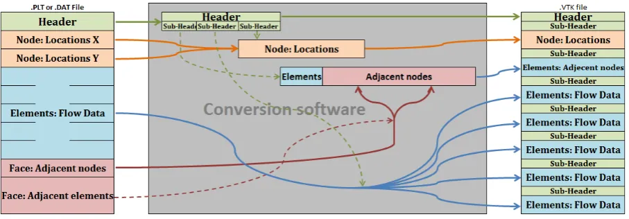
The conversion of the data from the flow solver to a format that ParaView can use was not yet available. Therefore as a part of the assignment, a way to convert this data had to be found. To obtain an easy and quick way to convert this data, a C++ program is written. The code is added to this report in appendix A. In figure 2.1 a schematic overview of the workings of the program is given.

The conversion software converts the data into a VTK file format. This format is chosen for multiple reasons. First of all, it is a file type that can be read by multiple software packages across multiple platforms including ParaView. A second reason is because the files are written in ASCII which means the file is readable as plain text and easier to handle. And last but not least, there were clear guidelines available on the Internet how such files should be built up.

Figure 2.1: Schematic overview of the conversion software

As a first step, the program takes the data file and subtracts all important data from the header. This information contains the names of the variables, and in what order they are stored. The size of each sector is also defined in this section. After this, coordinates of mesh nodes are copied and reordered into an array.

The next step is the most complicated because it converts the face oriented information in cell ori-ented information. In the old file format, for every face two nodes are stored which suspend it, then the elements on each side are listed. In the new file format, the nodes are stored directly with their elements. By storing and sorting the nodes per element, halve of space needed for this data can be saved. In the final step, the data of all cell variables are copied line by line. The converted data can not only be red by ParaView, but also saves up to 25 percent in disc space per output file.

Chapter 3

model validation

Before starting the simulations on the more complex configuration in which cylinder and an airfoil are combined, both situations will be inspected independently. This is done to validate the model and the assumptions that are made for this model. The reference case is based on the parameters that are chosen in the paper ”Unsteady flow simulation around Cylinder under airfoil using Cartesian-based flow solver”6_{, in which the same set-up is studied. Each parameter will be changed one by one, while the} rest of the parameters is kept as in the reference case.

3.1

Single cylinder

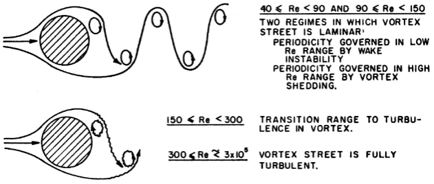
First a single cylinder case will be studied. The single cylinder case is a well studied case for which much is known. An example of this is the shedding regiment and frequency and their dependency on the Reynold number as seen in figure 3.1. This kind of knowledge makes it easier for the parameters to be tested and configured. As an example, important parameters that need to be checked are for example the size of the elements used and the size of the time-steps that are used. The solution should be independent of these parameters while the calculation time should be kept short. In the following paragraphs, each of these parameters will be covered with the single cylinder simulation.

With respect to the cylinder diameter, the Reynolds number will initially be set to 1 000. This is equal to 10 000 with respect to the airfoil. This Reynolds number is actually on the high side, but had to be used because it is the same case in the paper on which the research is based. It can than also be used as a reference case. The reason that the chosen Reynolds number is to high is because turbulence will be present in the vortex street7_{, this will cause the vortexes to break down in three dimensions. This effect} is not taken into account in a two dimensional analysis. The used method is actually more applicable to Reynolds numbers between 90 and 150 in which the flow is assumed to be fully laminar. The accuracy of the two dimensional approximation will be tested. For the first approximation, the expected values for the Strouhal number will be linearly interpolated from the lower Reynold number region.

Figure 3.1: Regimes of fluid flow across circular cylinders7

Figure 3.2: Mesh of the reference case

3.1.1

Mesh size

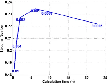
When doing simulations, mesh size is an important part of the considerations that need to be made. The smaller the elements you use, the closer your solution will be to the continuous solution. However the downside of smaller elements is that more elements are needed to cover the same area and thus, more time is needed for all the calculations. The number of elements needed will grow with the order of the dimensions used in the simulation. In a two dimensional case, this means that when the mesh is halve the size,22= 4more elements are needed. This also implies that roughly 4 times more calcula-tion time is needed. Therefore a good balance between mesh size and computacalcula-tional time needs to be sought.

In figure 3.3, the Strouhal number is shown against the calculation time. For rough element sizes , which are on the left side of the image, it is clear to see that a refinement has a positive influence on the estimation of the shedding frequency. For smaller meshes however, this effect diminishes while the time needed for a simulation rapidly grows. In figure 3.4 the power spectrum density in the far field is plotted. This power spectrum density is also calculated by the software delivered by the university of Tokyo. Here, two phenomena are visible. The first one is the shift of the frequencies which is the same effect as seen with the Strouhal number. The Strouhal number is directly connected to the first frequency as this is the frequency of vortex shedding which defines the Strouhal number as shown in equation 3.1. The vortex shedding frequency is defined asf,Lis the characteristic length andU is the speed of the far-field flow.

St= f L

U (3.1)

The shedding from vortexes from the cylinder is slower for a rougher mesh. The second phenomena is the amount of visible frequencies. A rough mesh cannot contain high frequency waves because the wavelength will be to short to be capture in few elements. As a rule of thumb, around 6 elements are needed to describe the acoustic wave. In the case of 0.02*diameter, the acoustic mesh is 0.064. This results in maximum a describable frequency of 2.6 Hz. A mesh that is to fine introduces a lot of noise into the system. The reason for this is not clear.

3.1.2

Field size

The size of the computational domain is of importance because we want a uniform far-field flow. where compressibility and reflection are no issues. Due to build up of the mesh, the cells in the far field are quite large and therefore relatively ’cheap’. Any effects caused by a flow region that is to small should therefore be prevented. In the analysis with a single cylinder, only small influences are noticed. However the far field size should be 100 times the chord size by a rule of thumb.

3.1.3

Other configurations of the mesh

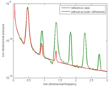
Next to the original mesh configuration, a couple of other configurations are tested. In the first case the refinement box for the acoustic region is left out. The results are as expected. The cells on the outer area are much courser which means that these cells cannot carry the higher frequency waves. It does not change the near field flow however and therefore the forces on the cylinder and the lower frequencies remain the same.

Reference case

Without acoustic refinement Strouhal

number 0.2344 0.2327

Drag

coefficient 1.527 1.516

Lift

coefficient 0.009 0.007

Table 3.1: Parameters without acoustic refinement

Figure 3.5: PSD with and without acoustic mesh

The other alterations on the mesh are considering the wake region. For one case, the wake is not refined. When the wake of the cylinder is not refined, the shedding of the vortexes is not properly sim-ulated. This effect can be seen in the lower Strouhal number and the frequency shift in table 3.2 and figure 3.6.

For the final case, an extra refinement region for the wake is added in which the vortexes move along with the flow. The results from this analysis show that this extra refinement has no positive or negative effect on the frequency peaks and the drag coefficient. However, an artifact at the end of this wake region creates more background noise. Therefore, and for the fact that the computational time is higher, no extra wake region will be implemented.

Reference case Without wake With extra wake Strouhal

number 0.2344 0.2176 0.2341

Drag

coefficient 1.527 1.510 1.526

Lift

coefficient 0.009 -0.005 0.009

Table 3.2: Parameters with changed wake

Figure 3.6: PSD with and with changed wake

3.1.4

Time step

The size of the time steps is import for simulation time dependent data. If the time step is to course, data can be lost. However for simulating the same length of time, the total number of steps needs to increase. The total simulation time is therefore inverse linearly related to the time step. In figure 3.7, the Strouhal number is plotted against the inverse of the time step. Decreasing the step size by half and thus increasing the necessary calculation time by two will only result in a two percent increase in the Strouhal number Therefore, the time-step is chosen to be0.01. The number of iterations needed follows from this number, the amount of time steps it takes to converge to a repetitive signal and the amount of iterations needed for averaging.

Figure 3.7: Strouhal as a function of the time-step size

3.1.5

Number of sub-iterations

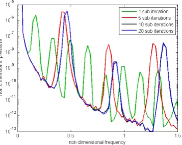
The number of sub-iterations are the number of iterations done before moving on to the next time step. The number of sub-iterations needed is depending on how quick a result converges to the real value. The more sub-iterations are used, the more time it will take per time-step en therefore the more time it will take to finish the simulation. As seen in table 3.3 and figure 3.8 In the case of one and five sub-iterations, the Strouhal number is effected by the small number of sub-iterations. For the case of 10 and 20 sub-iterations, both result in almost the same PSD. Therefore the only 10 sub-iterations will be used.

Number of

Sub-iterations 1 5 10 20

Strouhal

number 0.0879 0.2183 0.2344 0.2342 Drag

coefficient 1.549 1.532 1.527 1.530 Lift

coefficient -0.146 0.062 0.009 -0.005

Table 3.3: Parameters with different sub-iterations

Figure 3.8: PSD with different sub-iterations

3.1.6

Averaging

3.1.7

Reynolds Number

As mentioned at the beginning of this chapter, the flow regiment for which this situation is valid has a Reynolds number between 90 and 150. The results above are all obtained at a Reynolds number of 1000. Therefore only the amount of change due to refinement in the Strouhal number, drag and lift coefficients are checked and not if they converge to the expected value. In this last paragraph, the case with the found parameters is used for different Reynolds numbers. For the cases with a smaller Reynolds number, the values can be checked if they are close to known values.

Reynolds

number 100 150 300 600 1000

Strouhal

number 0.1648 0.1844 0.2105 0.2275 0.2344 Drag

coefficient 1.353 1.345 1.397 1.458 1.527 Lift

coefficient-0.001 0.001 0.000 0.000 0.009

Table 3.4: Parameters different Reynolds numbers

Figure 3.9: Strouhal to Reynolds number

3.2

Airfoil

In this chapter the single airfoil case is studied. This done with two reasons. First of all, a simplification is done on the boundary in which a slip boundary condition is implied. It should be tested if there is a difference between the Navier-Stokes calculations, which are done for this simulation, and the Euler equations which are used for inviscid flows. Due to the non viscosity, these equations normally need the non slip boundary condition. The second reason is to verify the findings with the paper Unsteady flow simulation around cylinder under airfoil using Cartesian-based flow solverCartesianFlowSolve. In this paper the same software is used to look at a similar situation. Therefore the results should also approximately be the same.

3.2.1

Boundary condition

As said before, the boundary condition that is applied to the airfoil is a slip boundary condition. It is verified if the Navier-Stokes and the Euler equations give approximately the same results. The difference in these methods doesn’t lie in the fact that the normally applied boundary condition is different, but comes from the fact that the Euler equations govern the inviscid flows while Navier-Stokes takes this viscosity into account. Therefore at a slip boundary on a thin object in a flow, the influence of the calculation method should be small. In the figures 3.10 and 3.11, the flow speed in X-direction is shown for the Navier-Stokes and Euler cases respectively. Incoming flow has angle of 4 degrees. The

Figure 3.10: Flow speed over the top boundary with Navier-Stokes

difference is visible in these plots but the effect is very small. Plots are made to get a closer look at the flow variables near the edge. In figure 3.12 the regions over which is plotted are shown. The result in figures 3.13 and 3.14 show that there are only minor differences between the two calculation methods.

Figure 3.12: Regions over which the flow values are plotted

Figure 3.13: Flow values at the front side of the air-foil

Figure 3.14: Flow values at the rear side of the air-foil

3.2.2

Angle of attack

In this section, the same cases as in the paper Unsteady flow simulation around cylinder under airfoil using Cartesian-based flow solver are solved. This is done for the cases with alpha 0 and 4. As shown in table 3.5, the cases for the single airfoil are approximately the same.

Drag Lift

Angle 0 Angle 4 Angle 0 Angle 4

Reference Paper 0.009 0.018 0.000 0.476

Current simulations 0.008 0.016 0.000 0.471

Chapter 4

Interaction between Cylinder and

Airfoil

In this chapter, the interaction between the cylinder and the airfoil will be studied. It is assumed that the cylinder partially obstructs the flow, thus slowing it down at the lower side of the airfoil. It is assumed that this will influence the lift coefficient of the airfoil. The influence of the airfoil on the cylinder is also assumed to be mainly a flow speed difference. The flow speed is shown to be of a large influence on the acoustic power of the shedding noise8. furthermore, this change in flow speed could possibly influence the shedding frequency of the cylinder and thereby change the frequency of tonal sound measured. At last but not least, the airfoil acts as a barrier which might deflect the noise, coming from the cylinder back downward. In the next section, these assumptions will be verified. Furthermore, alterations to the set up will be made to investigate the influence of these changes.

4.1

influence of Cylinder on Airfoil

As mentioned in the introduction of this chapter, it is assumed that the presence of the cylinder will cause the flow at the bottom side of airfoil to slow down. This on its turn, increasing the pressure on the bottom side of the airfoil and thereby causes an increase in lift. This assumption appears to be true for a small angle of attack and is visible in the images 4.1 and 4.2. The lift coefficient is increased from 0 to 0.089. For a little larger angles of attack the increase in lift due to the presence of the cylinder

Figure 4.1: Mach number on the airfoil surface

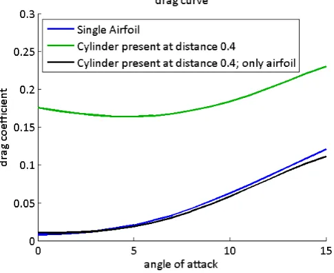
is slightly decreasing. At even larger angle of attacks (larger than 12 degrees) the lift of the airfoil decreases due to the presence of the cylinder. The point of most lift decreases both in hight and angle of attack due to cylinder presence. For high angles of attack, the drag of the airfoil is reduced by the presence of the cylinder. This is due to the fact that for higher angles of attack, the airfoil moves toward the wake of the cylinder.

For smaller angles attack, the drag on the airfoil also increases, while for larger angles of attack the drag on the airfoil decreases, as can be seen from image 4.3. From this fact, and from what we seen in the lift curve, we could conclude that for small angles of attack, the local angle of attack on the airfoil is increased. For larger angles of attack, the airfoil will have less drag and lift from the flow, because the airfoil will move into the wake of the cylinder. Next to the change in the airfoil flow, the cylinder introduces a lot of drag of its own to the system. Introducing a cylinder would therefore not improve flight conditions of an airfoil.

Figure 4.3: change to drag-curve (total and airfoil only) with presence of the cylinder

An important thing to mention is the following. Under the conditions at which the airframe is spectacled, a steady solution gives the same result as a transient solution because the flow around the airfoil is steady. When the cylinder is introduced, the flow field around the airfoil changes. The airfoil will not only be subjected to another flow field, but the flow field will also be transient and therefore cannot be analyzed with the steady analysis. From the result in figure 4.4 we can see that the assumtion U(t)=U(0)+U’ does not imply that a steady solution could be used because U’ does have influence on the drag and lift coefficient. It should be kept in mind that even though the assumptions made for an easy case apply well, the situation might change when other factors are applied like an extra geometry.

4.2

Influence of Airfoil on Cylinder

It was assumed that the influence of the airfoil on the cylinder is both aerodynamically and acoustic. The presence of the airfoil will probably influence the flow field which lead to different drag and lift coefficients as well as a different shedding frequency. For low angles of attack the drag on the cylinder increases, the flow speed on the side of the airfoil increases. Therefore the drag on the cylinder will be larger. For larger angle of attacks. The stagnation region of the airfoil will move to the bottom side of the airfoil. The cylinder will therefore have to coop with a smaller flow speed which will cause the drag on the cylinder to decrease. Because the flow along the airfoil is deflected a little, the local incoming flow on the cylinder will be directed downward a little. This causes a negative lift coefficient in global coordinates.

Figure 4.5: Strouhal Number in the presence of an airfoil

The Strouhal number is also a little bit higher at low angles of attack and lower at higher angles of attack. This is also caused by the fact that the incoming flow is disturbed by the airfoil. The Strouhal number is scaled with the flow speed of the far field. However, due to airfoil the local speed is a little increased for small angles of attack and decreased for large angles of attack. This will cause other shedding frequencies.

Figure 4.6: Acoustic effects due to the airfoil

4.3

location of the cylinder

In the paper ”Unsteady flow simulation around Cylinder under airfoil using Cartesian-based flow solver”6 it was shown that the location on of the cylinder was important for the strength of the effect with which the two geometries influence each others flow-field. This is logical because a flow is more disturbed closer to an object, and therefore the disturbance felt by the other geometry is also larger when it is closer to the object. In the paper ”Unsteady flow simulation around Cylinder under airfoil using Cartesian-based flow solver” only two points are compared at different distances from the center of the airfoil. In this chapter, more values for the distance are checked. After that the influence of the cylinder location along the length of the airfoil is checked and finally a grid of locations is made to see the differences in the influence in the full area. After this, the size ratio between the airfoil and the cylinder will also be inspected.

4.3.1

distance to the airfoil

When the cylinder gets closer to the airfoil, the effects due to its presence increase. This means that for low angles of attack, the lift increases while for higher angles of attack, the lift decreases. The drag also increases a little bit further. When getting to close to the airfoil however, these effects tend to get out of hand and are non realistic.

Figure 4.7: Effects of distance between airfoil and cylinder

In figure 4.7 it is visible that for distances larger than 0.3c the effects on the drag and lift are almost linearly increasing. If the distance gets smaller the effects are not linear and predictable anymore. In figure 4.8 we can see that for distances smaller than 0.3 the lift curve makes a jump in lower angles of attack while for high angles of attack the results return to normal. It can be concluded that for low angles of attack and small gap sizes, a strange anomaly occurs. For both higher angles of attack and larger gap sizes this does not occur and the results look normal. These effects will be explained in the paragraph ’small gap artifacts’ (paragraph 4.3.4).

4.3.2

location in flow direction

When the cylinder is placed at different locations along the length of the airfoil, different lift and drag coefficients are found. The location in this direction is therefore also inportant. As can be seen in image 4.9. The drag is highest when the cylinder is placed in the middle of the airfoil and is smaller when the cylinder is placed towards one of the edges of the airfoil. For larger angles of attack, the placement of the cylinder where the maximum drag occurs shifts backward. The least drag will then occur when the cylinder is placed near the leading edge. For the lift, a maximum is found near the trailing edge. For larger angles of attack this effects are still there, although the effect will be small compared to the effect induced by the angle of attack.

Figure 4.9: Lift and Drag coefficients at distance 0.4

In the downward direction, the acoustic power caused by the flow around the cylinder is largest when the cylinder is placed at 0.3 chord length from the leading edge. This is possible due to the fact that more sound is reflected by the airfoil, and the direction in which the sound is reflected is downward as well. The effects however are relatively small and therefore hard to see in in figure 4.10. When the cylinder is near one of the edges, more waves can go upward and the reflection by the airfoil is more horizontally oriented. At a low angle of attack, the frequency of the sound is higher when the cylinder is near the trailing edge. When the angle of attack increases, the lower frequency is on both edges. On the upper side of the airfoil, a region with low sound levels is present. This might be caused by the fact that the airfoil is directly in the way of the sound waves. Those sound waves that are then traveling around both edges arrive in opposing phase at the measuring point, causing destructive interference.

Figure 4.11: Polar plot at first frequency due to streamwise cylinder location

4.3.3

location of the cylinder in 2-D

When varying both the distance to the airfoil and the stream-wise location of the cylinder, a grid can be created to show a landscape diagram of the lift and drag on the combined geometry. Far away from the airfoil, this landscapes looks like a neat curved plane. When getting closer to the airfoil however, the landscapes starts to become rough and inconsistent, some of the effects occurring also seem the be counter intuitive. In image 4.12 for example, the lift coefficient drastically increases for a distance of 0.2c under the thicker part of the airfoil. For distances over 0.3c the results look more like a surface. This also looks to be the case for smaller distances when the cylinder gets closer to the trailing edge.

Figure 4.12: Surface plot of Lift coefficient for multiple cylinder locations

In figure 4.13, we can see that in the same locations, and thus in the same simulations, the drag coefficient of the total geometry drops. The effects that are mentioned will be further analyzed in the paragraph ”small gap artifacts”. If we ignore these result for now, the conclusion would be that the best lift and drag coefficients are found if the cylinder is placed near the edges of the airfoil, and mainly the trailing edge in small proximity to the airfoil.

Figure 4.13: Surface plot of Drag coefficient for multiple cylinder locations

of other analysis. The drag differs largely from place to place and increases a lot and the lift increases substantial. Next to these huge changes in the forces on the geometry, a lot of broad spectrum noise is measured and visible in the PSD plots. To see why the forces on the geometry differ so much, the time dependent forces are inspected relative to an estimated average. The estimated average is based on figure 4.8 in which the low lift coefficients are assumed to be linear depending on the angle of attack. In figure 4.14 the deviation of the lift in four cases are shown. The first two cases are either with a large gap size, or a large angle of attack. These cases have a structured wave around their average value. For an angle of 0 degrees, the lift deviation does not look as wave like as the other two simulations do further more, the whole signal lies above the estimated average. For an angle of attack of 3 degrees, the signal first appears to be stable around the estimated average before the lift also increases. As a side note it could be mentioned that, although the two latter cases are compared with estimated values, the start up effects look similar to the stable cases. This is not the case if the average lift is used that is plotted in 4.8. This implies that at the start, the solution tries to converge to the estimated value before it destabilizes.

Figure 4.14: deviation of lift coefficient

the top and bottom cases, alternating vortexes are created which then start to form two shear layers. In the middle case, which is the case for a small gap and a small angle of attack, the vortexes shed and fall apart in a more chaotic way.

Figure 4.15: Vorticity at time step 12000 for three different cases

The time averaged Mach number around the geometry is plotted in figure 4.16. From left to right, these are again the cases for a distance 0.4 chord lengths and angle 0 degrees, a distance 0.2 chord lengths and angle 0 degrees and a distance 0.2 chord lengths and angle 9 degrees. The middle case does again differ from the other two in a way that under the airfoil trailing edge, a stagnation region exists in which the flow speed drops close to 0 Mach. There could not be found any explanation for this phenomena. From the papers about a flow around a cylinder near a plane9,10, it could be said that an coupling between the boundary layer on the airfoil and the shedding of the cylinder exists. The ratio of the gap size over cylinder size would then be of influence for the shedding regiment. The effects mentioned in these papers do however involve the boundary layer on the plane, which is absent on to airfoil for the implied boundary conditions.

Figure 4.16: Time averaged Mach number

To see if the boundary on the airfoil is of influence on this effect the boundary condition is changed to a non-slip boundary. The mesh size on the wall is also changed to the 0.001c from 0.004c.

4.4

cylinder size

As part of the research, the size of the cylinder is changed at a distance of 0.4 cord lengths from the midpoint of the airfoil. The range of diameters that is tested lies between 0.05c and 0.15c with a change in the diameter 0.01c per simulation. In this paragraph, the results for the larger cylinder sizes are shown in red and the smaller cylinder sizes are depicted in blue. The variations in the geometry are shown in image 4.17.

Figure 4.17: Overview of the geometry for different cylinder sizes

on the drag of the airfoil, or at least not at this distance.

Figure 4.18: Drag coefficient of cylinder and the whole geometry for different cylinder sizes

Figure 4.19: Strouhal Number for different cylinder sizes

Figure 4.20: First peak for the Power Spectrum Density measured in downward direction

Chapter 5

conclusion

The goal of this report was to create more insight in the interaction between the landing gear and a wing. This case is greatly simplified for the sake of computation time and simplicity of the problem. The study is done in a two dimensions, the landing gear is replaced by a circle to represent a wheel and the wing is replaced by a symmetrical airfoil. For this simplified case, the validation was derived from known simple cases like the separate cases of the cylinder and the airfoil. From these simulations a set up could be derived witch could correctly calculate the solution for this problem. The 2D assumption for a Reynolds number of 10 000 is not fully correct and the result might therefore differ from a real live scenario. This is due to the fact that in natural conditions three dimensional turbulence would occur. This implies that the actual shedding frequency is lower than the one shown in the simulations.

First a lift curve was constructed for the airfoil an for the case where the cylinder was placed at a distance of 0.4 chord-lengths from the airfoil center. A small increase for the lift was noticed on small angles of attack, a drop in lift was noticed for larger angles of attack. The case where the cylinder was placed at a distance of 0.2 chord lengths for the airfoil center showed a larger increase in lift was visible for small angles of attack and a bigger decrease for high angles of attack. When the angle of attack was to low however, a jump and irregularity in the lift was found for this case. These solutions seem to be incorrect. The same effect was visible for other locations of the cylinder where the distance between cylinder and airfoil was small.

For the location of the cylinder minor changes can be seen in the lift and drag coefficients. The change in acoustic spectrum is better visible because small changes in the flow speed will have a more noticeable influence on the frequency and magnitude of the sound that is generated. Next to that, the sound profile is influenced by airfoil by blocking and reflecting the sound waves. The relative location of the airfoil to the cylinder is therefore of importance.

References

[1] R. G. Psuhkar, “Comet’s tale,”Smithsonian Magazine, 2002 June 2002. [2] D. P. Lockard, “The airframe noise reduction challenge,”

[3] W. Dobrzynski, “Almost 40 years of airframe noise research: What did we achieve,” [4] S. M.J.T.,Aircraft Noise.

[5] Y. P. Guo, “Experimental study on aircraft landing gear noise,”

[6] T. Imamura and Y. Takahashi, “Unsteady flow simulation around cylinder under airfoil using cartesian-based flow solver,”

[7] J. H. Lienhard, “Synopsis of lift, drag and vortex frequency data for rigid circular cylinders,” 1966. [8] T. N. Krasil’nikova, “Dipole nature of sound radiation by free turbulance,”

1 C:\Users\Mark\Desktop\Internship\...\VtkConverterSingleFile\VtkConverterSingleFile.cpp

/*File te translate flow-data files to vtk format (Legacy format) Made by Mark Böke*/

#include <iostream> #include <fstream> #include <string> #include <vector> #include <sstream>

using namespace std;

int main() {

string filename; string newfilename;

//open a file of the users choise; will normaly be .plt or .dat format

cout<<"Please input the name and extension of the file you wish to convert \n"; cout<<"if the file is not in the same folder, type whole adress \n";

cin>>filename; cout<<"\n";

size_t length=filename.find_last_of("."); //find the extension

newfilename=filename.substr(0,length); //remove extension from the name newfilename.append(".vtk"); //add new extension

cout << "\nNew file will be called: " << newfilename << "\n \n";

ifstream oldfile (filename); //open the choosen file if (oldfile.is_open())

{

//Global variables

int nNodes (0); //number of nodes

int nFaces (0); //number of faces

int nElements (0); //number of elements

int nVariables (0); //number of variables

int nData (4); //number of data that needs to be required before

moving on

std::vector<string> variableNames; //list of names of variables

std::string fileLine; //string used

int posNodeData (0); //position of the first nodal data (X,Y) used for

intiation of data copying

int posElementData (1); //position of the first elemental data (Rho, U, V,

P, Cp, Mach, aux) used for intiation of data copying

int nCellPoints (0); //counts the total number of nodes in all cells

together; most nodes therefore are multiple times counted; used in vtk datatype

//Read Overall data (Number of Nodes,Elements,Faces,Variables and Names of Variables)

while (oldfile.good()) //this means if no flag occurs

{

std::string searchQueryN ("Nodes="); //search querry used to find the data about the number of nodes, this is case sensitive

std::string searchQueryF ("Faces="); //search querry used to find the data about the number of faces, this is case sensitive

std::string searchQueryE ("Elements="); //search querry used to find the data about the number of elements, this is case sensitive

std::string searchQueryV ("VARIABLES="); //search querry used to find the data about the amount and names of the variables, this is case sensitive

std::size_t strtSelect; //local help parameter for cutting text std::size_t endSelect; //local help parameter for cutting text getline(oldfile,fileLine);

strtSelect=fileLine.find(searchQueryN); //searches for "Nodes="

if (strtSelect!=std::string::npos) //if the search statement did not return the end of line position

{

strtSelect+=searchQueryN.length(); //puts the begin marker

after the searchquerry

endSelect=fileLine.find(",",strtSelect); //finds the delimiter and puts the end marker there

string alfa=fileLine.substr(strtSelect,endSelect-strtSelect); //copy's the number from the file as text

2 C:\Users\Mark\Desktop\Internship\...\VtkConverterSingleFile\VtkConverterSingleFile.cpp

into an integer

nData--; //one less datatype to

find }

strtSelect=fileLine.find(searchQueryF); //searches for "Faces="

if (strtSelect!=std::string::npos) //if the search statement did not return the end of line position

{

strtSelect+=searchQueryF.length(); //puts the begin marker

after the searchquerry

endSelect=fileLine.find(",",strtSelect); //finds the delimiter and puts the end marker there

string alfa=fileLine.substr(strtSelect,endSelect-strtSelect); //copy's the number from the file as text

nFaces=atoi(alfa.c_str()); //conversion of the text

into an integer

nData--; //one less datatype to

find }

strtSelect=fileLine.find(searchQueryE); //searches for "Elements="

if (strtSelect!=std::string::npos) //if the search statement did not return the end of line position

{

strtSelect+=searchQueryE.length(); //puts the begin marker

after the searchquerry

endSelect=fileLine.find(",",strtSelect); //finds the delimiter and puts the end marker there

string alfa=fileLine.substr(strtSelect,endSelect-strtSelect); //copy's the number from the file as text

nElements=atoi(alfa.c_str()); //conversion of the text

into an integer

nData--; //one less datatype to

find }

strtSelect=fileLine.find(searchQueryV); //searches for "Variables="

if (strtSelect!=std::string::npos) //if the search statement did not return the end of line position

{

endSelect=strtSelect; //puts

endSelect at the start of the Variables area for the following alternating search querry

while(endSelect<fileLine.length()&&strtSelect<fileLine.length()) //as long as the two markers are within the length of the line

{

strtSelect=fileLine.find("\"",endSelect+1)+1; //find

the first next "-sign and put the begin marker here

endSelect=fileLine.find("\"",strtSelect+1); //

finds the first next "-sign and put the end marker here

if(endSelect>0&&strtSelect>0) //only

perform this action if the line did not accidentaly started over

variableNames.push_back(fileLine.substr(strtSelect,endSelect-strtSelect)); //copy 's variable name from the file

else break; }

nVariables=variableNames.size(); //

count the number of variables extracted

nData--; //one

less datatype to find }

if (nData<=0) //if all datatypes are found, stop searching

break; }

std::cout << "Overall Data found\n";

//Finds first numerical line

oldfile.seekg(0); //go to begin of the file

while (oldfile.good()) //this means if no flag occurs

3 C:\Users\Mark\Desktop\Internship\...\VtkConverterSingleFile\VtkConverterSingleFile.cpp

zero every line

posNodeData=oldfile.tellg(); //safe the beginning of this line

as the first nodal data

getline(oldfile,fileLine); //read a new line from the file

found=fileLine.find_first_not_of(" -.0123456789",1); //starting from position one, if this line does contain another symbol, found gets that position

if (found==0||found>fileLine.length()) //if found is eather zero or to large, the line does not contain another symbol

break; }

std::cout << "position of first numerical data is: " << posNodeData << "\n"; /* Gathering of global data is finished */

//Create fresh flowCart.vtk file

ofstream newfile (newfilename); //creates an empy vtk file with the same name as the original file

if (newfile.is_open()) //if this works

{

newfile << "# vtk DataFile Version 3.1\n"; //These four lines are basic information for opening the vtk file

newfile << "This Flow data is converted to vtk format\n"; //which will be at the head of the file

newfile << "ASCII\n"; //

newfile << "DATASET UNSTRUCTURED_GRID\n"; //

//Copy Nodal location data (X and Y)

newfile << "POINTS " << nNodes << " FLOAT\n"; //The basic information for the points is written in the file

vector<vector<float>> nodeLocation(nNodes, vector<float>(3)); //A new vector is created in which the data of all nodes will be temporarily stored

oldfile.seekg(posNodeData); //Reset the reading point of

the plt file to the beginning of the nodal data

for (int i=1; i<=nNodes; i++) //copy all X data //Repeat the next part once for every node:

{

getline(oldfile,fileLine); //extract a line from the plt

file

nodeLocation[i-1][0]=atof(fileLine.c_str()); //convert it to a number and then store it in the vector (as x-data)

}

for (int i=1; i<=nNodes; i++) //copy all Y data //Repeat the next part once for every node:

{

getline(oldfile,fileLine); //extract a line from the plt

file

nodeLocation[i-1][1]=atof(fileLine.c_str()); //convert it to a number and then store it in the vector (as y-data)

nodeLocation[i-1][2]=0; //set z data to 0 //store a 0 in vector (as z-data) because the result is 2D and thus has no z component

}

for (int i=1; i<=nNodes; i++) //for every node: save the

data in the vector to the vtk file

newfile << 1][0] << "\t" << 1][1] << "\t" << nodeLocation[i-1][2] << "\n";

std::cout << nNodes << " lines of nodal data converted \n";

posElementData=oldfile.tellg(); //ask location to later find

the location of the data for the variables

nodeLocation.~vector(); //destroy the vector with

temporary data for the vectors

//First skip all Variables Data

for (int i=1; i<=nElements*(nVariables-2); i++) //for all non X and non Y variables

{

getline(oldfile,fileLine); //skip this line (nothing is

done with fileLine) }

std::cout << "Variables data skipped \n";

//Create Element location data (suspension nodes)

4 C:\Users\Mark\Desktop\Internship\...\VtkConverterSingleFile\VtkConverterSingleFile.cpp

vector<vector<int>> elementData(nElements, vector<int>(17)); //create a vector for the element data which will be reconstructed from the face data; 17 rows for a maximum of eight faces (of two data points) and one counting value

for (int i=1; i<=nFaces ; i++) //repeat the next section for

every face {

getline(oldfile,fileLine); //get information form the plt

file

std::stringstream stream(fileLine); //make a stream of this line

stream >> faceData[i-1][0]; //get the number of the first

node from the steam

stream >> faceData[i-1][1]; //get the number of the second

node from the stream }

std::cout << "Nodal data of faces aquired \n";

for (int i=1; i<=2*nFaces ; i++)//link nodal data to elements //for every face this has to be done two times

{

getline(oldfile,fileLine); //read which element contains

this face

int elementNumber=atoi(fileLine.c_str())-1; //convert this element number to an integer

if (elementNumber>=0) //if the element number

excists, do the following {

int n; //

create a temporary counter

if (i<=nFaces) //if i

is smaller then the number of faces, i needs to be used hereafter

n=i; //

else //if i

is larger then the number of faces, we should start counting again (or substract the number of faces)

n=i-nFaces; //

elementData[elementNumber][elementData[elementNumber][0]+1]=faceData[n-1][0]; // store the first nodal data for this face in the first free spot in the element data vector

elementData[elementNumber][elementData[elementNumber][0]+2]=faceData[n-1][1]; // store the second nodal data for this face in the second free spot in the element data vector

elementData[elementNumber][0]+=2; //put

the information of two extra filled cells in the counter cell }

}

std::cout << "Elemental data of faces aquired \n";

//the element data will now look as follows [8 nodes (1 2) (3 4) (3 2) (4 1) 0 0 0 0 0 0 0 0]

for (int i=0; i<nElements; i++) //cleaning up nodal data of the elements //do the following for every element

{

for (int j=2; j<elementData[i][0]; j++) //start at the

second node and do this for every node: {

int k=j+1; //for all cells

behind the current one while (k<16) {

if (elementData[i][j]==elementData[i][k]) //search for

another cell with the same information {

if (k % 2) //if this double

information is in an odd cell {

std::swap(elementData[i][j+1],elementData[i][k]); //switch the location of the same information with the cell behind the first one

std::swap(elementData[i][j+2],elementData[i][k+1]); //switch the other node (from the same face) with the cell therafter

}

else //if this double

information is in an even cell {

5 C:\Users\Mark\Desktop\Internship\...\VtkConverterSingleFile\VtkConverterSingleFile.cpp

location of the same information with the cell therafter

std::swap(elementData[i][j+1],elementData[i][j+2]); //switch the two nodes of the face in position

}

} //after this, the element data looks as follows [8 nodes (1 2) (2 3) (3 4) (4 1) 0 0 0 0 0 0 0 0]

k++; }

}

elementData[i][0]=elementData[i][0]/2; //now the number

of nodes is halved (because every node is displayed double)

for (int j=1; j<=elementData[i][0]; j++) //for all nodes

elementData[i][j]=elementData[i][j*2-1]-1; //copy their

number and put them in the spot where they will end up in; also substract 1 because vtk starts its nodal information with node 0

for (int j=elementData[i][0]+1; j<17; j++) //for all non

nodes

elementData[i][j]=0; //these will be

zero

nCellPoints+=elementData[i][0]+1; //count the number

of nodes in this cell and also count the information cell (for the way vtk reads is data herafter) }

std::cout << "Elemental data completed \n";

newfile << "\nCELLS " << nElements << " " << nCellPoints << "\n"; //save the basic line for the elements in the vtk file

for (int i=0; i<nElements; i++) //for every

element {

newfile << elementData[i][0] << "\t"; //save the number of nodes for this element

for (int j=1; j<=elementData[i][0];j++) //for every node

in this element {

newfile << elementData[i][j] << "\t"; //save the number of this node in the same line

}

newfile << "\n"; //start a new line

for the next node }

newfile << "\nCELL_TYPES " << nElements << "\n"; //save the basic line for the element type in the vtk file

for (int i=1; i<=nElements; i++) //for every

element

newfile << "7 "; //save element

type 7 (polygon)

newfile << "\n";

std::cout << nElements << " lines of element data converted \n";

//Copy Element Variables data

oldfile.seekg(posElementData); //go back to the

point where all the data of the variables was stored

newfile << "\nCELL_DATA " << nElements << "\n"; //save the basic line for all variable data for element centered data

for (int i=2; i<nVariables; i++) //for all the

variables individualy {

newfile << "SCALARS Cell_" << variableNames[i] << " FLOAT\n"; //save the basic lines for this variable

newfile << "LOOKUP_TABLE default\n"; //

for (int j=1; j<=nElements; j++) //for every

element {

getline(oldfile,fileLine); //load a line from

plt file

newfile << fileLine << "\n"; //save it to the vtk file

}

newfile << "\n"; }

6 C:\Users\Mark\Desktop\Internship\...\VtkConverterSingleFile\VtkConverterSingleFile.cpp

std::cout << "succesfully created vtk file \n"; //if everything went well, the following line should print and the file will close

} else {

cout << "Unable to create file\n"; //the following

error occurs if there could not be made a new file named flowcart.vtk system("pause");

}

oldfile.close(); }

else {

cout << "Unable to open file\n"; //the following

error occurs if there couldn't be a file opened named flowCart.plt system("pause");

}