Design of a Matlab based graphical user interface for visualization and enhancement of floor dynamics

(1)

Internship report: Design of a Matlab

based graphical user interface for

visualization and enhancement of floor

dynamics

F.B.Koopman

s0166626

Document name: Report_fkoo.docx

Date: 23 July 2018

MECAL, Enschede, The Netherlands

Supervisor Mecal: Servaas Bank

Internship period: 1/5/2018-31/7/2018

University of Twente

Faculty of Engineering Technology

(2)

Form ID: HTS-QF-014-v3 Form Issued: January 2017

Report_fkoo.docx ©MECAL 2018 Confidential

Page 2 of 151

Internship report: Design of a Matlab based graphical

user interface for visualization and enhancement of

floor dynamics

Document name:

_{Report_fkoo.docx}

Date:

23/07/18

Written by:

Frederik Koopman, MECAL, Enschede, The Netherlands

Reviewed by:

Servaas Bank, MECAL, Enschede, The Netherlands

Approved by:

Servaas Bank, MECAL, Enschede, The Netherlands

Document by:

_{MECAL, Enschede, The Netherlands}

Mailing list:

_{MECAL (1x)}

Pages incl. cover:

₁₅₁

Keywords:

_{Floor vibrations, floor vibrations reduction, floor dynamics}

Language:

_English

Software version:

_{Microsoft Word 2016}

Contributing Authors

Name Author

Part(s) of this document

Frederik Koopman

All

Document change and history record

Version

Date

Page (s)

Short description

1.0 23/07/18

151 First Issue

(3)

Page 3 of 151

Summary

(4)

Page 4 of 151

Summary ... 3

Preface and acknowledgements ... 6

Chapter 1 Introduction ... 7

1.1 Assignment description ... 7

1.2 Outline of the report ... 7

Chapter 2 Floor insight GUI ... 8

2.1 Existing version: 1D ... 8

2.2 First new version: 2D ... 9

2.3 Second new version: 2D with floor parameters ... 11

2.4 Third new version: 3D with floor parameters ... 11

2.5 Fourth new version: 3D with floor parameters and not square floors ... 12

Chapter 3 Floor model estimation ... 14

3.1 Higher DOF systems ... 14

3.2 Matrices estimation ... 15

Chapter 4 Matlab based GUI ... 17

4.1 Loading of data ... 17

4.2 GUI functions ... 19

4.2.1 Plotting frf for z, v and/or a with coherence ... 19

4.2.2 Run ODS ... 19

4.2.3 Adding a point mass, frames or point stiffness ... 19

4.2.4 Add of EQs ... 19

4.2.5 Plot sensitivity ... 20

4.2.6 Plot vibrations ... 20

4.2.7 Plot EQ forces ... 20

4.2.8 Save session ... 21

4.3 Code ... 21

Chapter 5 Test case ... 22

Chapter 6 Conclusions and recommendations ... 25

6.1.1 Conclusions ... 25

6.1.2 Recommendations... 25

6.1.3 Experiment ... 25

6.1.4 Retuning of tunable EQs ... 25

(5)

Page 5 of 151

6.1.6 Loading of vibration levels specification ... 26

6.1.7 Adding of point damper and damper parameter to frame ... 26

References ... 27

Appendix A MECAL ... 28

Appendix B Reflection... 29

Appendix C Matlab floor insight GUI code 2D Version ... 30

Appendix D Matlab floor insight GUI code 2D Version with floor parameters ... 38

Appendix E Matlab floor insight GUI code 3D Version with floor parameters ... 46

Appendix F Function globalMatrixBuilder code ... 55

Appendix G Matlab floor insight GUI code 3D Version with floor parameters and variable floor size57

Appendix H Equations.pdf ... 67

Appendix I High to low order estimation Matlab code ... 68

Appendix J Matrices estimation Matlab code ... 71

Appendix K GUI code ... 74

Appendix L Test case table Matrices estimation Matlab script ... 149

Figure 1: 1D floor GUI ... 8

Figure 2: 1D floor system ... 8

Figure 3: 2D floor system ... 9

Figure 4: 2D floor GUI ... 10

Figure 5: floor support assumption ... 10

Figure 6: 2D floor GUI with floor parameters ... 11

Figure 7: 3D floor GUI ... 12

Figure 8: 3D floor GUI for not square floors ... 13

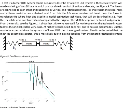
Figure 9: Dual beam element system ... 14

Figure 10: high to low DOF system ... 14

Figure 11: Measurement points example ... 18

Figure 12: Closed-loop system, altered from [6] ... 20

Figure 13: Test case table with SpecTest hammer and sensors ... 22

Figure 14: Table grid ... 23

Figure 15: Table Co-located transfers ... 23

Figure 16: MECAL organogram ... 28

(6)

Page 6 of 151

Preface and acknowledgements

This report is drafted for MECAL and University of Twente, as a conclusion of my 3 months internship

at MECAL from May 1, 2018 until July 31, 2018. During the final year of the master Mechanical

Engineering (Mechanics of Solids, Surfaces and Systems) at the University of Twente, an internship at

an external party must be done. The goal of this internship is to acquiring work experience outside

University of Twente of a trainee or recently graduated engineer level with the main objective of

putting acquired knowledge and skills into practice while the experiences of applying and writing

reports as well as working in expert teams play an important role too.

I chose to do my internship at MECAL since my internship options abroad were cancelled and I needed

an internship fast, this was possible at MECAL. Nevertheless I had a great time during my internship.

While my master was focused mainly on mechatronics this internship was mostly dynamics.

Information on MECAL can be found in Appendix A.

Acknowledgments

The opportunity for doing my internship at MECAL was a great chance for learning and professional

development. Therefore, I consider myself as a very lucky individual as I was provided with an

opportunity to be a part of it. I am also grateful for having a chance to meet so many wonderful people

and professionals who led me though this internship period.

(7)

Page 7 of 151

Chapter 1 Introduction

Mecal High-tech/Systems solves vibration problems for the semiconductor fabrication industry. Mostly the

vibration problems are solved with machine support frames or pedestals, structural building improvements

or by use of EQUALIZER(s) [1] (EQ). The EQ is an active inertial damper system. A big disadvantage of this

method is that it is very time consuming [2].

To get the best results with the EQ the floor needs to be modeled. At the moment this is done based on fitted

FEM calculations, or the EQ are placed using common sense. Previous interns have tried to using the modal

description [3] to get an model for the floor. This method works by getting the mode shapes at the

corresponding eigenfrequencies. The more eigenmodes are known the more accurate the model becomes.

A big advantage of this method is that not all transfer needs to be known just all transfer from all inputs to a

single output. The eigenfrequencies are found by looking for peaks in the absolute value of the transfer or

points were the phase of the transfer passes the points -90 or 90 degrees with a negative slope. The

corresponding mode shapes are gotten by taking the imaginary part of the transfer at these frequency. This

method is known under the name quadrature picking.

While this method works well in theory, in practice there are a few issues. Firstly with systems that have a

lot of damping or having eigenfrequencies that are close together the eigenfrequencies are not easily

identified which can lead to missing eigenmodes. Also the transfers need to have enough eigenfrequencies

to get enough eigenmodes, so measurements needs to have high frequency data.

1.1 Assignment description

At the starting of this internship the assignment was only a global descripting because it was yet unsure

which direction this internship will take. The general idea was to get an even better understanding of

vibrations in floors, how to model it and to be able to measure these vibrations and process the results more

efficiently. This last step is still done with custom Matlab scripts, FEM calculations and simple tests for each

case.

1.2 Outline of the report

(8)

Page 8 of 151

Chapter 2 Floor insight GUI

2.1 Existing version: 1D

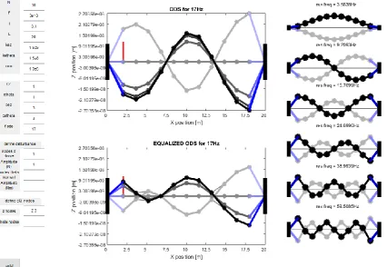
[image:8.595.74.465.302.570.2]

The original floor GUI, see Figure 1, made by Servaas Bank is an insight tool for vibrations in a floor. This GUI

approximates the floor as a series of masses connected by springs that only move in the vertical direction,

see Figure 2. The floor is assumed to be homogeneous in mass and stiffness. The floor is connected to the

fixed world by support springs. The tool asks the user for the number of masses it should use, the stiffness

in the middle of the floor the support spring stiffness, the total mass of the floor and the damping coefficient

for both the floor and support.

Figure 1: 1D floor GUI

The tool calculates the first six eigenmodes of the system and displays them on the right. Also the user can

give 1 or more harmonic forces on the masses and the response is calculated and displayed in the middle top

figure. The user can also give the locations of EQs and the response with the EQs is calculated in the middle

bottom figure.

(9)

Page 9 of 151

The tool works by making a global stiffness, damping and mass matrices from the inputs. Then the

eigenmodes and eigenfrequencies are calculated by the function eig from Matlab from the mass and stiffness

matrix. The harmonic response is calculated by making the dynamic matrix from equation:

𝐷(𝜔) = −𝜔

2

𝑀 + 𝑖𝜔𝐶 + 𝐾

Since the user has given the frequency this can be solved. Next the external force vector is made from the

user input and the response is calculated from D\F and animated. The same is done for the animation for the

response with EQs. For this it is assumed that the stiffness of a point where an EQ is placed will become 10

times as stiff as before. Therefore only the stiffness matrix is altered. The EQ can in this case be thought of

as an extra spring connecting the point it is placed on to the fixed world.

2.2 First new version: 2D

[image:9.595.231.408.487.633.2]

To get even better insight in the vibrations of floor this tool was adjusted to be 2D. A rotation was added.

For this the floor is assumed to be a series of beam elements connected to the fixed world by translation and

rotation springs, see Figure 3.

Figure 3: 2D floor system

The beam elements has the element stiffness, mass matrix [4] with coordinate system where the beam is

connected between node i and j:

𝐾

𝑒

=

𝐸𝐼

𝐿

𝑒3

[

12

6 −12 6

6

4 −6 2

−12

6 −6

2

12 −6

−6

4 ]

𝑀

𝑒

=

𝑚

𝑒

420 [

156

22 54 −13

22

4 13 −3

54 −13

13 −3

156 −22

−22

4 ]

𝑥 = (

𝑧

𝑖

𝜃

𝑖

𝑧

𝑗

𝜃

𝑗

)

(10)

[image:10.595.75.505.140.445.2]

Page 10 of 151

Figure 4: 2D floor GUI

It is assumed the floor can be approximated by a beam supporting in the way shown in Figure 5. For this case

the factor EI is calculated from the stiffness in the middle by using the beam bending formula

𝑣

𝑚𝑎𝑥

=

−𝑃𝐿

3

48𝐸𝐼

→ 𝐸𝐼 =

−𝑃𝐿

3

48𝑣

𝑚𝑎𝑥

=

𝑘

𝑚𝑖𝑑

𝐿

3

48 Figure 5: floor support assumption

Filling the found expression into the beam element stiffness matrix and using

𝐿

𝑒

= 𝐿 𝑁

⁄

the leading factor

of the stiffness matrix becomes

𝑘

𝑚𝑖𝑑

𝑁

3

⁄

48 . The code for this tool is placed in Appendix C.

[image:10.595.77.467.488.657.2]

(11)

Page 11 of 151

the disturbance force. Since both need to be placed outside a zero vertical movement point. The location of

these points depends on the frequency of the disturbance force.

2.3 Second new version: 2D with floor parameters

[image:11.595.77.504.272.566.2]

The next version of the tool, see Figure 6, was altered by no longer using the stiffness in the middle of the

floor but the user should give values for the parameters E (Youngs modulus), I (area moment of inertia) and

L (floor length). No other adjustments were made. Although this tool does not give much more insight then

the previous versions of the tool, it can be used for a real floor for a first estimate.

Figure 6: 2D floor GUI with floor parameters

2.4 Third new version: 3D with floor parameters

(12)

[image:12.595.81.496.144.387.2]

Page 12 of 151

Figure 7: 3D floor GUI

2.5 Fourth new version: 3D with floor parameters and not square floors

(13)

[image:13.595.77.499.146.397.2]

Page 13 of 151

(14)

Page 14 of 151

Chapter 3 Floor model estimation

As already stated in Chapter 1 previous interns had tried to get a floor model by using modal analysis. This

method had problems if floors have a lot of damping and/or when the eigenfrequencies are close together.

Therefore, either this method needs to be adjusted to be able to handle this, or another method needs to

used. A new method of estimating mass, stiffness and damping matrices directly from the frequency

response functions (frf) was derived. For this method to work, it could be necessary that a higher DOF system

can be estimated by one of a lower. Since not all DOF are always measured. For instance of the floor it would

be very handy if only a system of vertical forces and displacements can accurately describe the system since

these are easily measured. However the forces will also result in rotations which are now ignored.

3.1 Higher DOF systems

To test if a higher DOF system can be accurately describe by a lower DOF system a theoretical system was

used consisting of two 2D beams which can translate in vertical direction and rotate, see Figure 9. The beams

are connected to each other and supported by vertical and rotational springs. For this system the global mass

and stiffness matrices were derived and from this the frfs were constructed. Next, only the force to

translation frfs where kept and used in a model estimation technique, that will be described in 3.2. From

this, new frfs were constructed and compared to the original. The Matlab script can be found in Appendix I.

From the results, see the Figure 1, it show that this works very well, for low frequencies the estimated system

follows the original system very close. At higher frequencies it does not, due to missing eigenmodes. But this

was to be expected since the system is of lower DOF then the original system. Also it can be noted that the

matrices become less sparse, this is most likely due to missing coupling from the ignored rotational element.

[image:14.595.71.555.333.757.2]

Figure 9: Dual beam element system

(15)

Page 15 of 151

3.2 Matrices estimation

Example

The methods explained here are tested on a

theoretical system. The Matlab code can be found

in Appendix J. This theoretical system has the

following matrices:

𝐾 = 10

8

[

3.5 −2

0 −2

4 −2

0 −2 3.5

]

𝑀 = 10

4

_[

2.4143 0.8357

_{0.8357 4.8286 0.8357}

0

0 0.8357 2.4143

]

𝐶 = 10

5

[

6 −3

0 −3

6 −3

0 −3

6 ]

For F

l

=0.7463Hz the stiffness matrix is estimated at

𝐾 = 10

8

[

3.4948

−2.0019

0 −2.0019

3.9895

−2.0019

0 −2.0019

3.4948

]

While the chosen frequency may seems like a low

frequency to get accurate results on, one should

keep in mind the chosen example system has a low

first eigenfrequency of 7Hz thus this the stiffness

matrix is estimated at approximant 1/10 of it and

has proven to be accurate.

The mass matrix at f

h

=118.5870Hz, which is

approximant 4 times the highest eigenmode, is

estimate to be

𝑀 = 10

4

_[

_−0.8735

2.3550

−0.8735

_4.7655

_−0.8735

0

0 −0.8735

2.355 ]

This is close in value but the cross terms do not

have the correct sign. When not the absolute value

is used but the real value instead this problem

does not show and the matrix becomes

𝑀 = 10

4

[

2.3552 0.8685 0.0012

0.8685 4.7609 0.8685

0.0012 0.8685 2.3552

]

For f

2

=2.6498Hz the damping matrix becomes

𝐶 = 10

5

_∗

[

6 + 3.7078𝑖

−3 + 1.2779𝑖

0 −3 + 1.2779𝑖

6 + 7.4077𝑖

−3 + 1.2779𝑖

0 −3 + 1.2779𝑖

6 + 3.7078𝑖

]

Theory

Another method than the modal analysis was

though out to get a model. While the modal

analysis has the advantage that only a single row

or column of the frf matrix needs to be known this

will not be the case with the following methods.

To get a model of the floor the stiffness and mass

matrix were estimated by taking the transfer

equation

𝑓𝑟𝑓(𝑠) = (𝑀𝑠

2

+ 𝐶𝑠 + 𝐾)

−1

And inverting it

𝑓𝑟𝑓(𝑠)

−1

= 𝑀𝑠

2

+ 𝐶𝑠 + 𝐾

At low frequencies (s≈0) the stiffness matrix is

dominating the equation. Therefore it can be

estimated by

𝐾 ≈ |𝑓𝑟𝑓(𝑓

𝑙)

|

−1

Where F

l

is a low frequency. A similar trick can be

done for estimating the mass matrix. The first

equation is multiplied with s

2

_{resulting in}

𝑠

2

_{𝑓𝑟𝑓(𝑠) = (𝑀 +}

𝐶

𝑠

+

𝐾

𝑠

2

)

−1

Inverting gives

(𝑠

2

𝑓𝑟𝑓(𝑠))

−1

= 𝑀 +

𝐶

𝑠

+

𝐾

𝑠

2

At high frequencies (s≈i∞) the mass matrix will

become dominant. Therefore the it can be

estimated by

𝑀 ≈ | − (2𝜋𝑓

ℎ

)

2

∗ 𝑓𝑟𝑓(𝑓

ℎ

)|

−1

Where f

h

is at high frequency. This method works

again well for a theoretical system as can be seen

in the example but not in practice, as will be

addressed in Chapter 5, due to missing high

frequency data. Therefore this method is adjusted

to work with low frequency data. This was done by

still using the same method to get the stiffness

matrix at f

l

and using the result to estimate the

damping matrix at a slightly higher frequency f

2

with

𝐶 =

𝑓𝑟𝑓(𝑓

2

)

−1

_{− 𝐾}

(16)

Page 16 of 151

From this the mass matrix is estimated at again a

higher frequency f

3

with

𝑀 =

𝑓𝑟𝑓(𝑓

3

)

−1

− 𝐾

2𝜋𝑖𝑓

3

− 𝐶

2𝜋𝑖𝑓

3

For a theoretical system this did gives acceptable

results, however for a real system the choices for

the frequencies to estimate the matrices influence

the result. This method is adjusted once again by

using a least square estimate (LSE) method to

estimate the matrices, so the values for the

matrices are estimated over a frequency range

instead of at three points. This was done by using

the equation

𝑓𝑟𝑓(𝑠)

−1

= 𝑀𝑠

2

+ 𝐶𝑠 + 𝐾

And rewriting the series of matrices frf(s)

-1

_{to the}

series of vector

𝑌(𝑠) = [𝑓𝑟𝑓(𝑠)

11−1

: 𝑓𝑟𝑓(𝑠)

1𝑛−1

𝑓𝑟𝑓(𝑠)

21−1

: 𝑓𝑟𝑓(𝑠)

2𝑛−1

… . 𝑓𝑟𝑓(𝑠)

𝑛1−1

: 𝑓𝑟𝑓(𝑠)

𝑛𝑛−1

]

Next the series of vectors are made in a matrix by

placing each vector for a s in a row. The matrix

𝛷 = [−(2𝜋𝑓)

2

2𝜋𝑓𝑖 𝟏]

Where

1 is a column vector of ones. Next using LSE

give the values for matrices by

𝜃 = 𝛷\𝑌

Where

[𝑀

11

: 𝑀

1𝑛

𝑀

21

: 𝑀

2𝑛

… 𝑀

𝑛1

: 𝑀

𝑛𝑛

] =

𝜃

11

: 𝜃

1𝑛

,

[𝐶

11

: 𝐶

1𝑛

𝐶

21

: 𝐶

2𝑛

… 𝐶

𝑛1

: 𝐶

𝑛𝑛

] = 𝜃

21

: 𝜃

2𝑛

and

[𝐾

11

: 𝐾

1𝑛

𝐾

21

: 𝐾

2𝑛

… 𝐾

𝑛1

: 𝐾

𝑛𝑛

] =

𝜃

31

: 𝜃

3𝑛

While this method works very well on the

theoretical system. On a real system it does not

give useful results, see Chapter 5, since all the

matrices had become complex and when looking

at the eigenmodes showed no expected modes.

However the idea of this method by first inverting

the system of frfs to get the dynamic matrices is

useful since the result can be used to add elements

to the existing measured system. On this principle

the Matlab based GUI for visualization and

enhancement of floor dynamics is based, as will be

explained in detail in Chapter 4.

The matrix has become complex the real part is

exactly the original matrix thus this method works

well in theory.

For f3=17.7266Hz the mass matrix is estimated to

be

𝑀 = 10

4

[

2.0772 0.7195

0 0.7195 4.1550 0.7195

0 0.7195 2.0772

]

Which is acceptable but could be better.

The LSE method resulted in the matrices

𝑀 = 10

4

_[

2.4143 0.8357

_{0.8357 4.8286 0.8357}

0

0 0.8357 2.4143

]

𝐶 = 10

5

[

6 −3

0 −3

6 −3

0 −3

6 ]

𝐾 = 10

8

_[

3.5 −2

₋₂

₄

₋₂

0

0 −2 3.5

]

(17)

Page 17 of 151

Chapter 4 Matlab based GUI

The biggest contribution of this internship is the Matlab based GUI for visualization and enhancement

of floor dynamics. This GUI is based on the principle of inverting a system of frfs to get the

corresponding dynamic matrix. Next this matrix can be altered to simulate alterations of the system.

The GUI should have the following features and/or options:

• Load measurement data from 3 sources:

o

Mat file

o

SpecTest measurements

o

Workspace

• Drawing of a map with measurement points and displaying added elements

• Allow user to draw and write on map

• Plot user chosen frfs for z, v and/or a with coherence

• Show user which frfs is the largest before and after altering the frfs over a chosen frequency range

• Run Operating Deflection Shapes (ODS) for a user chosen external force vector and frequency

• Allow user to add elements (point masses, point stiffness, frames and EQs)

• Adding of simple EQs

• Adding of tunable EQs the tuning should have the same interface as currently used interface

• Plot sensitivity

• Plot vibration forces

• Plot vibrations

• Plot EQs forces

• Save session

4.1 Loading of data

(18)

Page 18 of 151

Variable name

Function

Data format

frf

Frf data

NNNf complex double

Coh

Coherence data

NNNf complex double

f

Frequency array

Nf double

X

X values of the measurement points Ny*Nx double

Y

Y values of the measurement points Ny*Nx double

VibF

Vibration force levels

N*Nf complex double

Optional

EQ

EQ data

Neq struct; EQ.point double; EQ.transfer Nf

complex double or EQ.stiffness double

floorVar

Floor drawings data

Nfloor struct; floorVar.x double array;

floorVar.x double array; floorVar.text string

massPoints

Point mass locations

Char array with values “

loc1 loc2 … locm

”

mass

Point mass

Char array with values “

mass1 mass2 …

massm

”

frameLoc1

Frame location 1

Char array with values “

loc11 loc12 … loc1f

”

frameLoc2

Frame location 2

Char array with values “

loc21 loc22 … loc2f

”

frameMass

Frame mass

Char array with values “

mass1 mass2 …

massf

”

frameStiff

Frame stiffness

Char array with values “

stiff1 stiff2 … stifff

”

stiffPoint

Point stiffness location

Char array with values “

loc1 loc2 … lock

”

[image:18.595.69.534.128.596.2]

stiffPointValue

Point stiffness

Char array with values “

stiff1 stiff2 … stiffk

”

Table 1: Data format GUI

Figure 11: Measurement points example

(19)

Page 19 of 151

variables frf, Coh and f are calculated. The variables X and Y are calculated with the function meshgrid

and user given parameters of the floor. It assumed that the measurement points are evenly spaced.

VibF is calculated from the frf and the vibration levels by use of

𝑥

𝑑

= 𝑓𝑟𝑓 ∗ 𝐹

𝑑

→ 𝑓𝑟𝑓

−1

∗ 𝑥

𝑑

= 𝑓𝑟𝑓

−1

∗ 𝑓𝑟𝑓 ∗ 𝐹

𝑑

= 𝐹

𝑑

→ 𝐹

𝑑

= 𝑓𝑟𝑓

−1

∗ 𝑥

𝑑

Where F

d

is the disturbance forces and x

d

the disturbance displacement or the vibrations level.

4.2 GUI functions

In this section the inner workings of some GUI functions is explained. Only the more complicated

functions are elaborated. A complete user manual exist [5]. In this manual it is explained what the GUI

can do and how it should be used.

4.2.1 Plotting frf for z, v and/or a with coherence

The frf(s) can be convered from displacement to velocity or acceleration by multiplying with

2𝜋𝑖𝑓

or

−(2𝜋𝑓)

2

_{respectively.}

4.2.2 Run ODS

The ODS is calculated with

𝑂𝐷𝑆(𝑠) = 𝑓𝑟𝑓(𝑠) ∗ 𝐹

. Where F is the external force vector. The result is a

complex number. From this the displacement is calculated with

|𝑂𝐷𝑆(𝑠)|cos (∠𝑂𝐷𝑆(𝑠) + 𝜑)

. The

simulation is run by running ϕ from 0 till 2π and plotting the result.

4.2.3 Adding a point mass, frames or point stiffness

A point mass, frames or point stiffness can be added by inverting a system of frfs to get the dynamic

matrices and adjusting it to the added elements and inverting the result back to get a new system of

frfs as already stated in Chapter 3. This is the easiest for a point stiffness, the value of the stiffness is

simply added to the collocated entry in the dynamic matrix for all frequencies. For the point was this

is only slightly more complicated since the value that needs to be added to the collocated entry on

the dynamic matrix is not the same for all frequencies. This value is easily calculated by:

𝐷

𝑎𝑑𝑑

(𝑓) = −𝑚(2𝜋𝑓)

2

The frame is the most complicated since it adds both mass and stiffness. For the mass a simple lumped

mass assumption is made and thus the mass is evenly split on both points from the frame. This results

into two point masses which can be added. For the stiffness it is slight more complicated than the

point stiffness. The stiffness is still added to both collocated entries but on the cross terms it is

subtracted. This is the same as with the well know element stiffness matrix:

𝑘

𝑒

= [

_−𝑘

𝑘

−𝑘

_𝑘

]

4.2.4 Add of EQs

(20)

Page 20 of 151

converted to velocity by multiplying with

2𝜋𝑖𝑓

. This is done since the sensor used by the EQs is a

velocity sensor. Next the user can design a controller by adjusting gain and adding filters. The following

filter types can be added: lag, lead, 1

st

_{order low pass, 2}

nd

_{order low pass, 1}

st

_{order high pass, notch}

and 2

nd

_{order filter. For most filter types five filters can be added with exception of the notch of which}

20 can be added. While the user is designing the controller the open-loop transfer, sensitivity and

controller are plotted and kept up to date. After the user is finished, he can save the controller. The

controller settings are saved to a text file which can be used by the EQ software. This GUI uses the

controller transfer to be added to the dynamic matrix after multiplication with

2𝜋𝑖𝑓

to compensate

for the fact the controller was designed for the velocity and not for the displacement. Just like it is

done on real systems the EQs are placed and tuned sequential. Thus the order of placement is of

importance.

4.2.5 Plot sensitivity

For a closed-loop system, see Figure 12, the sensitivity can be calculated with

𝑆(𝑠) = (𝟏 + 𝐶(𝑠)𝑃(𝑠))

−1

And the closed-loop transfer is

𝑓𝑟𝑓(𝑠) = (𝟏 + 𝐶(𝑠)𝑃(𝑠))

−1

𝑃(𝑠)

Therefore

𝑓𝑟𝑓(𝑠) = 𝑆(𝑠)𝑃(𝑠) → 𝑆(𝑠) = 𝑓𝑟𝑓(𝑠)𝑃

−1

(𝑠)

[image:20.595.80.444.447.575.2]

Or in words the sensitivity is the new transfer or transmissibility multiplied with the inverse of the old

transfer or plant.

Figure 12: Closed-loop system, altered from [6]

4.2.6 Plot vibrations

The vibrations can easily be plotted since the disturbances are calculated to forces so the new

vibration levels are simply

𝑍(𝑠) = 𝑓𝑟𝑓(𝑠)𝐹

𝑑

4.2.7 Plot EQ forces

From Figure 12 it can be derived the EQ forces can be calculated with (first deriving the transfer from

F(s) to the output of C(s) and then multiplying with the vibration forces)

𝐹

𝐸𝑄

= (𝟏 + 𝐶(𝑠)𝑃(𝑠))

−1

(21)

Page 21 of 151

4.2.8 Save session

When saving a session a Mat file is made with data as described in Table 1. However open plots are

not saved.

4.3 Code

(22)

Page 22 of 151

Chapter 5 Test case

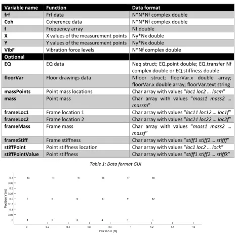
[image:22.595.74.526.250.590.2]

As a test case a table, see Figure 13, in the lab was used. On this table 18 locations where marked

according the grid in Figure 14. For this setup all frfs and vibration levels where measured using

SpecTest. From these measurements the matrices where tried to be derived using the methods from

Chapter 3. The Matlab script for this can be found in Appendix L.

(23)

[image:23.595.75.491.134.312.2]

Page 23 of 151

Figure 14: Table grid

In Figure 15 top left the co-located transfers are plotted from the measurements of the table. One can

see a distinctive resonance peak at 58Hz. This peak should therefore be visible in all estimation

methods or else it is not a good method.

Figure 15: Table Co-located transfers

[image:23.595.89.508.379.712.2]

(24)

Page 24 of 151

the resonance peak is at the wrong location. Therefore it can be concluded that this method does not

work on a real system.

The second method works significantly better as can be seen from the co-located transfer in Figure 15

bottom left. However the peak is still not at the correct location and also there is a lot unexpected

dynamic behaviour. Thus is concluded that this method does not lead to good results on a real system.

With final method, see Figure 15 bottom right

Error! Reference source not found.

, shows less u

nexpected dynamic behaviour. But the peak is still not at the correct location so this method also not

works on a real system.

(25)

Page 25 of 151

Chapter 6 Conclusions and

recommendations

6.1.1 Conclusions

The GUI made works well, the user can easily see how the floor would react to an altered situation.

Also the vibration levels can be obtained for the altered situation. Although the GUI is a great insight

tool, the placement for the EQ is still difficult since it is still not automated and the results dependent

on a lot of variables, e.g. disturbance source locations and local stiffness. When placing EQs one will

want to place as few as possible to cut cost, but also one needs to get the vibration levels within

specification.

6.1.2 Recommendations

The main recommendations for are

1. Run an experiment to test if the disturbance location estimation works

2. Retuning of tunable EQs

3. Automatization of EQ placement or a procedure

4. Loading of vibration levels specification

5. Adding of point damper and damper parameter to frame

6.1.3 Experiment

In the GUI the disturbance forces are estimated from the frfs and vibration levels with

𝐹

𝑑

= 𝑓𝑟𝑓

−1

∗ 𝑥

𝑑

It would be best to check if this idea also works on a real system. A simple way to do this is by making

a system with a known disturbance source, for instance a shaker. From the measurements of this real

system one should be able to reconstruct the disturbance force. A beginning was made with this

experiment but it has not proven to be successful. This is most likely due to not syncing of the phase.

Since there are more measurement points then sensors the vibration level measurement have to take

place in multiple measurements. To sync the phase the multiple experiments should have a common

sensor the measure the phase shift between measurements.

6.1.4 Retuning of tunable EQs

At the moment when a tunable EQ is placed it cannot be changed but it can be deleted. So if one

wants to adjust a tunable EQ one has to delete it and rebuild it from scratch. Also one cannot see how

the original EQ was constructed. Therefore it would be best if the original EQ could be loaded and

adjusted.

6.1.5 Automatization of EQ placement or a procedure

(26)

Page 26 of 151

where the floor vibration levels are above specification. Although the last points does not need to

have to any vibration entry points but due to large transfers can become above specification.

6.1.6 Loading of vibration levels specification

At the moment it is up to the user if the vibration levels specification are met. Therefore it would be

best to be able to load the specifications into the GUI. Also when this is added it would be best to also

give the user cues when the specifications are met and which locations are out of bounds.

6.1.7 Adding of point damper and damper parameter to frame

(27)

Page 27 of 151

References

[1]

S. Bank, Active Vibration Solutions, Eindhoven: Precisiebeurs, 2017.

[2]

R. Giesen, “Modal analysis techniques for (damped) floors,” 2017.

[3]

C. Felippa, “Introduction to Aerospace Structures,” 16 August 2017. [Online]. Available:

https://www.colorado.edu/engineering/CAS/courses.d/Structures.d/Home.html. [Accessed 2 Juli

2018].

[4]

J. Schilder, “Reader Dynamics 3 Flexible multibody dynamics,” p. 98.

[5] F. Koopman, Manual: Floor dynamics and vibration GUI V2, Enschede: MECAL, 2018.

[6]

Skorkmaz,

“wikimedia,”

9 December

2011.

[Online].

Available:

https://commons.wikimedia.org/wiki/File:Closed_Loop_Block_Deriv.png. [Accessed 9 July 2018].

[7]

“MECAL,” 2015. [Online]. Available: mecal.eu. [Accessed 9 July 2018].

[8]

“MECAL

High-tech/Systems,”

2015.

[Online].

Available:

http://www.mecal.eu/high-tech#hightechsystemdevelopment. [Accessed 9 July 2018].

(28)

Page 28 of 151

Appendix A

MECAL

MECAL [7] is founded in 1989 and the name MECAL comes from (

ME

chanical

CAL

culation). MECAL focussed

in the past on providing strength calculations and dynamic simulations performed on structures The plan

was to build a company with at most a dozen employees working in the consultancy sector. The company

was very focused on the competency and didn’t have a specific market orientation, so they would take on

any assignments or projects. But MECAL grew and became aware that it wasn’t possible to be specialized in

every field, so MECAL needed to specify. The conclusion was that MECAL strongly manifested with its

knowledge in two segments, namely the Wind and Semiconductor Market.

[image:28.595.75.539.360.681.2]

MECAL organogram is displayed in Figure 16. This internship took place in Enschede under Hightech/ Systems

[8].

(29)

Page 29 of 151

Appendix B

Reflection

The time I spent at MECAL I have gained first-hand experience of the many aspects going in a project and the

general process. From this I learned what to expect later in my working life and what I want in it. This is a

valuable lesson that I learned during my 3 month internship.

Looking back at the beginning of my internship it was difficult to start since the assignment was not yet fixed.

Since it was unclear at that moment which direction this internship would take. However starting from the

work of previous intern I had several ideas to add my part in a better understanding and modelling the

dynamics of floors.

From my supervisor I learned a lot about dynamics, being more distrustful to strange results, and the

importance of good visualization.

During this internship I had the chance to put several things I learned during my study into practice. For

instance the getting the equation of motion for a system, system identification and Matlab programming.

Most of my time I spent in Matlab either programming or processing results, but I also spent some time in

the lab doing experiments and doing research.

Although there was a positive working atmosphere, my project was highly individual. Therefore I missed

working within a team. This would be something I do not want in my working life later.

I think I functioned well despite my personal problem of suffering from depression. I do not think that this

had a vast impact on my internship as in it was mostly only noticeable when I was away for counselling.

(30)

Page 30 of 151

Appendix C

Matlab floor insight GUI code 2D

Version

The function below uses the function circular_arrow [9].

function twoD_floor_gui()

% twoD_floor_gui() %

% UI function to calculate mode shapes and

% Operating Deflection Shapes(ODS)of a two-dimensional floor % under force loading and with Equalizer

% The floor has only a length, not width, and can move only in z and % theta. Forces only in z direction and stiffness in theta

%

% INPUT:

% for modal plots needed

% N : number of beam elements

% kmid : approx. stiffness mid floor of only floor = 4k/N [N/m]

% kez : edge stiffness between wall an first/last mass in z direction [N/m]

% ketheta : edge stiffness between wall an first/last mass in theta direction [Nm/rad] % mtot : total mass floor [kg]

%

% derived param's

% Ke : element stiffness matrix

% m : mass of each indiv. mass element = mtot/N [kg] % Me : element mass matrix

% K : global stiffness matrix % M : global mass matrix %

% for ODS also needed

% cez : dampingconstant between edge and first element in z [-] % cetheta : dampingconstant between edge and first element in theta [-] % cz : damping between mass elements [-] cz = sqrt(m*k)/q [N/(m/s)]

% ctheta : damping between mass elements [-] ctheta = sqrt(m*k)/q [Nm/(rad/s)] % fods : disturbance frequency [Hz]

% Fdp : array with applied disturbance forces nodes (for ODS only) % FdA : array with applied disturbance forces amplitude (for ODS only) % Mdp : array with applied disturbance moments nodes (for ODS only) % MdA : array with applied disturbance moments amplitude (for ODS only) %

% for EQUALIZED ODS also needed

% EQ_Ptsz : z nodes which are equalized

% EQ_Ptstheta : theta nodes which are equalized %

(31)

Page 31 of 151 % || - - - ... - - - ||

%

% with || = wall, - = element %

% Z = array with Z positions for mass 1..N % only Z movement is allowed by the springs %

%

% OUTPUT:

% resonance frequencies

% mode shapes visualized in a plot % ODS

%

% METHOD

% (-1*lbd*M + K)*Z = F % with lbd = w^2 and -1 = i^2

% eigen freq and mode shapes follow from the determinant % of the dynamic matrix: D = K-lbd*M

% this can be computed with the eig(K,M) function in Octave/Matlab %

% For the ODS the follwing formula holds: % (-w^2*M+iw*C +K)*Z = F

% with C being the damping matrix

% Z movements can be calculated by Z = ( )\F %

% For the Equalized ODS:

% - the collocated percieved stiffness is calculated % compliance = K\F, stiffn = 1/compliance(i)

% - A stiffness (to earth) is added to the stiffness marix K

% which is 10 times greater than the perceived stiffness at that point % and frequency.

% this is the same as Sensitivity = 10 % K(i,i) = K(i,i) + stiffn

% Mark that the order in which points are being equalized is not trivial %

% ver 1 fkoo 3-7-2018

close all

global h;

% Define input parameters and UI

h.fig1 = figure('position',[10 10 1200 800],'name','TwoD floor GUI'); % button Calc

h.but= uicontrol('style','pushbutton','position', [10 10 60 40 ],'string','calc!'); set(h.but,'Callback',@CalcCallback);

% edit box N and text 'N'

h.t1 = uicontrol('style', 'text','position',[ 10 750,60,30],'string','N '); h.edN = uicontrol('style','edit', 'position',[ 80,750,60,30],'string','10'); % edit box and text kmid

h.t2 = uicontrol('style', 'text','position',[ 10 720,60,30],'string','kmid'); h.edkmid = uicontrol('style','edit', 'position',[ 80,720,60,30],'string','4e8'); % edit box and text kez

(32)

Page 32 of 151 h.edkez = uicontrol('style','edit', 'position',[ 80,690,60,30],'string','1.5e8');

% edit box and text ketheta

h.t4 = uicontrol('style', 'text','position',[ 10 660,60,30],'string','ketheta '); h.edketheta = uicontrol('style','edit', 'position',[ 80,660,60,30],'string','1.5e8'); % edit box and text m

h.t5 = uicontrol('style', 'text','position',[ 10 630,60,30],'string','mtot'); h.edm = uicontrol('style','edit', 'position',[ 80,630,60,30],'string','1.3e5'); % axes for modal plot

%h.ax1 = axes('units','pixels','position',[ 180,50, 1000,700]); %get(h.ax1,'position')

h.t6 = uicontrol('style', 'text','position',[ 10 560,60,30],'string','cz '); h.edqz = uicontrol('style','edit', 'position',[ 80,560,60,30],'string','1'); h.t7 = uicontrol('style', 'text','position',[ 10 530,60,30],'string','ctheta '); h.edqtheta = uicontrol('style','edit', 'position',[ 80,530,60,30],'string','1'); h.t8 = uicontrol('style', 'text','position',[ 10 500,60,30],'string','cez '); h.edqez = uicontrol('style','edit', 'position',[ 80,500,60,30],'string','3'); h.t9 = uicontrol('style', 'text','position',[ 10 470,60,30],'string','cetheta '); h.edqetheta = uicontrol('style','edit', 'position',[ 80,470,60,30],'string','3'); h.t10 = uicontrol('style', 'text','position',[ 10 440,60,30],'string','f ods '); h.edfods = uicontrol('style','edit', 'position',[ 80,440,60,30],'string','17'); % disturbance forces

h.t11 = uicontrol('style', 'text','position',[ 10 400,120,20],'string','define disturbance'); h.t12 = uicontrol('style', 'text','position',[ 10 370,60,30],'string','nodes z force'); h.edFdp = uicontrol('style','edit', 'position',[ 80,370,60,30],'string','1');

h.t13 = uicontrol('style', 'text','position',[ 10 340,60,30],'string','Amplitude (N) '); h.edFdA = uicontrol('style','edit', 'position',[ 80,340,60,30],'string','1');

h.t14 = uicontrol('style', 'text','position',[ 10 310,60,30],'string','nodes theta moment'); h.edMdp = uicontrol('style','edit', 'position',[ 80,310,60,30],'string','');

h.t15 = uicontrol('style', 'text','position',[ 10 280,60,30],'string','Amplitude (Nm)'); h.edMdA = uicontrol('style','edit', 'position',[ 80,280,60,30],'string','');

% EQUALIZER points

h.t16 = uicontrol('style', 'text','position',[ 10 240,120,20],'string','define EQ. nodes'); h.t17 = uicontrol('style', 'text','position',[ 10 210,60,20],'string','z nodes');

h.edPtsz = uicontrol('style','edit', 'position',[ 80,210,60,30],'string','2 3'); h.t18 = uicontrol('style', 'text','position',[ 10 180,60,20],'string','theta nodes'); h.edPtstheta = uicontrol('style','edit', 'position',[ 80,180,60,30],'string','');

% calculation is done in the function CalcCallback

end % function OneD_floor_gui

function CalcCallback(~,~)

global h; % handle to figure

% input for modeshapes

N = str2num(get(h.edN,'string')); kmid = str2num(get(h.edkmid,'string')); kez = str2num(get(h.edkez,'string'));

(33)

Page 33 of 151 m = str2num(get(h.edm,'string'));

me = m/N;

% Element matricies

Ke=kmid*N^3/48*[12 6 -12 6 ; 6 4 -6 2 ; -12 -6 12 -6 ; 6 2 -6 4]; Me=me/420*[156 22 54 -13 ; 22 4 13 -3 ; 54 13 156 -22 ; -13 -3 -22 4];

% input for ODS

cz = str2num(get(h.edqz,'string'));

ctheta = str2num(get(h.edqtheta,'string')); cez = str2num(get(h.edqez,'string'));

cetheta = str2num(get(h.edqetheta,'string')); fods = str2num(get(h.edfods,'string'));

% Distrubance forces Fd = zeros(2*N+2,1);

edFdp = str2num(get(h.edFdp,'string')); edFdA = str2num(get(h.edFdA,'string')); Fd(2*edFdp-1)=edFdA;

% Distrubance moments

edMdp = str2num(get(h.edMdp,'string')); edMdA = str2num(get(h.edMdA,'string')); Fd(2*edMdp)=edMdA;

% check dat Fd niet per ongeluk te groot wordt

if length(Fd) > 2*N+2 Fd = Fd(1:2*N);

end

% EQ points

edPtsz = str2num(get(h.edPtsz,'string'));

edPtstheta = str2num(get(h.edPtstheta,'string'));

EQ_Pts = sort([2*edPtsz-1 2*edPtstheta]); dx = 1/(N);

x = linspace(dx,1-dx,N+1); xleft = [0 dx];

xright = [1-dx 1];

% FILL in the modal masses M and K M= zeros(2*N+2,2*N+2);

K=M;

for i = 1:N

M(2*i-1:2*i+2,2*i-1:2*i+2) = M(2*i-1:2*i+2,2*i-1:2*i+2) + Me; K(2*i-1:2*i+2,2*i-1:2*i+2) = K(2*i-1:2*i+2,2*i-1:2*i+2) + Ke;

end

K(1,1) = K(1,1)+kez; K(2,2) = K(2,2)+ketheta;

(34)

Page 34 of 151 % compute eigen freq and mode shapes with magical eig function

[v,lbd] = eig(K,M); fres=zeros(1,length(lbd));

for i = 1:length(lbd)

fres(i) = sqrt(lbd(i,i))/(2*pi);

end

% plot first 6 (if available) modes on separate figure nplt = min(6,length(lbd));

for i = 1:nplt

subplot(nplt,3,3+3*(i-1)); hold off;

a = v(:,i)/v(1,i);

% eerst andere kant op in grijs plot(x,-a(1:2:end-1),'-o','color',

[0.7,0.7,0.7],'linewidth',4,'markersize',8,'markerfacecolor',[0.7,0.7,0.7]); hold on; % the masses with k's

plot(xleft,[0 -a(1)],'color',[.5,0.5,1],'linewidth',5); % left end plot(xright,[-a(end-1),0],'color',[.5,0.5,1],'linewidth',5); % right end % dan ene kant op

plot(x,a(1:2:end-1),'-ok','linewidth',4,'markersize',10,'markerfacecolor','k'); hold on; % the masses with k's

plot(xleft,[0 a(1)],'color',[0,0,0.8],'linewidth',5); % left end plot(xright,[a(end-1),0],'color',[0,0,0.8],'linewidth',5); % right end plot ([0,0],[-.5 .5],'k','linewidth',8); % wall

plot ([1,1],[-.5 .5],'k','linewidth',8); % wall plot([0 1],[0 0],'k');

xlim([0 1]);ylim([-1.2*max(abs(a)) 1.2*max(abs(a))]);

text(0.3,2*max(abs(a)),['res freq = ' num2str(fres(i)) 'Hz']); set(gca,'visible','off');

end

% ODS

% Fill in the C matrix

% elements C matrix Ce=zeros(4);

Ce(1:2:3,1:2:3)=[cz -cz;-cz cz];

Ce(2:2:4,2:2:4)=[ctheta -ctheta;-ctheta ctheta];

C=zeros(2*N+2,2*N+2);

for i = 1:N

C(2*i-1:2*i+2,2*i-1:2*i+2) = C(2*i-1:2*i+2,2*i-1:2*i+2) + Ce;

end

C(1,1) = C(1,1)+cez; C(2,2) = C(2,2)+cetheta;

(35)

Page 35 of 151 % Now calculate the deflection shape

w = 2*pi*fods;

D = -w^2*M + 1i*w*C+K; Z = D\Fd;

% Plot the ODS

% because not all masses move either the same way or the opposite way % we need to take into account the phase.

% We do this by plotting different points in time ( = different values for the phase) hods(1)= subplot(2,6,[2,3,4]);

hold off;

scalingy = 0.5/max(abs(Z(1:2:end-1))); scalingF = 0.5/max(Fd);

plot([0 1],[0 0],'k'); hold on; % 0 -line

for i = 1:N+1

% plot applied forces if Fd(2*i-1) ~= 0

plot([x(i) x(i)],[0 0.4*scalingF*Fd(2*i-1)],'r','linewidth',3); end % if

% plot applied moments if Fd(2*i) ~= 0

circular_arrow(gcf,0.1*scalingF*Fd(2*i),[x(i) 0],0,170,-1,'r'); end % if

end % for % boundary

% plot(x,abs(Z),'.-','color',[0.6 0.5 0.6],'linewidth',2); % plot(x,-abs(Z),'.-','color',[0.6 0.5 0.6],'linewidth',2);

Nl = 5; % number of lines in the plot 36 for each 10 degrees phi = [-1.5*pi,-pi,-pi/2,-pi/4,-pi/8];

for i = 1: Nl

plot(x,scalingy*abs(Z(1:2:end-1)).*cos(phi(i)+angle(Z(1:2:end-1))),'-o','color', [1-i/(1.3*Nl),1-i/(1.3*Nl),1-i/(1.3*Nl)],'linewidth',4);

hold on;

plot([0 dx],scalingy*[0 abs(Z(1)).*cos(phi(i)+angle(Z(1)))],'color' ,[1-i/(1.3*Nl),1-i/(1.3*Nl),1],'linewidth',4);

plot([1-dx 1],scalingy*[abs(Z(end-1)).*cos(phi(i)+angle(Z(end-1))) 0],'color' ,[1-i/(1.3*Nl),1-i/(1.3*Nl),1],'linewidth',4);hold on;

end

%plot(x,abs(Z).*cos(angle(Z)),'-o','color', [0 0 0 ],'linewidth',4);

%plot([1-dx 1],[abs(Z(N)).*cos(angle(Z(N))) 0],'color',[0,0,1],'linewidth',4); %plot([0 dx],[0 abs(Z(1)).*cos(angle(Z(1)))],'color',[0,0, 1],'linewidth',4);

% test with animation, plot only first moment, phi = 0 phi = 0;

h1= plot(x,scalingy*abs(Z(1:2:end-1)).*cos(phi+angle(Z(1:2:end-1))),'-ok', 'linewidth',4); h2 = plot([0 x(1)],scalingy*[0 abs(Z(1))*cos(phi+angle(Z(1)))],'-b','linewidth',4);

(36)

Page 36 of 151 ylim([-0.5,0.5]);

plot ([0,0],[-0.5/3 0.5/3],'k','linewidth',8); % wall plot ([1,1],[-0.5/3 0.5/3],'k','linewidth',8); % wall

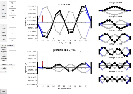
title(['ODS for ' num2str(fods) 'Hz']);

ylabel('Z position [m]'); xlabel('rel. X position [-]'); set(gca,'YTick',linspace(-0.5,0.5,10));

set(gca,'YTickLabel',linspace(-1/scalingy,1/scalingy,10)); Zorig= Z; % keep track of original movement

% Now calc forces needed for EQ

for i =1: length(EQ_Pts)

pt= EQ_Pts(i); % point to equalize %zpt = Z(pt); % movement of that point

Fhlp = zeros(2*N+2,1); Fhlp(pt) =1; % F for collocated stiffness Zcol = D\Fhlp; % collocated compl. z/F for point pt for f=fods;

keq = 10/Zcol(pt); % 10 times complex stiffness %10/abs(Zcol(pt)); % equivalent stiffness of active eq

K(pt,pt) = K(pt,pt) +keq;

end

% calculate new system ( with changed K matrix) D = -w^2*M + 1i*w*C+K;

Z = D\Fd; % calc new resulting movement

% now plot

hods(2) = subplot(2,6,[8,9,10]); linkaxes(hods,'y');

hold off;

plot([0 1],[0 0],'k'); hold on;% 0 -line

for i = 1:N+1

% plot applied forces if Fd(2*i-1) ~= 0

plot([x(i) x(i)],[0 0.4*scalingF*Fd(2*i-1)],'r','linewidth',3); end % if

% plot applied moments if Fd(2*i) ~= 0

circular_arrow(gcf,0.1*scalingF*Fd(2*i),[x(i) 0],0,170,-1,'r'); end % if

end % for

scalingy = 0.5/max(abs([Z(1:2:end-1);Zorig(1:2:end-1)])); % boundary

plot(x,scalingy*abs(Z(1:2:end-1)),'.-','color',[0.6 0.5 0.6],'linewidth',2); plot(x,-scalingy*abs(Z(1:2:end-1)),'.-','color',[0.6 0.5 0.6],'linewidth',2); Nl = 5; % number of lines in the plot 36 for each 10 degrees

phi = [-1.5*pi,-pi,-pi/2,-pi/4,-pi/8];

for i = 1: Nl

h5= plot(x,scalingy*abs(Z(1:2:end-1)).*cos(phi(i)+angle(Z(1:2:end-1))),'-o','color', [1-i/(1.3*Nl),1-i/(1.3*Nl),1-i/(1.3*Nl)],'linewidth',4);

hold on;

(37)

Page 37 of 151 h7 =plot([1-dx 1],scalingy*[abs(Z(end-1)).*cos(phi(i)+angle(Z(end-1))) 0],'color' ,[1-i/(1.3*Nl),1-i/(1.3*Nl),1],'linewidth',4);hold on;

end

plot(x,scalingy*abs(Z(1:2:end-1)).*cos(angle(Z(1:2:end-1))),'-o','color', [0 0 0 ],'linewidth',4); plot([0 dx],scalingy*[0 abs(Z(1)).*cos(angle(Z(1)))],'color',[0,0, 1],'linewidth',4);

plot([1-dx 1],scalingy*[abs(Z(end-1)).*cos(angle(Z(end-1))) 0],'color',[0,0,1],'linewidth',4);

ylim([-0.5,0.5]);

plot ([0,0],[-0.5/3 0.5/3],'k','linewidth',8); % wall plot ([1,1],[-0.5/3 0.5/3],'k','linewidth',8); % wall

title(['EQUALIZED ODS for ' num2str(fods) 'Hz']); ylabel('Z position [m]'); xlabel('rel. X position [-]'); set(gca,'YTick',linspace(-0.5,0.5,10));

set(gca,'YTickLabel',linspace(-1/scalingy,1/scalingy,10));

% Now animate!

for i = 1: 80 phi = i*2*pi/40; pause(0.15);

set(h1,'ydata',scalingy*abs(Zods(1:2:end-1)).*cos(phi+angle(Zods(1:2:end-1)))); set(h2 ,'ydata',scalingy*[ 0 abs(Zods(1)).*cos(phi+angle(Zods(1)))]);

set(h3 ,'ydata',scalingy*[ abs(Zods(end-1)).*cos(phi+angle(Zods(end-1))) 0]);

set(h5,'ydata', scalingy*abs(Z(1:2:end-1)).*cos(phi+angle(Z(1:2:end-1)))); set(h6, 'ydata',scalingy*[0 abs(Z(1)).*cos(phi+angle(Z(1)))]);

set(h7, 'ydata',scalingy*[abs(Z(end-1)).*cos(phi+angle(Z(end-1))) 0]);

end

(38)

Page 38 of 151

Appendix D

Matlab floor insight GUI code 2D

Version with floor parameters

The function below uses the function circular_arrow [9].

function twoD_floor_gui_floorParameters()

% twoD_floor_gui() %

% UI function to calculate mode shapes and

% Operating Deflection Shapes(ODS)of a two-dimensional floor % under force loading and with Equalizer

% The floor has only a length, not width, and can move only in z and % theta. Forces only in z direction and stiffness in theta

%

% INPUT:

% for modal plots needed

% N : number of beam elements % E : yield modulus [Pa]

% I : second moment of area [m^4] % L : floor length [m]

% kez : edge stiffness between wall an first/last mass in z direction [N/m]

% ketheta : edge stiffness between wall an first/last mass in theta direction [Nm/rad] % mtot : total mass floor [kg]

%

% derived param's

% Ke : element stiffness matrix

% m : mass of each indiv. mass element = mtot/N [kg] % Me : element mass matrix

% K : global stiffness matrix % M : global mass matrix %

% for ODS also needed

% cez : dampingconstant between edge and first element in z [-] % cetheta : dampingconstant between edge and first element in theta [-] % cz : damping between mass elements [-] cz = sqrt(m*k)/q [N/(m/s)]

% ctheta : damping between mass elements [-] ctheta = sqrt(m*k)/q [Nm/(rad/s)] % fods : disturbance frequency [Hz]

% Fdp : array with applied disturbance forces nodes (for ODS only) % FdA : array with applied disturbance forces amplitude (for ODS only) % Mdp : array with applied disturbance moments nodes (for ODS only) % MdA : array with applied disturbance moments amplitude (for ODS only) %

% for EQUALIZED ODS also needed

% EQ_Ptsz : z nodes which are equalized

% EQ_Ptstheta : theta nodes which are equalized %

(39)

Page 39 of 151 %

% || - - - ... - - - || %

% with || = wall, - = element %

% Z = array with Z positions for mass 1..N % only Z movement is allowed by the springs %

%

% OUTPUT:

% resonance frequencies

% mode shapes visualized in a plot % ODS

%

% METHOD

% (-1*lbd*M + K)*Z = F % with lbd = w^2 and -1 = i^2

% eigen freq and mode shapes follow from the determinant % of the dynamic matrix: D = K-lbd*M

% this can be computed with the eig(K,M) function in Octave/Matlab %

% For the ODS the follwing formula holds: % (-w^2*M+iw*C +K)*Z = F

% with C being the damping matrix

% Z movements can be calculated by Z = ( )\F %

% For the Equalized ODS:

% - the collocated percieved stiffness is calculated % compliance = K\F, stiffn = 1/compliance(i)

% - A stiffness (to earth) is added to the stiffness marix K

% which is 10 times greater than the perceived stiffness at that point % and frequency.

% this is the same as Sensitivity = 10 % K(i,i) = K(i,i) + stiffn

% Mark that the order in which points are being equalized is not trivial %

% ver 1 fkoo 3-7-2018

close all

global h;

% Define input parameters and UI

h.fig1 = figure('position',[10 10 1200 800],'name','TwoD floor GUI with parameters'); % button Calc

h.but= uicontrol('style','pushbutton','position', [10 10 60 40 ],'string','calc!'); set(h.but,'Callback',@CalcCallback);

% edit box N and text 'N'

h.t1 = uicontrol('style', 'text','position',[ 10 750,60,30],'string','N '); h.edN = uicontrol('style','edit', 'position',[ 80,750,60,30],'string','10'); % edit box and text E

(40)

Page 40 of 151 h.t3 = uicontrol('style', 'text','position',[ 10 690,60,30],'string','I');

h.I = uicontrol('style','edit', 'position',[ 80,690,60,30],'string','0.1'); % edit box and text L

h.t4 = uicontrol('style', 'text','position',[ 10 660,60,30],'string','L'); h.L = uicontrol('style','edit', 'position',[ 80,660,60,30],'string','20'); % edit box and text kez

h.t5 = uicontrol('style', 'text','position',[ 10 630,60,30],'string','kez '); h.edkez = uicontrol('style','edit', 'position',[ 80,630,60,30],'string','1.5e8'); % edit box and text ketheta

h.t6 = uicontrol('style', 'text','position',[ 10 600,60,30],'string','ketheta '); h.edketheta = uicontrol('style','edit', 'position',[ 80,600,60,30],'string','1.5e8'); % edit box and text m

h.t7 = uicontrol('style', 'text','position',[ 10 570,60,30],'string','mtot'); h.edm = uicontrol('style','edit', 'position',[ 80,570,60,30],'string','1.3e5'); % axes for modal plot

%h.ax1 = axes('units','pixels','position',[ 180,50, 1000,700]); %get(h.ax1,'position')

h.t8 = uicontrol('style', 'text','position',[ 10 520,60,30],'string','cz '); h.edqz = uicontrol('style','edit', 'position',[ 80,520,60,30],'string','1'); h.t9 = uicontrol('style', 'text','position',[ 10 490,60,30],'string','ctheta '); h.edqtheta = uicontrol('style','edit', 'position',[ 80,490,60,30],'string','1'); h.t10 = uicontrol('style', 'text','position',[ 10 460,60,30],'string','cez '); h.edqez = uicontrol('style','edit', 'position',[ 80,460,60,30],'string','3'); h.t11 = uicontrol('style', 'text','position',[ 10 430,60,30],'string','cetheta '); h.edqetheta = uicontrol('style','edit', 'position',[ 80,430,60,30],'string','3'); h.t12 = uicontrol('style', 'text','position',[ 10 400,60,30],'string','f ods '); h.edfods = uicontrol('style','edit', 'position',[ 80,400,60,30],'string','17'); % disturbance forces

h.t13 = uicontrol('style', 'text','position',[ 10 360,120,20],'string','define disturbance'); h.t14 = uicontrol('style', 'text','position',[ 10 330,60,30],'string','nodes z force'); h.edFdp = uicontrol('style','edit', 'position',[ 80,330,60,30],'string','1');

h.t15 = uicontrol('style', 'text','position',[ 10 300,60,30],'string','Amplitude (N) '); h.edFdA = uicontrol('style','edit', 'position',[ 80,300,60,30],'string','1');

h.t16 = uicontrol('style', 'text','position',[ 10 270,60,30],'string','nodes theta moment'); h.edMdp = uicontrol('style','edit', 'position',[ 80,270,60,30],'string','');

h.t17 = uicontrol('style', 'text','position',[ 10 240,60,30],'string','Amplitude (Nm)'); h.edMdA = uicontrol('style','edit', 'position',[ 80,240,60,30],'string','');

% EQUALIZER points

h.t18 = uicontrol('style', 'text','position',[ 10 200,120,20],'string','define EQ. nodes'); h.t18 = uicontrol('style', 'text','position',[ 10 170,60,20],'string','z nodes');

h.edPtsz = uicontrol('style','edit', 'position',[ 80,170,60,30],'string','2 3'); h.t19 = uicontrol('style', 'text','position',[ 10 140,60,20],'string','theta nodes'); h.edPtstheta = uicontrol('style','edit', 'position',[ 80,140,60,30],'string','');

% calculation is done in the function CalcCallback

end % function OneD_floor_gui

function CalcCallback(~,~)

Design of a Matlab based graphical user interface for visualization and enhancement of floor dynamics

Internship report: Design of a Matlab

based graphical user interface for

visualization and enhancement of floor

dynamics

F.B.Koopman

s0166626

Document name: Report_fkoo.docx

Date: 23 July 2018

MECAL, Enschede, The Netherlands

Supervisor Mecal: Servaas Bank

Internship period: 1/5/2018-31/7/2018

University of Twente

Faculty of Engineering Technology

Internship report: Design of a Matlab based graphical

user interface for visualization and enhancement of

floor dynamics

Document name:

Report_fkoo.docx

Date:

23/07/18

Written by:

Frederik Koopman, MECAL, Enschede, The Netherlands

Reviewed by:

Servaas Bank, MECAL, Enschede, The Netherlands

Approved by:

Servaas Bank, MECAL, Enschede, The Netherlands

Document by:

MECAL, Enschede, The Netherlands

Mailing list:

MECAL (1x)

Pages incl. cover:

151

Keywords:

Floor vibrations, floor vibrations reduction, floor dynamics

Language:

English

Software version:

Microsoft Word 2016

Contributing Authors

Name Author

Part(s) of this document

Frederik Koopman

All

Document change and history record

Version

Date

Page (s)

Short description

1.0

23/07/18

151

First Issue

Summary

Table of contents

Summary ... 3

Preface and acknowledgements ... 6

Chapter 1 Introduction ... 7

1.1

Assignment description ... 7

1.2

Outline of the report ... 7

Chapter 2 Floor insight GUI ... 8

2.1

Existing version: 1D ... 8

2.2

First new version: 2D ... 9

2.3

Second new version: 2D with floor parameters ... 11

2.4

Third new version: 3D with floor parameters ... 11

2.5

Fourth new version: 3D with floor parameters and not square floors ... 12

Chapter 3 Floor model estimation ... 14

3.1

Higher DOF systems ... 14

3.2

Matrices estimation ... 15

Chapter 4 Matlab based GUI ... 17

4.1

_{Report_fkoo.docx}

_{MECAL, Enschede, The Netherlands}

_{MECAL (1x)}

₁₅₁

_{Floor vibrations, floor vibrations reduction, floor dynamics}

_English

_{Microsoft Word 2016}