MASTER THESIS
Investigation of the
Scope and Limitations of
Gradient Enhanced Crystal
Plasticity in Explaining
Macroscopic Phenomena
B. Nijhuis
Faculty of Engineering Technology (ET) Chair of Nonlinear Solid Mechanics
Exam committee:
Prof. dr. ir. A.H. van den Boogaard Dr. ir. E.S. Perdahcio˘glu
Dr. ir. T.C. Bor Ir. E.E. As¸ik Document number:
In a wide range of applications, it is important to be able to model the constitutive response of materials. Most models however fail to predict macroscopically observed phenomena in plastic deformation: the Hall-Petch effect, Bauschinger effect and anelastic behaviour. A gradient enhanced crystal plasticity model, in which slip gradients are incorporated in the hardening model through geometrically necessary dislocations (GNDs), is believed to include the physical basis to represent these phenomena. A com-prehensive review about its general applicability in this content is however not available. The aim of this work is therefore to assess the scope and limitations of a gradient enhanced crystal plasticity model in predicting macroscopic phenomena observed in plastic deformation of metals.
To establish a consistent simulation framework, a literature study is performed to determine the perquis-ites of calculating GND-densities in finite-strain problems. Calculations based on either referential or spatial slip gradients are found suitable for this purpose. This outcome is validated using dedicated sim-ulations, showing that the original gradient calculation algorithm can be retained. This code is extended for use with periodic boundary conditions.
Macroscopic phenomena are investigated by simulating the response of two-dimensional representative volume elements consisting out of hexagonally shaped grains under various loadings. The Hall-Petch ef-fect in work hardening is very well represented by the length scale that is introduced by the slip gradients. Including GNDs clearly extends the width of the stress distribution within the material. The presence of such a stress distribution results in small scale plasticity effects when the material is unloaded after de-formation. The Bauschinger effect is hereby enhanced. Small amounts of anelasticity are also observed as a result, but not as pronounced as experimentally observed.
The validity of the gradient enhanced crystal plasticity model is tested by a quantitative comparison of the evolution of GND-densities with experimental results. Using electron backscatter diffraction, local misorientations between material points can be characterised and related to the GND-density. The nature of both the density distribution as well as the evolution of the total GND-number with strain agree between experiments and simulations. The experimentally observed initial dislocation densities are not present within the numerical model though. Possibilities for including a realistic initial dislocation distri-bution should therefore be investigated.
As extension to the theoretical framework of the model, an alternative version for the included stress-update algorithm is proposed. The commonly applied check for elastic deformations is removed by modifying the flow criteria. It is shown it can be applied to problems involving small lattice rotations suc-cessfully but requires further research in maintaining a stable set of active slip systems in large-rotation problems.
This thesis describes the findings of the research I undertook in partial fulfilment of the requirements for the degree of Master of Science in Mechanical Engineering at the University of Twente. It is performed on the subject of crystal plasticity models, which are increasingly used in modelling the constitutive be-haviour of metals. The research started from my interest in modelling metal plasticity developed during my internship. During my graduation period from January to September 2018, I have been able to gain many new insights into the subject of crystal plasticity and a better understanding of the plastic beha-viour of metals in general. With this new understanding and the final result of this research I am very satisfied.
My work was supervised by dr. ir. E.S. Perdahcio˘glu, whom I would like to thank for formulating this challenging but rewarding assignment, his guidance and support throughout the research and providing me with the feedback that lead to this thesis. I would also like to express my gratitude to ir. E.E. A¸sik for supporting me with the simulations on many occasions and agreeing to take place in my graduation committee. His contribution to this thesis by performing the EBSD-measurements is greatly appreciated. I wish to thank the remaining members of my graduation committee, prof. dr. ir. A.H van den Boogaard and dr. ir. T.C. Bor for offering their time and effort in the final phase of my studies.
I would like to thank my friends and roommates for the pleasant time, fruitful discussions and support they offered during my graduation. A special word of thanks goes out to my family and girlfriend for their everlasting support, guidance and motivation that greatly helped me in completing this thesis.
Last but not least, I would like to thank you as reader for showing your interest in my work. Haaksbergen, September 2018,
1 Introduction 1
2 Constitutive framework of crystal plasticity 4
2.1 Kinematical model of crystal deformation . . . 4
2.2 Stress response . . . 5
2.3 Material behaviour in the plastic regime . . . 5
2.3.1 Hardening behaviour . . . 6
2.4 Algorithmic implementation . . . 8
2.4.1 Discretizing constitutive equations . . . 8
2.4.2 Stress update algorithm with elastic check and active set determination . . . 9
2.4.3 Gradient and GND-density calculations . . . 12
2.4.4 Finite Element implementation . . . 12
3 Extensions to the crystal plasticity model 14 3.1 Stress update algorithm without elastic check and active set determination . . . 14
3.1.1 Implementation of modified flow criteria in stress update algorithm . . . 15
3.1.2 Comparison of the algorithms . . . 16
3.2 Gradient calculations in periodic models . . . 18
3.2.1 Comparison of the gradient codes . . . 21
3.3 Determining GND-densities in a finite-strain formulation . . . 22
3.4 Conclusions and recommendations . . . 24
4 Verification of the crystal plasticity model 25 4.1 Verification of the lattice rotation update . . . 25
4.2 Verification of the finite strain implementation . . . 26
4.2.1 Conclusion . . . 28
5 Predicting macroscopic phenomena using a gradient-enhanced crystal plasticity model 29 5.1 Modelling aspects . . . 29
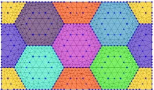
5.1.1 RVE with hexagonal grains . . . 30
5.2 The Hall-Petch effect . . . 31
5.2.1 The Hall-Petch effect in crystal plasticity models . . . 31
5.2.2 Setting up the FEM-models . . . 32
5.2.3 Results . . . 34
5.2.4 Discussion of results . . . 37
5.2.5 Conclusions . . . 39
5.3 The Bauschinger effect . . . 40
5.3.1 Setting up the FEM-models . . . 41
5.3.2 Results . . . 42
5.3.3 Discussion of results . . . 45
5.3.4 Conclusions and recommendations . . . 48
5.4 The anelasticity effect . . . 48
5.4.1 Setting up the FEM-models . . . 50
5.4.2 Results and discussion . . . 50
5.4.3 Conclusions and recommendations . . . 53
6 Experimental validation of the GND-evolution 54 6.1 Methods . . . 54
6.2 Results . . . 56
6.3 Discussion of results . . . 59
6.4 Conclusions and recommendations . . . 59
7 Conclusions 60
A Derivation of kinematical model assuming small elastic stretch 66
B Continuously differentiable approximation of the max() function 68
C Stress-update algorithm flowcharts 71
D Driver input files for future work 72
E Generating RVEs with random disorientation distributions 73
E.1 Generating random crystallographic orientations . . . 73 E.2 Calculating disorientation distributions . . . 74 E.3 RVEs with random disorientation distributions . . . 75
Modelling the constitutive response of materials is important in various stages in the lifetime of products. Whether it concerns the production and processing stage of raw materials, the transformation of raw materials into a final product or its usage phase, insight into the material’s response to applied loads and deformation aids in the design process, quantifying product characteristics and assessing possible modes of failure throughout each of these phases [1]. Implementation of constitutive models into simu-lation software makes it possible to account for material induced limitations on product performance in early stages of the design process, limiting rework costs and time.
To describe the evolution of (plastic) deformation within metals, two main aspects need to be taken into consideration. The onset of plastic flow is described by the material’s yield stress. After yielding and with increasing plastic flow, an increase in stress is observed: the material work-hardens. Thus, the apparent flow stress changes with ongoing deformation. The evolution of flow stress therefore needs to be taken into account by a suitable hardening model.
Different possibilities for implementing such behaviour in numerical models exist. The most elementary, but least general, method is a direct experimental characterisation of the response for the material and loading conditions that will be simulated. Generality, modifiability and implementability of this approach can be improved by using mathematical representations of stress-strain curves based upon a limited set of material parameters. However, the loading conditions that can be represented with conventional testing methods are limited. A wide variety of multi-axial yield criteria has therefore been developed to be able to extrapolate results from testing conditions to general stress states [2].
Even though plastic behaviour under arbitrary stress states can be captured using a suitable yield-criterion and hardening function, some macroscopic phenomena commonly observed in plastic deform-ation of metals are difficult to implement in continuum models [3]. These include the Bauschinger and anelasticity effects in processes where the loading direction is changed and grain-size dependency of material properties, the Hall-Petch effect. Numerous attempts have been made to account for this short-coming by extending phenomenological continuum models. The main disadvantage of these models is the increasing number of fitting constants and empirical extensions underlying them [4].
The physical origin of the abovementioned macroscopic effects is often related to microstructural in-homogeneities inherent to polycrystalline materials. Within a polycrystalline aggregate, each grain has a distinct lattice direction and is mechanically anisotropic [5]. Together with the requirement of continu-ity of the deformation of adjacent grains along their common boundaries, this causes inhomogeneous deformation within grains. With decreasing grain size, the level of inhomogeneity at the grain bound-aries increases [6] and it was hypothesized already in 1950 that this mechanism is responsible for a size-dependent macroscopic response [7]. Another effect that arises from lattice misorientations is the formation of residual stresses within the microstructure, which can be correlated to the macroscopically observed Bauschinger effect [8]. Anelasticity effects are another reflection of small scale plasticity ef-fects during unloading [9].
From the aforementioned observations, it becomes apparent that microstructural effects need to be taken into account to fully capture the constitutive response of metals. At the microscale, plastic de-formation can be modelled most suitably using crystal plasticity models [10]. Herein, plastic deformation is assumed to be caused solely by dislocation slip on the material’s individual slip systems. Since the method was first introduced in 1982 by Pierce et. al. [11], a growing interest in crystal plasticity finite element modelling has developed and it was used in a wide range of applications [5]. The macroscopic response of a polycrystalline material can be simulated using a crystal plasticity framework by means of a representative volume element (RVE). In such two- or three-dimensional models, a number of dif-ferently oriented grains is present. Macroscopic quantities are obtained from the RVE’s microscopic response under appropriate boundary conditions through averaging principles [12].
Results from crystal plasticity simulations performed using RVEs have shown that size-dependent ma-terial properties (e.g. [13–15]), the Bauschinger (e.g. [16,17]) and anelasticity effects (e.g. [18]) can be captured. In these results however, the formulations for the description of crystallographic slip are often modified or extended explicitly to add the intended macroscopic behaviour to the model. This leads to the same disadvantages pointed out for the extended continuum models above.
It would therefore be desirable to obtain a model that is capable of correctly capturing the macroscopic behaviour without explicit modifications to the underlying constitutive framework. This model should be based upon an experimentally justifiable, physical basis. In this work, such a model is hypothesised to be represented by a gradient enhanced crystal plasticity model. The reasoning behind this choice will now be discussed.
Consider the class of phenomenologically based crystal plasticity models, in which the evolution of slip and slip resistance is governed by the total dislocation densities on the slip systems ([5,12]). Here, a higher dislocation density implies a higher resistance against deformation. From a macroscopic point of view, it has long been agreed that it is possible to distinguish two types of dislocations [19]. Statistically stored dislocations (SSDs) form during uniform plastic deformation due to random trapping. Geomet-rically necessary dislocations (GNDs) on the other hand, form during inhomogeneous deformation to maintain compatibility of the lattice. The evolution of the SSD density can thus be expressed as function of slip [12]. As inhomogeneous plastic deformation is only possible if there exist gradients of plastic slip, the GND density can be expressed as function of slip gradients [20]. Through the incorporation of the GND density in the evolution equation of the slip resistance, a gradient-enhanced crystal plasticity model is obtained.
Due to differences in lattice orientations between adjacent grains in polycrystalline materials, GNDs primarily form near grain boundaries ([21,22]). With decreasing grain size, the level of inhomogeneity at the grain boundaries and thus the number of GNDs increases. Together with the length scale that is in-troduced by the Burgers vector that relates the slip gradients to GND-densities [6], a gradient-enhanced model crystal plasticity model is rendered size dependent. A better representation of the Hall-Petch effect is thus expected. The non-uniform distribution of GNDs over the grains will additionally cause non-uniform hardening and thus a widening of the stress distribution over the material. The Bauschinger and anelasticity effects resulting from microstructural residual stresses are therefore anticipated to be-come more pronounced when including GNDs.
Literature results published on applications of gradient enhanced crystal plasticity methods so far, are generally limited to a single macroscopic phenomenon. Both rate-dependent and rate-independent im-plementations are used and great differences are found in the formulation of slip system hardening. Additionally, the results differ in terms of simulated material and RVE setup. Also, two- and three-dimensional models are used, with realistic as well as conceptual microstructures. Therefore, a good indication of the overall applicability of gradient enhanced crystal plasticity in predicting macroscopic phenomena in plastic deformation is not available, as results are not comparable.
Within this work, it is strived to overcome this shortcoming in the published literature. The full range of macroscopic phenomena mentioned above will be simulated using the same crystal plasticity model and RVEs that are similar in setup. No extensions or modifications to the constitutive formulation of crys-tal plasticity will be made apart from the inclusion of gradient effects through GNDs and the hardening model. The formulation is thus not adapted to fit one particular phenomenon. This provides insight into the extent to which the Hall-Petch, Bauschinger and anelasticity effects can be predicted by the pres-ence of GNDs and thus inhomogeneous plastic deformation within the microstructure.
If successful in representing the constitutive response of metals, GECP-models provide a versatile tool in material development and characterisation, based on well motived underlying physical mechanism. The final goal of this research is therefore to assess the general applicability of a gradient enhanced crystal plasticity model in capturing macroscopic phenomena observed in plastic deformation of metals.
The remainder of this report is structured in three parts. The first part concerns the theoretical aspect of the work. The description of the theory behind GECP-method and its implementation is described in Chapter2. Extensions to the current model are covered in Chapter3and its validation is discussed in Chapter 4. The second part is formed by the application of GECP to simulations of macroscopic phenomena in plasticity in Chapter5. The final part is dedicated to a qualitative experimental validation of the simulation results and is given in Chapter6.
The notations that will be used throughout this work are defined as follows. Bold capital letters denote tensors, bold lowercase letters denote vectors and lightface lowercase letters denote scalars. Given three second-order tensorsA,BandCand using Einstein’s summation convention, the single contrac-tion tensor product is written asA=BCwithCij =AikBkj. The dot-operator is omitted for readability. The double contraction tensor product is denoted using the colon operator as d = A : B = AijBij. The tensor product of two vectors m and nis defined as A = m⊗nwith Aij = minj. A−1 and AT represent the inverse and transpose of a tensorA, respectively. The gradient operator is used as
∇({•}) =∂({•})/∂x. Superscripts(α)and(β)denote properties of a slip systemαandβ, respectively.
crystal plasticity
Within this chapter, the constitutive relations underlying the gradient-enhanced crystal plasticity model used in this work will be introduced. In crystal plasticity models, plastic deformation is assumed to occur due to dislocation slip on slip systems in the crystal lattice. A kinematic model that relates this crystallographic slip to the deformation of the crystalline material is discussed in Section2.1. Based on this description, the constitutive relation between deformation and load is derived in Section 2.2. The material behaviour in the plastic regime, including the flow criteria and hardening behaviour, is further elaborated on in Section2.3. The algorithmic implementation of the crystal plasticty model is described in Section2.4.
2.1 Kinematical model of crystal deformation
Figure 2.1:Schematic overview of the multiplicative decompositionF=FeFp
The kinematical framework of finite-strain crystal plasticity models is commonly based on the multiplic-ative decomposition of the deformation gradient into an elastic and a plastic part, known as Kröner’s decomposition:
F=FeFp (2.1)
In crystal plasticity, plastic deformation is caused by shearing of given slip systems in the materials. This shear deformation is a result of dislocation movement through the crystal lattice [23]. As plastic flow due to dislocation movement does not change the lattice structure, the intermediate configuration ¯
Bdefined byFp is often assumed to leave the crystal lattice undistorted and unrotated. In this irrotational crystal plasticity formulation, the elastic part of the deformation accounts for all lattice distortions and rigid body rotations. A schematic overview of this decomposition is shown in Figure2.1.
The deformation of a crystal with n possibly active slip systems α ∈ [1,2, ..., n] can be obtained by summing slip contributions on individual systems. For large deformations, slips are not well defined
quantities, but slip ratesare. The plastic deformation of crystalline materials is therefore formulated in
terms of slip rates via the plastic velocity gradient [24]. As a result, the kinematical framework will be set up in terms of velocity gradients.
The plastic velocity gradient is defined as function of the slip ratesγ˙(α)by
Lp= n
X
α=1 ˙
γ(α)n(0α)⊗s(0α) (2.2)
where the slip-plane normal n(0α) and slip directions(0α) are constant vectors defined in the reference configuration. By noting that the resulting plastic deformation of a single slip step is small, the slip rates on individual slip systemsαmay be summed without taking into account the order of dislocation motion [5].
The total velocity gradient in the deformed configuration,L= ˙FF−1, can be additively decomposed into an elastic and a plastic part usingL=Le+Lp. The plastic velocity gradientLpis mapped to the current configuration by the elastic rotationReand the total velocity gradient is written as
L=Le+ReLpRTe (2.3)
Substitution of (2.2) into (2.3) then gives
L=Le+ n
X
α=1 ˙ γ(α)Re
n0(α)⊗s0(α)RTe =Le+ n
X
α=1 ˙
γ(α)Ren (α) 0
⊗Res (α) 0
=Le+ n
X
α=1 ˙
γ(α)n(α)⊗s(α) (2.4)
by the orthogonality ofRe. The deformation of the crystalline material is thus defined by the plastic slip on its various slip systems and elastic rotations of the crystal lattice. The formulation in (2.4) will be used to derive the constitutive relation for the crystal plasticity model in the subsequent section.
2.2 Stress response
Based on the result from (2.4), it can be seen that the deformation rate of a crystalline material can be decomposed into an elastic and a plastic part
D=De+Dp (2.5)
The plastic strain rate is given by the symmetric part of the plastic velocity gradient, Dp = sym (Lp). From the definition in (2.2), it is found that
Dp= n
X
α=1 ˙
γ(α)syms(α)⊗n(α)= n
X
α=1 ˙
γ(α)P(α) (2.6)
as expressed in the final configurationBand by definingP(α)as the symmetric part of the Schmid tensor s(α)⊗n(α).
The objective rate for the Cauchy stress is now given by
◦
σ=Ce:De=Ce: D− n
X
α=1 ˙ γ(α)P(α)
!
(2.7)
by usingDe=D−Dp.Ceis the isotropic elastic stiffness tensor. With this expression, the constitutive relation for a crystal plasticity model capable of describing large rotations and large plastic deformations has been defined.
2.3 Material behaviour in the plastic regime
As discussed before, the plastic behaviour of the material takes place at the slip system level. Therefore, the evolution of the slip rates in (2.2) needs to be defined. Similar to conventional plastic material models, plastic slip is allowed when the shear stress on a slip system reaches an initial flow stress: the critical resolved shear stress. Upon further deformation, the resistance against deformation increases: slip systems harden by an increasing critical resolved shear stress. It has to be noted that no slip occurs on a slip system prior to exceeding the flow stress.
The evolution of the slip rates can both be described by phenomenologically as well as microstructurally-based models [12,25]. For the first category of models, the critical resolved shear stress is updated as function of plastic slip. The latter category often uses a measure of the dislocation density within the material as internal variable to update the critical resolved shear stress. Within this work, a dislocation-density based crystal plasticity model will be used.
The flow behaviour of the slip systems is then governed by the flow criteria
φ(α)=τ(α)−τc(α)(ρ) (2.8)
in which the critical resolved shear stressτc(α)is a function of the dislocation densityρ. The resolved shear stress τ(α) on a slip system α can be found using the symmetric part of the Schmid tensor according to
τ(α)=σ:P(α) (2.9)
2.3.1 Hardening behaviour
Hardening of a slip system due to the evolution of the dislocation density in the material can be described by the Taylor model
τf =cµb
√
ρ (2.10)
whereτf is the flow stress, c is the Taylor factor, µis the shear modulus and b is the Burgers vector length. A primary slip system can harden directly due to the formation of dislocations during a slip event of this system. A non-active, secondary slip system may experience hardening because of the generated dislocations by the primary slip too. This phenomenon is referred to as latent hardening and can be included in the Taylor model by the introduction of an interaction matrixQ(αβ)as function of six independent coefficients Q(0αβ) ... Q(5αβ) [10, 12]. In addition to the dislocation-induced hardening, a constant initial flow stressτ0representing the Peierls Nabarro stress is included. The critical resolved shear stress on a systemαthen follows from the dislocation densities on all systemsβ by
τc(α)=τ0+cµb
v u u t
n
X
β=1
Q(αβ)ρ(β) (2.11)
Within a material, two types of dislocations can be distinguished. Statistically stored dislocations (SSDs) form during plastic deformation of the material by random trapping. When a crystal is subjected to in-homogeneous deformation, gradients of plastic slip arise. Geometrically necessary dislocations (GNDs) form as a result of such deformations in order to maintain compatibility in the crystal lattice. Following [10], the total dislocation density is calculated as
ρ(α)=ρSSD(α) +ρ(GNDα) (2.12)
Due to their dependence on gradients of plastic slip, the presence of GNDs introduces a length scale in the crystal plasticity model, which renders the model size-dependent. This size-dependency would not have been present if only SSDs were included in the hardening model. Additionally, the presence of GNDs introduces a source of a remaining, inhomogeneous plastic deformation upon load removal. This is caused by the formation of equally-signed dislocation arrangements of which the net dislocation sign does not cancel out at the continuum level, where this is the case for the SSD-population. As introduced before, it is for these two reasons that a gradient-enhanced crystal plasticity model is believed to be able to capture macroscopic phenomena such as the Hall-Petch, Bauschinger and anelasticity effects.
(a)Projection of∇γ(α)×n(α)onto slip system
geometry
(b)Accumulation of GNDs due to slip gradients in
s(α)-direction (top) andl(α)-direction (bottom) . Figure adapted from [26]
Figure 2.2:Relation between GNDs and curl of the plastic deformation gradient
Evolution of statistically stored dislocation densities
The evolution equation of the statistically stored dislocation density is given as function of the slip rates by
˙
ρ(SSDα) = γ˙ (α) γ∞
ρ∞SSD−ρ(SSDα) (2.13)
from which the value forρSSDas function of the plastic slip can be obtained [12]:
ρ(SSDα) =ρ∞SSD
1−
1−ρ
0 SSD ρ∞SSD
exp
−γ
(α) γ∞
(2.14)
Here, ρ0
SSD andρ∞SSD are the initial and saturation densities of statistically stored dislocations, respect-ively. The parameterγ∞determines the rate of saturation of the dislocation on the slip system.
Evolution of geometrically necessary dislocation densities
For the case of small deformation crystal plasticity, which is based on the additive decomposition of the deformation gradient
H=He+Hp (2.15)
the Burgers tensor is defined as [24]
G=CurlHp (2.16)
By assuming that the plastic distortion of a single crystal is solely caused by simple shear due to dislo-cation movement on given slip systems, the plastic deformation gradient can be written as
Hp=X α
γ(α)s(α)⊗n(α) (2.17)
wheres(α)is the slip direction andn(α)is the slip system normal. Substitution of (2.17) into (2.16) yields
G=X α
∇γ(α)×n(α)⊗s(α) (2.18)
which can be rewritten as [27] G=X
α
h
l(α)·∇γ(α)s(α)⊗s(α)−s(α)·∇γ(α)l(α)⊗s(α)i (2.19)
as apparent from Figure2.2a. The termsl(α)·∇γ(α)ands(α)·∇γ(α)actually represent projections of the slip gradient∇γ(α)on the slip system vectorsl(α) ands(α), respectively. As seen in Figure2.2b, a gradient of slip in the direction ofs(α)gives rise to an accumulation of edge dislocations, whereas a slip gradient inl(α)requires an accumulation of screw dislocations. Using the definitions
ρ(GNDα) ,=l(α)·∇γ(α)andρ(GNDα) ,`=−s(α)·∇γ(α) (2.20) the relation in (2.19) can thus be expressed in terms of the densities of geometrically necessary edge (`) and screw () dislocations following [26]
G=X α
h
ρ(GNDα) ,s(α)⊗s(α)+ρ(GNDα) ,`l(α)⊗s(α)i (2.21)
Defining the Burgers tensor as in (2.16), a relation between the gradient of plastic slip and the densities of geometrically necessary dislocation can thus be derived. For the case of small deformations, gradients may be defined in the undeformed configuration and the directions of the vectors s(α) and l(α) can be assumed to remain unchanged. This makes that the dislocation densities can be calculated in a straightforward manner once the distribution of plastic slips throughout the material is known.
2.4 Algorithmic implementation
The numerical implementation of the stress-update component of the crystal plasticity code discussed in this work is based on the formuations of [10, 23, 28]. Herein, a fully implicit formulation is used to solve for the plastic slip increments. This algorithm includes an elastic check and the set of active slip systems is determined iteratively. Within this section, an overview of the underlying formulation of the stress-update algorithm is given. The discretization of the constitutive equations that forms the basis for the stress-update algorithm is discussed in Section 2.4.1. The algorithmic implementation of this discretization to determine the final stress state in a crystalline material is described in Section2.4.2. The gradient computation procedure to determine the densities of GNDs in the material is outlined in Section2.4.3. An overview of the FEM-implementation of the algorithm is provided in Section2.4.4.
2.4.1 Discretizing constitutive equations
The basis for the formulation of a stress update algorithm is formed by discretizing the constitutive relations. The rate equation for the Cauchy stress in (2.7) is therefore rewritten in incremental form as
∆σ=Ce: ∆e=Ce: (∆−∆p) (2.22)
using the rate of deformation tensor D work-conjugate to the Cauchy stress to define the strain rate, ˙
=D. Integration of the plastic strain rate˙pfollowing the backward Euler method gives an expression for the plastic strain increment in terms of the plastic strain rate at the end of a step
∆p≈˙pn+1∆t (2.23)
in a fully implicit formulation. Insertion of the formulation of the flow rule ˙p = n
P
α=1 ˙
γ(α)P(α)into (2.23) yields the equation for the plastic strain increment
∆p= n
X
α=1 ˙
γn(α+1)∆tP(α)≈
n
X
α=1
∆γn(α+1)P(α) (2.24)
Substitution of (2.24) in (2.22) gives the implicit stress update formulation
σk+1=σk+ ∆σ=σ∗−Ce: n
X
α=1
∆γ(kα+1)P(α) (2.25)
where the trial stressσ∗is defined as
σ∗=σn+Ce: ∆n (2.26)
in which the strain increment ∆n is prescribed by the FEM-solver andσn is the previous equilibrium stress state of the material.
Based on the trial stress state and flow criteria values, either elastic or plastic deformation occurs. In the case of plasticity, accumulating plastic strain will affect the flow criteria due to hardening. This makes that in general, the expression for the stress update (2.25) has to be solved for using an iterative scheme. Two of such fully implicit schemes will be discussed in the remainder of this work.
2.4.2 Stress update algorithm with elastic check and active set determination
Miehe et. al. [28] have developed an implicit stress update algorithm in the constitutive framework of small strain single crystal plasticity. In the work of Soyarslan et. al. [10], it was extended to a finite-strain kinematical framework by including i.a. a lattice rotation update after a converged stress update step. The overall functioning of the stress update part of the code remains unchanged, however. Its implementation, together with the lattice rotation update will be described in this section. A flowchart of the algorithm is provided in TableC.2
Elastic check
Given the trial stress stateσ∗obtained from (2.26), the resolved trial shear stress on a slip systemαcan be calculated usingτ∗(α)=σ∗ :P(α). Based on the current value for the critical resolved shear stress τc,k(α), the flow criteria are evaluated in the elastic check
φ∗α=σ(α):P(α)−τc,n(α)<0 ∀α∈(1, ..., n) (2.27) If (2.27) is satisfied, the step is elastic. The returned tangent stiffness matrix is then set toCe and the final stress state equals the trial stress. Otherwise, plastic slip occurs and the Karush-Kuhn-Tucker conditions
∆γ(α)≥0, φ(α)≤0, ∆γ(α)φ(α)= 0 (2.28)
have to be satisfied. This is done using the following two steps.
Plastic slip update
The flow criteria are redefined in terms of the Cauchy stress as
r(α)≡φ(α)=σ:P(α)−τc(α)(ρ) (2.29)
Given a fixed setAof active slip systems, substitution of the expression of the stress at the end of the
increment, (2.25), into (2.29) yields the expression for the approximated consistency conditions ˜
r(α)=σ∗:P(α)−X
β∈A
∆γk(β+1)P(α):Ce:P(β)−τ (α)
c,k(ρ) = 0 (2.30)
For a fixed trial stress, (2.30) can be solved for the incremental plastic slips∆γ(α)using the linearisation
r(α)−B(αβ)∗∆γ(nβ+1) = 0 (2.31)
with the Jacobian matrix
B(αβ)∗≡ −∂r
(α) ∂γk(β+1)
=P(α):Ce:P(β)+ ∂τ (α) c
∂γ(kβ+1) (2.32)
Using (2.31) and (2.32), a Newton-Raphson scheme is employed to iteratively update the values for the plastic slip. To be able to do so, the derivative of the critical resolved shear stress with respect to the plastic slip needs to be determined. The critical resolved shear stress is governed by the hardening behaviour of the slip systems and thus a function of ρSSD andρGND. ρSSD is dependent on the plastic slip and the contribution
∂ρ(SSDα) ∂γk+1
= 1
γ∞ ρ ∞
SSD−ρ 0 SSD
exp
−γk+1
γ∞
=ρ∞SSD−ρk+1
γ∞ (2.33)
should thus be included in the last term in (2.32) as ∂τc(α)
∂γk(β+1)
= X
β∈A
Q(αβ)
ρ∞SSD−ρk+1
γ∞
cµb
2
q
Q(αβ)ρ(β) k+1
(2.34)
The incremental plastic slip values on each slip system can be calculated from∆γk(α+1) = B(αβ)∗−1
r(β). For the case of isotropic hardening and equal resolved shear stresses on multiple systems, the Jacobian-matrix in (2.32) becomes singular and cannot be inverted. This problem is circumvented by applying a perturbation in the form of [28]
B(αβ)
−1
=B(αβ)+I
−1
(2.35) with
= minC· max 1≤α≤n
n X β=1
|B(αβ)|
(2.36)
in whichminCis the machine accuracy with which the matrix inversion can be performed.
The first condition in (2.28) prescribes that all calculated plastic slip increments should be positive. In case of violation of this condition, the most violated system is stored. A modified update of the plastic slip values is performed using [23]
γk(α+1) =γk(α)+ (1−θ)∆γk(α+1) (2.37)
with
θ= min α∈A 1−
γk(α) ∆γk(α+1)
!
(2.38)
From the incremental plastic slip, the new total plastic slip is updated asγk(α+1) =γk(α)+ ∆γk(α+1). The new plastic strain is found asp,k+1 = P
α∈A
γ(kα+1)P(α). Followingσk+1=σ∗−Ce:p,k+1, the stress state at the end of the iteration is found.
This new stress state can be used again to calculate the resolved shear stresses on the slip systems, obtain the updated flow criteria and redo the calculations of the Jacobian matrix. This iterative scheme is employed until convergence has been reached, as defined by
X
α∈A
||r(kα+1)||/X α∈A
||r0(α)|| ≤tol (2.39)
wherer(0α)is the residual before the first iteration andtolis a predefined error tolerance.
Active set update
Before starting the Newton-Raphson iterations, the active setAneeds to be determined. As first
estim-ate, this set is taken as the final set of active systems during the previous FEM-iteration. The plastic slip update procedure is performed. In case
X
α∈A
r(α)∆γ(α)<0 (2.40)
the system that originally most violated the condition∆γ(α)≥0is removed from the active set and the calculation procedure is repeated until (2.40) is no longer violated [10,23]. If due to the updated solution from the Newton-Raphson scheme, anyφ(α)>0for systems not in the active set, the maximum loaded system is added to the active set and the calculation procedure is repeated [28]. For an empty initial set, all systems whereφ(α)>0are added toA.
Elastoplastic moduli
After convergence of the Newton-Raphson loop, the final stress state that has to be passed back to the FEM-solver is known. Additionally, the tangent stiffness matrix needs to be computed. This is done using the Jacobian matrix calculated for the converged stress state according to
Cep=Ce− n
X
α=1 n
X
β=1
B(αβ)∗−1Ce:P(α)
⊗P(β):Ce
(2.41)
Lattice rotation update
To obtain the resolved shear stress on a slip system, the components of the stress tensor are projected onto this system using the Schmid tensor. Herein, the orientations of the lattice vectors that make up this tensor are important. It is thus required to keep track of the amount of rotation that the lattice vectors undergo while the material is being deformed.
The additive decomposition of the total velocity gradient as defined in (2.4) can be simplified if elastic strains are assumed to have a negligibly small influence on lattice rotations. Its elastic part is then solely defined by the elastic spin tensorWe, as described in detail in Appendix¯ A. The additive decomposition of the total velocity gradient in accordance with the rigid-plastic assumption can then be written as
L=We+ReLpRTe =We+
X
α ˙
γ(α)n(α)⊗s(α) (2.42)
The skew-symmetric part of (2.42) gives the total spin tensor. Using the approximation∆Re= exp (We) = exp (W−Wp), the relation
Rte+1= ∆RRte (2.43)
yields the total elastic rotation by subtracting the plastic spin Wp, calculated in the stress-update al-gorithm, from the total spin at the end of the time step W, as known from the FEM-solver, as [29]:
Rte+1= exp W−X
α ˙
γ(α)skwhn(α), t⊗s(α), ti
!
Rte (2.44)
The updated Schmid tensor can now be found from P(α),t+1=RmRte+1P
(α), t
RT , te +1R T
m (2.45)
whereRmis the material orientation matrix which defines the lattice orientation with respect to the global reference frame as in SectionE.1.
2.4.3 Gradient and GND-density calculations
Gradients of plastic slip are computed from differences in slip between neighbouring integration points. As these points in general do not form a uniform grid, the calculation procedure from [30] is used. Herein, an application of the finite difference method to calculate gradients at irregular grids is proposed. Consider a central integration pointr0 located at coordinates{x0,y0,z0}. The first order Taylor series expansion of the plastic slipγ(α)around this point with respect to a pointr={x, y, z}is written as
γ(α)(r) =γ(α)(r0) +Υ·(r−r0) (2.46)
with the unknown gradient vector Υ = n∂γ(α)(r0) ∂x ,
∂γ(α)(r 0) ∂y ,
∂γ(α)(r 0) ∂z
oT
. Now, this equation is set up for every integration point within a predefined search radiuss[10]. To avoid an overdetermined set of equations, the norm
D= n
X
k=1
γ(α)(r
0)−γ(α)(rk) +Υ·(rk−r0)
||rk−r0||3
2
(2.47)
is minimised using∂D/∂Υ = 0.
The gradient calculations are programmed in an Abaqus USDFLD subroutine. The script stores all integration point coordinates, upon which it determines per point which other integration points lie within the search radius. Only points belonging to the same grain will be considered. Per integration point, these neighbours are used to create the system of equations in (2.46) and solve for the gradients of slip per slip system. The GND-densities are then calculated using (2.20). This implementation of the gradient computations was originally proposed for irrotational crystal plasticity, as lattice rotations are not considered. Its applicability in the finite-strain framework will be more elaborately discussed in Section3.3.
2.4.4 Finite Element implementation
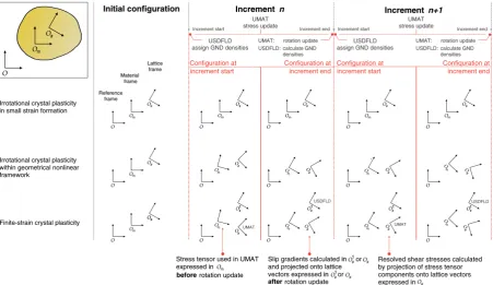
The stress-update algorithm and gradient calculation scripts are not simultaneously active in the current implementation of the crystal plasticity finite element method. The USDFLD subroutine is called twice each increment of the Abaqus solver, performing different tasks at the start and the end of the increment. This is schematically outlined in Table2.1.
Gradients of plastic slip are only computed at the end of the increment, after the stress-update algorithm has converged. GND densities are calculated accordingly. At the start of the next increment, the pre-viously computed GND densities are assigned to the material’s state variables. Using these values, the stress update algorithm programmed in the UMAT subroutine is able to calculate the GND-induced hardening terms. A small unbalance is thus introduced within each increment to be corrected in the subsequent one [10]. The assignment of the neighbouring points used for the gradient computations for each central Gauss point, is performed only at the start of the first increment for computational efficiency.
Table 2.1:Implementation of gradient computations and stress-update algorithm within global FEM-increments
Increment 1:
USDFLD: for all integration points, determine set of neighbouring points to be used in gradient calculations UMAT: perform global stress update iterations
perform lattice rotation update
USDFLD: compute slip gradients∇γ(α)and GND-densitiesρGND
. . .
Incrementn:
USDFLD: assign GND-densitiesρGNDto state variables
UMAT: perform global stress update algorithms using updated state variables perform lattice rotation update
USDFLD: compute slip gradients∇γ(α)and GND-densitiesρ GND
Incrementn+ 1:
USDFLD: assign GND-densitiesρGNDto state variables
UMAT: perform global stress update algorithms using updated state variables perform lattice rotation update
USDFLD: compute slip gradients∇γ(α)and GND-densitiesρGND
. . .
Incremental calculation sequence
The implementation in Table 2.1features the implicit, rate-independent finite-strain stress update al-gorithm from Section 2.4.2. In absence of the gradient computation script, it can thus be used to de-scribe arbitrarily large deformations. It is important to note that up to this point, the gradient-enhanced crystal plasticity formulation is not applicable in finite-strain problems. The formulation of the Burgers tensor in (2.21) limits the validity of the GND-computations in Section 2.4.3 to applications involving small-deformations. The perquisites for the finite-strain application of the gradient-enhanced crystal plasticity model will be discussed in Section3.3.
This chapter provides an overview of extensions and adaptations that were made to the theoretical framework of the crystal plasticity model. Building upon the algorithmic framework introduced in Sec-tion2.4.2, an alternative approach for multi-surface stress update algorithms is proposed in Section3.1. Herein a method is developed which solves the stress update for all slip systems simultaneously without elastic check and iterative active set update. The calculation algorithm for the gradients of slip described in Section2.4.3 is extended in two ways. At first, it is made suitable for use in combination with peri-odic RVEs in Section 3.2. The small strain gradient calculations that originate from Section2.3.1 are examined for applicability within a finite-strain formulation in Section3.3, to obtain a gradient-enhanced crystal plasticity model that can be used to describe arbitrary large deformations.
3.1 Stress update algorithm without elastic check and active set
de-termination
As discussed in Section 2.4.2, the original stress update algorithm only enters the Newton-Raphson loop if the flow criterium for at least one system is larger then 0. For the elastic case, this loop is omitted, the plastic slip increments are set to 0 and the elastoplastic moduli are taken as the elastic ones. This requires an additional check in the algorithm and involves a manual adaptation of the plastic parameters. Due to the method of updating the active set, the Newton-Raphson iterations may have to be performed multiple times in one load step. It is even possible that the same active set is solved for multiple times during the return mapping process. This results in a higher computational time and introduces the pos-sibility for the algorithm to get stuck in an endless loop, iterating between the same active sets. It thus becomes clear that it is desirable to develop a solution method that is capable of solving the plastic slip parameters for all possible slip systems at once and return positive slip values only for systems exceed-ing their respective flow criteria. By not assignexceed-ing plastic slip to inactive systems, the elastic check can be omitted. Solving the entire set of possible systems removes the necessity of defining an active set and its iterative update method.
In a conventional return mapping algorithm, the stress state is updated such that all flow criteria equal 0 in case of plastic flow. If one would omit the elastic check and employ the same algorithm for a stress state in the elastic domain, it will extrapolate an admissible elastic stress to the yield surface. This implies the condition φ = 0for both elastic as well as plastic deformation, instead ofφ < 0 for elastic andφ= 0for plastic deformation. A possibility to circumvent this problem is by introducing a modified expression for the flow criteria such that
˜
φ(α)= max0, φ(α) (3.1)
(3.1) thus replaces the elastic check described in Section2.4.2and automatically defines the active set. However, the max() function is not continuously differentiable. This is an undesirable property in the definitions of the Jacobian in the Newton-Raphson scheme and the elastoplastic moduli, where derivat-ives of the modified flow criteria with respect toφ(α)are required. A suitable, continuously differentiable approximation for themax()function will thus have to be found for the development of the new algorithm. This aspect will be discussed in detail in AppendixB. Its implementation in the algorithm described in Section2.4.2and the required modifications will be considered in Section3.1.1.
3.1.1 Implementation of modified flow criteria in stress update algorithm
With the continuously differentiable function that approximates (3.1) chosen to beφ¯=φ 2
1 + tanhφq, the Newton-Raphson scheme for updating the plastic parameters can be defined. The calculation steps that were outlined in Section 2.4.2 will be retained. Where needed, the algorithmic expressions are adapted. As a starting point, the approximated consistency conditions are redefined as
˜ r(α)=1
2˜r (α)
0 1 + tanh ˜ r0(α)
q
!!
(3.2)
wherer˜(0α)is similar to (2.30), but now obtained by taking the sum over all possible slip systems:
˜
r0(α)=σ∗:P(α)−
n
X
β=1
∆γk(β+1)P(α):Ce:P(β)−τc,k(α)(ρ) = 0 (3.3)
The linearised equation that is iteratively solved for is still of the form
r(α)−B(αβ)∗∆γ(nβ+1) = 0 (3.4)
but now the contribution of the approximation function (3.2) has to be taken into account in the Jacobian matrix:
B(αβ)∗≡ −∂r
(α) ∂γk(β+1)
=−∂r
(α) ∂r(0α)
∂r(0α) ∂γk(β+1)
=∂r (α) ∂r(0α)
B0(αβ)∗
= 1
2 1 + tanh ˜ r(0α)
q
!
+q−1cosh−2 r˜ (α) 0
q
!!
B0(αβ)∗=A(α)B0(αβ)∗ (3.5)
in terms of the original JacobianB0(αβ)as defined in (2.32) and the scalar factorA(α). In case the inver-sion of the Jacobian-matrix is a problem, the perturbation of (2.35) is performed onB(αβ)∗.
The plastic slip parameters now follow again from∆γk(α+1) = B(αβ)∗−1
r(β). It is however possible that the calculated plastic slip on some of the slip systems in not admissible in the senser(α)∆γ(α)<0. For these systems, the residualr(α)and the corresponding rows and columns inB(αβ)are set to zero and ∆γk(α+1) is calculated using this updated set of equations. This update is based on the system dropping update discussed in Section 2.4.2, with the difference that it is performed within a Newton-Raphson iteration instead of after completing all iterations. The incremental plastic slip on the originally violated systems will be set to 0 by this correction.
The updated plastic slipsγk(α+1) =γk(α)+ ∆γk(α+1) are used to calculate the updated plastic strains, stress state and flow criterion values as described in Section 2.4.2. The updated flow criterion values are checked against (2.39) to determine the convergence of the Newton-Raphson loop.
In case the solution has converged, the consistent elastoplastic moduli are calculated. In its original formulation, the expression for the elastoplastic moduli is based on the inverted JacobianB0(αβ)∗−1 that was obtained in the Newton-Raphson calculations. In the modified algorithm, this Jacobian is not directly available as it is replaced by the formulation A(α)B(0αβ)∗ in (3.5). Therefore, the original Jacobian is obtained by applying the manipulation
B(αβ)∗−1 =A(α)B0(αβ)∗
−1
=A(α)−1B(αβ)∗
−1
0 ⇒B
(αβ)∗−1
0 =A
(α)B(αβ)∗−1
(3.6) from which (2.41) can be rewritten as
Cep=Ce− n X α=1 n X β=1
A(α)B(αβ)∗−1Ce:P(α)⊗P(β):Ce (3.7)
A note on computational efficiency
Using the modified algorithmic expressions described above, the plastic slip parameters are solved for all possible systems at once. This however does not mean that information of all systems is required at all times. When calculating the incremental plastic slips using (3.4), the entire system
B∗∆γn+1=r (3.8)
is solved. The residual vectorrmay however contain many zero-entries due to the definition of (3.2). As a result, corresponding incremental slips will also remain zero. The solution procedure can be speeded up significantly by exploiting the sparsity of r. Following the calculation of the current residualsr˜(α), only the rows and columns ofB∗corresponding to non-zero entries inrare calculated.∆γis initialised as then×1-zero vector. The entries that should be assigned a plastic slip are updated by solving the reduced system
B(αβ)∗∆γn(β+1) =r(α) (3.9)
with
α∈(1, ..., n)|r(α)>0 and
β ∈(1, ..., n)|r(β)>0 . This reduces the number of calculation steps required in the definition of the Jacobian matrix and the computational time for solving the system of equations. As setting the residual of the violated systems to 0 represents a further reduction of the set of equations, the aforementioned method is still applicable with the system dropping update for in-admissible plastic slips. It should be noted that (3.9) does not fix the active set. The current active set is redefined after every update ofrand thus during each iteration.
The reduced Jacobian matrix can also be used in calculating the elastoplastic moduli in (3.7) by only summing over system indices with positive flow criteria values. This further reduces the computational time as only contribution of currently active systems are taken into account.
The flow charts for both versions of the algorithm are shown in TablesC.1andC.2for comparison of the calculation steps in AppendixC.
3.1.2 Comparison of the algorithms
To compare the functioning of both versions of the algorithm, it will be tested on various levels. At first, simulations are performed on material point level, i.e. one single (integration) point at which stresses and strains are calculated following a prescribed loading. After these initial tests, the stress-update algorithms are implemented in the FEM-software Abaqus by means of a user material (UMAT) routine. Within this section, the outcomes of the various tests will be summarised in order to compare both codes in terms of efficiency and stability.
Simulations on material point level
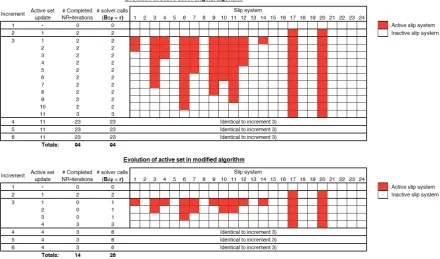
Simulations at the material point level are performed using a dedicated driver script, which can take as input a prescribed stress or strain state or a predefined deformation gradient. It is also possible to set a combined loading option. Here, certain strain components are specified and the stresses in undeformed directions are kept zero. The script thus mimics the iterative solution procedure performed by a FEM-solver per integration point. The stability of the algorithms is best tested by using a prescribed stress state or the combined loading option. As the stress-update algorithms are strain driven, these load types generally require multiple iterations to find the deformation state that matches the prescribed loading. The loading condition and material parameters used for testing are given in Table 3.1(simulation 1). The evolution of the active set for the single load step simulation is graphically depicted in Figure3.1. In both codes, the first increment is elastic and no systems are active. In the second load step, systems 17 and 20 become active. In the subsequent increments, the initially active set is larger, but reduces to
A = [17,20]after several system dropping updates. The original code performs these updates slower
Figure 3.1:Comparison of the active set evolution using both versions of the stress-update algorithm
Table 3.1:Material parameters used in the material point simulations
Material parameters for simulations 1 and 2 Prescribed stress state for simulation 1
Young’s modulus E= 210000 [MPa] σ= [420, 50, 0, -300, 0, 0] MPa
Poisson’s ratio ν= 0.3 [-]
Taylor factor c= 0.3 [-] Prescribed strains for simulation 2
Burgers vector b= 2.86·10−7 [mm] Load step Prescribed strain increments
Initial SSD density ρ0
SSD= 106 [mm
−2] 1 ∆
13= 0.025
Saturation SSD density ρ∞
SSD= 5·108 [mm−2] 2 ∆33= 0.05
Saturation plastic strain γ∞= 0.5 [-] 3 ∆
11= 0.05
Hardening parameters Q0−5: 2, 3 x 10, 8, 15 [-] 4 ∆33=−0.05
Lattice rotations φ1,Φ, φ2: 0, 0, 0 [rad] 5 ∆13=−0.05
6 ∆13= 0.01,∆23= 0.01
than the modified algorithm, as a fully converged Newton-Raphson loop is required before the update takes place and only one system is dropped at a time. In the modified algorithm, updates are performed during the Newton-Raphson iterations and all violated systems wherer(α)∆γ(α) < 0 are taken out at once. Consequently, the number of solver calls and Newton-Raphson iterations is smaller. Over ten simulation runs, the modified code on average is 32% faster.
The ability of the modified algorithm to adept to changes in the active set is tested by subsequently subjecting a material point to different states of shear and tensile deformation. Stresses in the unde-formed directions are kept zero. Details about the loading conditions and material model are given in Table 3.1(simulation 2). Averaged over five simulations, the original code completes calculation in 7.136 s, whereas the modified algorithm uses 7.175 s. The numerical results of both codes are identical up to the precision of the convergence tolerance, 10−8. Both codes can thus capture the changes in active set.
Based on the performed material point simulations, the functioning of the modified stress-update al-gorithm is comparable to that of the original code. In determining an active set by system dropping updates, it even performs faster. To gain further insight in its applicability, FEM-simulations will be per-formed using the modified algorithm and comparing it to results obtained with the original stress-update formulation.
Table 3.2:FEM-results for testing the implementation of the modified stress-update algorithm
Algorithm Lattice rotation angles Max. stress [MPa] # increments # iterations CPU time [s]
φ1 Φ φ2
Original 0 0 0 179.7 105 106 134.69
Modified 0 0 0 179.7 105 106 198.91
Original 0.3 0.2 0.5 336.0 105 116 140.74
Modified 0.3 0.2 0.5 335.3 107 123 212.16
Original 0 0.5 0.2 194.0 105 106 138.97
Modified 0 0.5 0.2 192.0 541 1804 22559.8
Simulations on FEM level
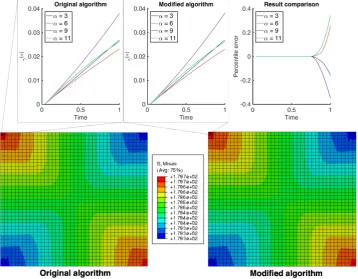
To test the functioning of the modified stress-update code in solving finite element models, it is imple-mented as user material model in Abaqus. A 100 x 100 mm square shell is meshed with 2.5 x 2.5 mm plane stress quadratic quadrilateral elements. The part is subjected to a 5 % uniaxial strain. Material parameters are identical to Table3.1except for the lattice rotations and the Young’s modulus, which is set to78GPa. Three simulations are performed, each with lattice rotation angles as defined in Table3.2. For each simulation, the Von Mises stress distribution is compared between both versions of the al-gorithm. For the top left element, results are extracted for integration point 1 to be able to compare the evolution of the plastic slips. Results of the simulations are provided in Figures3.2to3.4and Table3.2. It is clearly seen that for an increasing amount of lattice rotation, which is for observed most severely in Figure 3.4, the results of both algorithms start to differ. Also, the calculation time for the modified algorithm increases significantly.
To investigate the cause of this problem, the strain state of the first integration point of the top left element was input in the material point driver and the development of the active set was tracked. It was observed that the active set and the components of the elastoplastic stiffness tensor fluctuated severely. This behaviour was found to be caused by the update of the active set in case of negative plastic slips, as defined under item 4(b) of Table C.2. Previously active and admissible sets can be rendered inactive by this update at once, leading to severe changes in the active set and premature convergence of the Newton-Raphson iterations. It must be noted that the original algorithm suffers from the same convergence issues if the active set prediction is turned off. In general, the modified algorithm converges and yields the same results as the original code if this version can converge without active set prediction.
3.2 Gradient calculations in periodic models
Periodic boundary conditions are often applied to Representative Volume Elements (RVEs) used in crystal plasticity simulations. These are rectangular (2d) or box shaped (3d) FE representation of a polycrystalline material and consist out of a limited amount of grains. These grains may be cut by the boundaries of the RVE. Cut-off parts are continued at the opposed edge of the RVE. For a more elabor-ate discussion of these topics, the reader is referred to Section5.1.
Recalling the gradient calculation procedure outlined in Section 2.4.3, gradients are calculated from neighbouring integration points within the same grain. A neighbouring point is taken into account in the calculations if its distance to the central integration point is less than a predefined search radius. However, if a cut grain is continued at the opposite side of the model, integration points from that region may never lie within the search radius and will thus not be included in the calculations. This causes gradients near the RVE-boundaries to be essentially based upon one-sided difference schemes instead of a more accurate two-sided scheme. Therefore, an extension to the gradient script for application to two-dimensional periodic RVEs has been developed.
Figure 3.2:Comparison of the FEM-results obtained using both stress-update algorithms. Plastic slip evolution is displayed for integration point 1 of the top left element. Lattice rotation angles0, 0, 0radians
Figure 3.3:Comparison of the FEM-results obtained using both stress-update algorithms. Plastic slip evolution is displayed for integration point 1 of the top left element. Lattice rotation angles0.2, 0.3,0.5radians
[image:24.595.119.478.427.710.2]Figure 3.4:Comparison of the FEM-results obtained using both stress-update algorithms. Plastic slip evolution is displayed for integration point 1 of the top left element. Lattice rotation angles0, 0.5, 0.2radians
Within the original RVE, a fictitious inner rectangle is drawn at an offset to the outer shape with the size of the search radiuss. The area between the two rectangles is divided into eight search regions, as shown in Figure3.5a. Additionally, a number of eight tiles is identified as indicated in Figure3.5b. Integration points that lie within the eight search regions will be mapped to the tiles by coordinate transformations. For instance, a point within region 1 is mapped to tile 6 by the shifting vector{W,0}T. A point in region 4 is mapped to tiles 8, 1 and 2 using the transformations{0, H}T,{−W, H}T and{−W,0}T, respectively. This mapping is handled in the initialisation step of the gradient script in the first FE-increment as in Table3.4.
The gradient calculation step is essentially left unaltered. The only difference with respect to the original formulation is that for shifted integration points, the distance to the central integration point is calculated from the shifted coordinates, whereas the slip data is extracted from the corresponding integration point in the original RVE. This is outlined in Table3.3.
[image:25.595.126.472.101.375.2](a)Search regions within the RVE (b)Virtual tiles
Figure 3.5:Search regions and tiles required for periodic gradient calculations
3.2.1 Comparison of the gradient codes
Figure 3.6:Comparison between GND density distribution calculated with and without periodic slip gradients
Figure3.6shows the total GND density as calculated by the gradient script using both the non-periodic as well as the periodic implementation. The intensity plot on the right indicates the difference between both colour plots. The higher the colour intensity of this plot, the greater the difference in GND density. The RVE depicted here consists of 29 grains with different orientations and a FCC-lattice. It is subjected to uniaxial tension in horizontal direction. As it serves the sole purpose of providing a qualitative com-parison between the methods, further details about the model are omitted.
The majority of the distribution is the same in both colour plots, as expected from the fact that only points near the outside of the RVE are affected by the modified calculations. The greatest differences are indeed observed in this outer region, as indicated by the intensity plot. The small islands of negative GND densities, indicated in dark blue and visible near the RVE edges in the left plot, are removed by adding the periodic calculations. As a result, no colour differences between opposed edges are found anymore. The GND distribution is thus fully periodic now. The differences that are found in the interior grains are caused by slight changes of the response to the macroscopic loading caused by differences in hardening in the exterior grains.
Table 3.3:Modified calculation step for periodic gradient computations.Modifications shown inblue
For each original integration pointj
Loop over integration pointskthat were identified to lie within search radius of pointj:
Ifkis a shifted integration point:
1. Get number of original integration pointkicorresponding to the shifted co-ordinate
2. Calculate gradient of slip based on distance between pointsjandkand slip values at pointsjandki
Else:
Calculate gradient of slip based on distance between pointsjandkand slip values at pointsjandk
Pseudo-code for calculation step
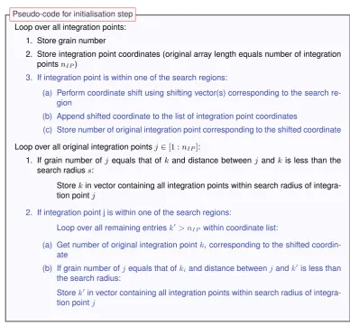
Table 3.4:Modified initialisation step for periodic gradient computations.Modifications shown inblue
Loop over all integration points: 1. Store grain number
2. Store integration point coordinates (original array length equals number of integration pointsnIP)
3. If integration point is within one of the search regions:
(a) Perform coordinate shift using shifting vector(s) corresponding to the search re-gion
(b) Append shifted coordinate to the list of integration point coordinates
(c) Store number of original integration point corresponding to the shifted coordinate Loop over all original integration pointsj∈[1 :nIP]:
1. If grain number ofjequals that ofk and distance betweenj andkis less than the search radiuss:
Storekin vector containing all integration points within search radius of integra-tion pointj
2. If integration point j is within one of the search regions:
Loop over all remaining entriesk0> nIP within coordinate list:
(a) Get number of original integration pointkicorresponding to the shifted coordin-ate
(b) If grain number ofjequals that ofkiand distance betweenjandk0is less than the search radius:
Storek0in vector containing all integration points within search radius of integra-tion pointj
Pseudo-code for initialisation step
3.3 Determining GND-densities in a finite-strain formulation
In a general finite strain framework, especially when large rotations are present, the simplifications mentioned in Section2.3.1are no longer valid. This may affect the calculation procedure of the GND-densities. Within this section, the theoretical framework of GND-density evolution in a finite-strain frame-work will be examined. Comparison of these results with the formulations in Section2.3.1will provide insight into the extent to which these formulations can be applied when simulations are to be performed that exceed the assumption of small deformations.
Within the finite strain setting, proper attention must be paid to the relations between plastic slips dis-tributions and slip system orientations between the different configurations shown in Figure 2.1. As introduced before, the finite-deformation crystal plasticity framework is given by the multiplicative de-composition of the total deformation gradient as
F=FeFp (3.10)
to describe the mapping from the reference space B0 to the observed space Bvia the intermediate configurationB¯, representing the lattice space [31]. If a unit normal vector in the reference configuration is denoted asn0and its counterpartnis given in the final configuration, the unit lattice normal is defined in terms of the elastic and plastic deformation gradients as
n#=
F−pTn0
|F−pTn0|
= F
T en
|FTen| (3.11)