Brazilian foreign trade : fixed and time varying parameter models

University of Warwick institutional repository: http://go.warwick.ac.uk/wrap

A Thesis Submitted for the Degree of PhD at the University of Warwick

http://go.warwick.ac.uk/wrap/53070

This thesis is made available online and is protected by original copyright. Please scroll down to view the document itself.

FIXED

AND

TIME

VARYING

PARAMETER

MODELS

by

Marcelo S. Portugal

Thesis _submitted in _partial fulfilment

of the requirements for the degree _of

Doctor _of Philosophy

University _of Warwick

Department _of Economics

Table _{of Contents}

... i

Acknowledgments ... v

Summary ... vii

Chapter I- Introduction ... 1

Chapter II _{- Modelling} Trade Equations ... 8

I) Introduction ... 8

II) The Specification _of Trade Equations... 9

1) The Production Theory Approach ... 9

2) The Perfect _{and Imperfect} Substitutes Models... 12

3) Other _{variables of} Interest _... 19

3.1) Import Equations _... 19

3.2) Export Equations ... 22

4) Some Econometric Considerations ... 25

4.1) Functional Form _... 26

4.2) Dynamics _{and Stationarity ...} 26

4.3) Simultaneity _... 28

4.4) Aggregation _... 29

4.5) Parameter Stability _... 30

III) Brazilian Trade Equations _... 32

1) Import Demand Equations _... 33

2) Export Equations _... 40

IV) Conclusions _... 44

Chapter III _{- Brazilian} Trade Policy, 1947-1988... 46

I) Introduction _... 46

III) The Multiple Exchange Rate Regime, 1953/57... 50 IV) Tariff Reform _and Exchange Rate Unification,

1957/64

... 53 V) The "Crawling Peg" System _and Incentives to

Exports, 1964/74

... 57 VI) The Oil _{and Debt} Crises, 1974/83

... 62 VII) The Relaxation _of Controls, 1984/88... 69 VIII) Conclusions

... 73 Appendix III. _{1 - Main-Economic} Indicators... 75

Chapter _{IV - Time Varying} Parameter Models, Unit

Roots _{and Cointegration ...} 84 I) Introduction

... 84 II) Different Models Proposed

... 86

1) Purely Random Model

... 86

2) The Adaptive Regression Model

... 88

3) Systematic Parameter Variation _... 93

4) Switching Regressions

... 96

5) Some Ralations Between _{the Models ...} 101

III) The Kalman Filter _... 103 1) Finding the Prediction Equations

... 106 2) Finding the Updating Equations

... 107 3) The Recursive Estimation

... 111 4) The Stochastically Convergent Coefficient

Model

... 113 5) The Bayesian Approach

... 114 5.1) A Bayesian Interpretation _of the

Prediction _{and Updating} Equations _... 114

5.2) Variance Learning and Discount Factors... 117

6) Autoregressive Residuals

7) Recursive Least Squares

... 120 8) ARIMA Models in State Space Form _... 121 9) Unobserved Components Models

... 123 10) Smoothing

... 125 IV) Trending Variables, Unit Roots _and

Cointegration

... 126 1) The Engle-Granger Procedure

... 127 2) The Johansen Procedure

... 130 3) Seasonal Cointegration

... 134 4) Encompassing

... 139

IV) Conclusions _... 144

Chapter V- Estimations _of Import Demand Equations.... 146

I) Introduction

... 146

II) Fixed Parameter _{Models ...:... 147}

II. 1) Quarterly Data Estimations

... 149 1) Import Demand for Intermediate Goods... 150 2) Import Demand for Capital Goods

... 153 3) Total Import Demand

... 159

11.2) Annual Data Estimations

... 162

1) Different Measures _{of Capacity} Utilization... 163

1.1) Measures _{with a Fixed} Potential Output

Growth Rate

... 165

1.2) Measures _{with a Varying} Potential

Output Growth Rate

... 167 1.3) Comparing the Different Measures _... 173 2) Import Demand for Intermediate Goods

... 177 3) Import Demand for Capital Goods _... 182 4) Total Import Demand

... 185

III. 1) Annual Data Estimations

... 188 1) Total Import Demand

... 189 2) Import Demand for Intermediate Goods

... 199 3) Import Demand for Capital Goods

... 204 111.2) Quarterly Data Estimations

... 209 1) Total Import Demand

... 210 2) Import Demand for Intermediate Goods _... 216 3) Import Demand for Capital Goods

... 220 IV) Conclusions _{and Remarks}

... 224 Appendix _{V. 1 - The Johansen} Procedure

... 227 Appendix _{V. 2 - Data Appendix}

... 232

Chapter _{VI - Estimations of} Export Equations

... 240

I) Introduction

... 240

II) Fixed Parameter Models

... 241

II. 1) Annual Data Estimations

... 242 1) Total Non-Coffee Exports

... 243 2) Industrial Exports

... 248

11.2) Quarterly Data Estimations _... 251

1) Total Non-Coffee Exports

... 252

2) Industrial Exports _... 257

III) Time Varying Parameter Models

... 259

1) Kalman Filter Estimations _... 260

2) The Switching Regressions _{Approach ...} 264

3) The Bayesian Approach

... 270

IV) Conclusions _and Remarks

... 283 Appendix _{VI. 1 - Data Appendix}

... 286 Chapter VII _{- Conclusions}

... 292 References

ACKNOWLEDGEMENTS

I _would like to _{express my gratitude to several}

people, all of whom directly and indirectly _contributed

to the _{successful completion of} this thesis. First _{of all}

I _would like to thank _{my supervisor,} Professor Ken

Wallis, for his _{advice and encouragement over the last}

three _years. Our _{weekly meetings} helped to keep _{me on}

track _{and contributed substantially not only} for the

completion of this thesis but also to my understanding of

econometrics. I would also like to thank Dr. David Collie

for his _{comments, especially regarding the trade models}

discussed _{in chapter} two. _{I am indebted} to Professor Jeff

Harrison for his help _with the Bayesian _estimations in

chapter six. I am most grateful to Sanjay Yadav _{not only}

for his _{comments on all parts of} this thesis but, _also

for his friendship _and for the best Indian food I have

ever tasted. Giovanni Amisano helped _{me to understand} the

Johansen _{procedure and} to _{obtain and use a program} to

compute this procedure and the Phillips and Perron test.

Finally, I _would like _also to thank Professor Alan

Winters _and Mr. Dennis Leech for helpful _{comments and}

discussions.

To Miriam I have _{an eternal} debt _{of gratitude} for

her love, _{encouragement and understanding} over the last

seven years. My son Daniel, who was born in England while

I was writing this thesis, helped _{substantially} to _speed

always awake before _{seven o'clock.} My family in _Brazil

also have my gratitude for their _{moral support and help}

in sorting out hundreds of bureaucratic problems.

Finally, _{I would} like to _{gratefully acknowledged the}

financial _support from CAPES the Brazilian federal _agency

SUMMARY

In this thesis _{we estimate and analyse several}

econometric models for the Brazilian trade _equations. A

major attention is given to the _{questions of stationarity}

and parameter instability. We test for the _{presence of}

unit roots by using the Dickey _{and Fuller, and Phillips}

and Perron tests and the Johansen procedure, and apply a

error correction mechanism to the data. To investigate

the _{question of parameter} instability _{we use the Kalman}

filter in both _{classical and bayesian approaches and the}

switching regressions technique. These tests _and

estimations are performed using both annual and quarterly

disaggregated data. _{We show} that, in _{some cases,} the

trade _{equation coefficients are} indeed time _varying. The

changes in the trade elasticities are then related to

changes in the trade _{policy regime and to} the industrial

CHAPTER I

INTRODUCTION

For the last ten _years foreign trade has been _a major concern of Brazilian _{economic policy. The} debt crisis in 1982 brought about the need to _{obtain a large} trade _surplus to _offset the _{current account} deficit. As foreign loans _suddenly became _unavailable, the _{only way} to keep _paying interest _{on the foreign debt and ensure} the flow _of imports _was through _{a massive} increase in exports.

These _severe balance _{of payment problems motivated}

several attempts to _estimate trade _equations for _policy

analysis. However all this empirical work shares the

assumptions of stationarity and constant parameters. The

main concern of this thesis is that these assumptions may

not be appropriate in this context and, therefore, we

propose to investigate this matter by using new

techniques that deal _{with non-stationary series and time}

varying coefficients.

As far _{as the question of stability} of the Brazilian

trade _{equations coefficients} is _concerned the _existing

literature is _quite inadequate. In most cases this

question is mentioned but the treatment does not go

further than applying structural stability tests.

Regardless _of the _{result of the structural} stability test

relationship can either be gradual or sudden, and in either case the _{resulting parameters will be biased and} inconsistent if _allowance is _{not made for the shifts.} There _are in fact _{good reasons} for _{expecting that trade} relationships are subject to both types _{of changes.} Gradual _changes in the _{elasticities can come about as the} pattern of trade changes during the _{process of economic} development _{or as} the _{result of changes} in _government trade _policies. Sudden _{shocks such as changes} in the exchange rate or exchange rate regime, or large oil price

increases _{can also fundamentally alter the basic demand} and supply relationships". ' In _{a more general} framework Lucas (1976) has _{also claimed} that _{since agents} have rational expectations the parameters in the _econometric relationships may not remain constant after changes in the _{policy regime.} Additionally, _parameter instability

may also be expected as a result of Orcutt's "quantum effect" or from aggregation problems. 2

Given the large _changes in the _{structure of}

Brazilian trade _{and sharp modifications} in trade _policy

during the last three decades, the Brazilian trade

equations might be particularly subject to parameter

instability.

Brazilian _{exports previously} relied on coffee but

are now based on manufactured and semi-manufactured

goods. The import _{substitution process has}

completely

reshaped the industrial _{structure. Two}

major import substitution plans, the Piano de Metas _and the II PND,

were particularly important in _{encouraging import}

substitution in new industries, _especially in the

intermediate _{and capital goods sectors. Moreover, this} import _{substitution process also contributed to alter the} composition of imports, substantially reducing the _share

of consumer goods. _-

Exchange _{rate policy} has _changed from _{a single to a}

multiple rate system and back again. Direct import

controls and additional costs have been imposed on

imports from time to time. Substantial _changes in tariff

policy have also taken place and a quite generous system

of export incentives has been introduced.

The main objective of this thesis is the estimation

and analysis of time varying parameter models for

Brazilian foreign trade. These _{estimations are performed}

mainly by using the Kalman filter in both _{classical and}

Bayesian frameworks. We then try to _associate the _changes

in the _{coefficients with changes} in the _{policy regime or}

the import _{substitution process.} The thesis _{also provides}

a case study of the relative advantages and disadvantages

of some of the different statistical methods that have

been proposed.

The assumption of weak stationarity, that is, that

the first _{and second moments of a time series} are

time-invariant, _{played an} important _part in the

Subsequently _{time series analysts drew attention to kinds} of trends, in _{mean and variance, and Box and Jenkins}

(1970) _{popularized the approach of differencing}

a series to _reduce it _{to stationarity. Such a series is}

referred

as difference-stationary _or integrated _series,

equivalently we can say that its autoregressive operator

contains one or more unit roots. Box _and Jenkins

presented a number of judgemental methods for determining the _required degree _of differencing, _that is, _{the order} of integration or number of unit roots. It was only later that formal hypothesis tests _were developed. 3 Although _one can make a series stationary by taking first differences,

this _approach implies loosing _all the long _{run properties} of the model.

Stationarity _{was always} taken for _granted in

previous work on Brazilian foreign trade. _{No attempt was}

made to test for the presence of unit roots in the data.

Given the _{results obtained} by Nelson and Plosser (1982),

revealing the _{presence of unit roots} in _{many economic}

time _series, it _seems inadequate to treat this question

by assumption. Actually, _{evidence of} the inadequacy _of

assuming stationarity when dealing with economic time

series had been given a long ago by Granger (1966). The

"typical _{spectral shape", with} high _{values at} low

frequencies, _observed in _economic time _series is _an

indication _of how important trends _are in this kind of

series.

Therefore, _{the approach}

adopted in this thesis

consists in first testing for the _{presence of unit roots}

using a number of test statistics available, going from

the _simple Dickey _{and Fuller test to the recent}

and

sophisticated Johansen _{procedure. Once the presence of}

unit roots is observed we test for _{cointegration and use}

a error correction approach to model the data.

The advantage of using an error correction mechanism

is that _economic theory is _{used to establish only the}

long _{run relationship} between _{the variables, while the}

short run dynamics is data determined. _{A general to}

specific approach is adopted to deal with the question of

dynamics. We _{start with a} fairly _{general dynamic}

structure and test successive restrictions that _are data

acceptable and economically meaningful to obtain a

simpler dynamics.

The _{question of} how to deal _with dynamics,

especially when using quarterly data, is _{also a common}

problem far as the empirical work on Brazilian trade

equations is concerned. None of the existing work employs

anything more complex than the simple partial adjustment

model. The use of a error correction mechanism and the

general to specific approach mentioned above is also

useful in overcoming this problem.

The thesis _{proceeds as follows. In chapter two}

we present the production theory _and the _{classical supply} and demand approaches for _{modelling trade equations. In} the _{case of} the _{production theory approach the}

question of parameter instability _{can be addressed by choosing the}

appropriate profit function. We _{use a translog}

specification as an example of a profit function that generates non-constant elasticities. Some discussion _of

usual econometric questions, such as the _{choice of}

variables and functional form, treatment _of dynamics _and stationarity and aggregation, is also included in this chapter. Finally, we present a critical survey of the

relevant empirical literature on Brazilian trade

equations.

The _{next chapter provides a general presentation of} Brazilian trade _policy for the _period 1947 to 1988. During this _period Brazil has _{experienced several abrupt}

changes in the trade _{policy regime.} There _was the

creation of the tariffs system, the change from multiple to _{single exchange rate,} the _{creation of an export}

incentive _program, two _major import _{substitution plans} and several measures to control imports. In other words, this _{chapter contains} the _policy background _necessary to analyse the changes in the trade equation coefficients.

In _chapter four _{we deal with} the econometric methods that _will be _used in the estimation work. Most of this

chapter is concerned with presenting and comparing

several different time varying parameters models. This

adaptative _{regression model, the systematic}

parameter variation model _and the _{switching regressions model.} Especial _attention is _{given to the Kalman filter and its} use in both classical and Bayesian framework. _{Some other} econometric issues regarding unit roots and cointegration

are also discussed, _namely the Johansen _{and Engle and}

Granger _{procedures, seasonal cointegration}

and encompassing.

The fifth _{and sixth chapters present and discuss}

the _{empirical results} for imports _{and exports,}

respectively. In these two _chapters the trade _models

presented in chapter two _{are estimated using the}

econometric methods discussed in chapter four and the results are analysed against the background of policy change discussed in chapter three. The _classical Kalman filter _approach, the _{switching regressions model and} the Bayesian Dynamic Linear _{model are used} to _estimate time varying trade _{elasticities. We will associate} the _changes in the _{coefficients with} the _changes in the trade _policy regime.

Finally, in _{chapter seven we present general}

conclusions of the thesis, including some policy

implications _of the _{results obtained} in _chapters five _and

CHAPTER II

MODELLING TRADE EQUATIONS

I) Introduction

In this _{chapter we will address the question of how}

to _model trade _{equations. We will discuss not only the}

theoretical _aspects but _{also some of the applied work}

using Brazilian data.

We will deal _{as well with some of the practical} econometric problems involved such as which variables to use, how to model the dynamics, _parameter instability _and stationarity.

All _{empirical work on} Brazilian trade _equations to

date have _assumed that the _{parameters are constant.} This

may be an unrealistic assumption, if price and income

elasticities in trade equations vary not only cyclically,

according to movements in the business _{cycle, but also as}

a result of the implementation _of different trade

policies or changes in the pattern of trade due to the

process of economic development. Such parameter

instability _might be _{particularly expected} in the

Brazilian _{case, given} that in the last thirty years there

have been several abrupt changes in trade policy and two

major import substitution programs.

Following this introduction, the chapter has three

sections. In the next section, we present the main

together _{with some empirical issues. The third}

section contains a discussion _of the _{empirical work available on} trade _equations in Brazil _{and the last section presents} the _{conclusions and remarks.}

II) The Specification _{of Trade Fauatigns}

There _are two different _{approaches to the modelling} of trade equations. The traditional _{approach, surveyed by} Goldstein _and Khan (1985) _{and Magee} (1975), _{adopts a} household _{model treating traded goods as final goods that} enter the _{consumer sector} directly. An _alternative approach, surveyed by Woodland (1982) _{and Kohli (1991),}

models trade equations from a production theory

framework.

1) The Production Theory AQUroach

In this _model the _{small country} hypothesis is

adopted, implying that _only import demand _{and export}

supply have to be _{estimated. All} imported _{goods are}

supposed to be intermediate _{goods, used} by the _production

sector as inputs. On the _other hand, _{exported and}

domestic _{goods are assumed} to _{be separable outputs of} the

production sector. That is, in this model there is no

consumption of traded goods, since all imports are inputs

while exported goods are different from domestic

production. Duality theory is used to derive

econometrically convenient equations.

Import _{and export decisions}

are made by profit maximizing

firms _{under perfect competition}

conditions. The firms

choose the optimum imports _{and output mix given a vector}

of domestic and international _{prices and a vector of}

domestic _primary factor _{stocks. The technology is}

represented by a production possibility _set from _which

the _profit function _can be derived. _{Therefore, given the}

production possibility set T we can define the _restricted

profit function, which has the usual _{properties, as}

lr(p, v) = maxx { px: (x, v) E T}

where x is a vector of net output (imports enter with a

negative sign), v is a vector of fixed inputs and p is a

positive vector of domestic and international prices.

Using Hotelling's _{Lemma we obtain}

x= Vp r(p, v) (1)

where V is the _vector differential _operator. Assuming

that _{capital stock} is fixed in the short run, the _system

of equations (1) represents the short run domestic output

supply and the short run export supply and import demand

functions. Similarly, _{we can obtain} the _{system of} inverse

demand for domestic _primary inputs (if the derivatives

exist)

w= Vv 7[(p, v) (2)

where w is the vector of factor prices.

To _make the _{model operational we} have just to

In(z)

_{= aoo}

+7

aio

+

a, 3

(3)

iij

Using (3) _{we can write the translog profit function asp}

In ýt =a bi _{In pi +} 1/27-7-

_Cih

iih

di _{In vj +}

1/277

e3

,jk

+77

v,

(4)

where ci j= ci i and ej k= ek j. To ensure that lt is

homogeneous _of degree _one in _{prices requires} that

bi _{=1 and fi j =7-}

_Cih

ijh

(5)

while to ensure that r is homogeneous of degree one in

domestic _primary inputs _requires that

=0. (6)

ei k

dj _{=1 and} ý _{f; j =7-}

jjk

By logarithmic differentiation _{we obtain}

aln

_?

_Fla

( a?

_{r/api ) /? r}

/? r

,

91

n

_{= v;}

_{( alr/av;}

_{) Or = v;}

/? r = si

Applying (7) to (4) _{we have}

Si = bi +7- Cih In ph +7- fij in

vj

hi

si = d3

+1

ejk

(8)

(7)

1) The choice of functional form is arbitrary. Diewert and Morrison (1989), for example, use a biquadratic

These _{equations can then be estimated}

econometrically to

obtain the _{unknown parameters. Note that,}

since _{Si and si}

add up to one, only n-1 equations _{have to be estimated}

in each system

One interesting _{feature of this}

method is that it

allows the estimation of all cross elasticities of the

domestic _supply, labour demand, import _{demand and export}

supply. Moreover, since the functional form _chosen for _it

is not a constant elasticity one, these elasticities can

be estimated for _{each point in time.}

Ei

j_

/xj

) a(air/ap+ )/api

2) The Perfect _{and Imperfect Substitutes Models}

In terms _of the traditional _{approach, as shown} by Goldstein _and Khan (1985) _{and Magee} (1975), there _are two different _{ways to model trade equations, depending on} whether domestic and foreign products are assumed to be

perfect or imperfect substitutes. In the imperfect

substitutes model, the products are supposed to be

slightly different, in such a way that prices are also different.

Thus, the demand _{and supply curves} for imported

goods can be written as a function of national income,

and prices of domestic and imported goods. What is

relevant for the importers is not only the prices, but

actually the final _{cost paid} by the product measured in a

common currency. The demand and supply of imports can

Md = f(Yn, EPm, Pd, T), (9) f> >0 f2 _{<0 f3 >0 f+ <0}

**

M$ =9( Pm , Pd , S* , Yn ), (10) 91 >0 92 <0 93 >0 g4 >0

Md = Ma 7 (11)

where Yn is nominal income, P, _{and Pd are the import and} domestic _price levels, E is the _{nominal exchange rate, S} is the _{rate of export subsidies2}

, and T stands basically for tariff, but _{should also} include _{transport costs,} insurance _{and all other factors that represent}

an additional cost for the importer. _{The asterisk is used to} differentiate between the foreign _{and home economies. The} aggregate demand function depends _{positively on nominal} income _and domestic _{prices, and negatively on} import prices measured in local _{currency and} the tariff _rate, while in the _supply function import _prices, the foreign subsidy to _exports, foreign income have the _positive sign, and foreign domestic prices a negative sign.

In the _{same way, demand and supply} for _{exports can}

be written as a function of effective prices, including

exchange rate and export subsidies, and external income.

**

Xd = 1( Px, Pd, Yn, T* ), (12) 11 <0 12 >0 13 >0 14 <0 X8 = h( EPx _, Pd

, S, Yn ), (13) hi >0 h2 <0 13 >0 h4 >0 Xd = X99 (14)

2) Note that the _supply of imports for a country is also

the _{supply of exports} from the rest of the world to the

where Px is the _{export price index. The supply}

of exports depends _{positively on export prices in terms}

of domestic

currency, export _{subsidies and domestic income,}

and

negatively on domestic _{prices, while the demand for}

exports is positively _related to foreign domestic _prices and foreign income, and negatively with export prices and tariff _rates in _{the rest of the world.}

As is _{common in the literature,}

some additional hypotheses _can be _{used to simplify the model presented} above. First, the _{estimation of supply and demand curves}

is _some times _{said not to be necessary. If one assumes} the _{supply curves to be completely elastic, only the} demand functions have to _{be estimated. Although it may be} possible for _{a country} to buy its imports in the _world market without changing the _price, the _{same does not seem}

plausible for exports. Unless there _exists idle _capacity, or, more generally, unless the _{export sector operates} subject to _{constant or} increasing _returns to _scale, it

seems unlikely that, at least in the _{short run,}

production could be expanded without an increase in

prices. In other words, although it is plausible to assume that _{a country} is _{a price} taker in the _world market, it is less plausible to assume that the rest of the _world is _{also a price} taker _{with respect} to the home economy. One explanation sometimes offered to justify the

estimation of demand equations only is that price

which "implies that _{within a range of variation in the}

data _{any quantity can be supplied at the given prices". 3}

If that is _{not the case, the import and export}

prices cannot be treated _{as exogenous variables, and a}

simultaneous model must be estimated. _{The estimation of}

the demand equation model alone, when the supply curve is

not totally elastic, would lead to an inconsistent and

downward biased _{estimate of the price elasticity of}

demand. _{The estimated price elasticity of demand would be}

a weighted average of the actual demand and supply

elasticities.

Another way of reducing the _{number of equations} to be estimated is to _adopt the "small _country" hypothesis. If the _{country's share} in _world imports _{and exports} is small, the supply of imports and the demand for exports will be completely price elastic or, at least have a

substantially high price elasticity. Thus, the import and export volumes will depend only on the demand for imports

and supply of exports functions, since the country will be able to buy its imports _{and sell} its _{exports with no} feedback _{on prices.} If that is _not the case, once again a

simultaneous model must be estimated, otherwise the

coefficients will be inconsistent and biased.

In the literature on trade equations it has been

common to _adopt the "small country" hypothesis for

imports, _{estimating only a demand equation,} while in the

case of exports the use of a simultaneous approach has

often been preferred.

A second supposition, common not only in work on

trade equations but _also in _consumer theory _{as a whole,}

is the _{absence of money illusion. This assumption implies}

that the functions _are homogeneous _of degree _zero in

prices and nominal income. One can then normalise the

variables by the domestic price level, using real income

and relative prices as explanatory variables.

Another possible simplification is to combine prices

and tariffs or subsidies into a single variable.

Sometimes it is _argued that tariff _and import _prices have

different _{effect on} imports. This _{could result} from

importers _{regarding changes} in tariff as permanent, while changes in import prices are regarded as temporary, or

from the fact that changes in tariff are usually

announced in advance. 4 The same line of argument applies to _{export subsidies.} In the case of tariffs, empirical work has shown that import prices and tariffs have equal effect on import demand. 5

The previous model can then be rewritten as

Md = f( Y, EPm (1+T)/ Pd ),

<0 f> >0 f2

*

Ms = g(Y* , Pm ( 1+T)/ Pd ), gi >0 g2 >0

* Xd =1( Y*

, Px ( 1+T* )/ Pd ), 11 >0 12 <0

XS = h( Y, EPx ( 1+S)/ Pd)- hi >0 h2 <0

(15)

(16)

(17)

(18)

Until _{now we have dealt}

with equilibrium _{models. The}

disequilibrium _{models applied to trade}

equations that _are

available in the literature _{are generally}

of a very

simple fashion. It is _{normally assumed that the}

optimum

and actual levels _of imports _{or exports are different. A}

partial adjustment _model is then _{proposed to model the}

disequilibrium. 6

More _{recently, other kinds of disequilibrium}

models have been _{proposed. These models follow the}

work of Fair and Jaffee (1972), Fair _and Kelejian (1974) _{and Maddala} (1986). The idea is to divide the _sample into _{points on}

the demand _{and supply curves. Although the maximum}

likelihood _{approach to the sample separation problem is} more efficient, simple methods using the _{price variation} are often used. Rios (1986) _{and Fachada (1990), for} example, have used the methods proposed by Fair _and Jaffee (1972) _{to estimate a disequilibrium model for the} Brazilian _exports.

On the other hand, if domestic _{and foreign goods are}

assumed to _{be perfect substitutes,} having _{a common price}

given by world supply and demand, price differentials

will play no role in determining the _{volume of} trade. In

this _case, imports _{and exports could be modelled as the}

difference between domestic _{demand and supply.}

Let _{D and S be the} total domestic _{demand and supply}

of the traded good, Pd is the domestic _price, Y is real

income _{and F is some cost variable.? Then}

the _perfect

substitutes model _{can be written as}

D= f(Pd, Y) (19)

f1 <0 f2 _>0

S= _{g(Pd , F)} (20)

91 >0 92 <0

M= D(Pd _{, Y) - S(Pd , F)} (21) X= S(Pd, _{F) - D(Pd,} Y)- (22)

One _{should note} that in this _case there _{are no} explicit demand for imports or supply for _exports. The model describes only excess demand, and excess supply of domestic _{goods, assumed to} be _satisfied by imports _and exports. The country's ability to influence world prices will depend basically on its share of the world market and on its own price elasticity of supply and demand.

The _{choice of} the _{perfect or} imperfect _substitute model will depend essentially on the kind of product or

the level _{of aggregation we are considering.} For

manufactured goods or aggregates such as consumer and

capital goods, the imperfect substitute model seems

adequate, while for homogeneous goods such as crude oil, wheat or coffee the perfect substitute model is more appropriate. 8

7) In this case, as Enoch (1978) shows, a possible

measure of competitiveness is relative costs instead of

relative prices.

3) Other Variables _{of In erest}

3.1) Import Equations

It is _{common place in the}

empirical literature _on

import demand to include _{some other variables to}

account

for _{non price restrictions, differences between}

the

cyclical and secular income _{elasticities, and for}

long _{run trends in the volume of imports. 9}

In the _{case of non price restrictions, the basic} argument is that there _{are extra costs that are not} normally reflected in movements of prices. Depending _on which phase of the business cycle the _economy is in, delivery lags _{can change considerably, leading to an} increase _{or decrease in imports. To deal with this} problem, it is common to introduce a capacity variable such _{as Y/YP , where} Y and YP are respectively actual and potential output. Thus, _when the _economy is _overheated,

imports _{tend to increase, whereas in a phase of}

widespread spare capacity the volume of imports should decrease.

Another _{point, raised} by Khan _and Ross (1975), is that _{one should} distinguish between _{cyclical and secular} effects on the demand for imports. They claim basically

that _{one should use not only actual} income _{as an}

explanatory variable, but also its potential value. Their

model is a kind of partial adjustment model, where

current imports depend _{on current income}

and the "potential demand for imports" _or, in _{other words, the} long _run demand for imports, _{depend on the potential} income. Then, by _{using a partial adjustment hypothesis,} where deviations between the _{actual and potential demand}

for imports _{are a fraction of the deviation between} actual and potential income, _{they end up with an equation}

in terms _{of price, actual real} income _{and its potential} value. In analytical terms

1n Md = ao + al in Pt _{+ a2 ln yt + ut (23)} In Mpd = bo + bi In Pt + b2 In YP + vt (24)

t

and

In Md - in Mpd =d( 1n yt - 1n yP )+ _{wt .} (25) ttt

Substituting (24) into (25) _{we get} the _estimating equation

In Md = bo + bi In Pt +d In yt + (b2-d) In yP + et (26)

tt

where et= vt + wt. Note that the sign of the coefficient

of potential income can be either positive or negative,

depending _{on the relative sizes of b2 and d. Intuitively,}

one can think of this _sign being _{positive or negative,}

depending _on the _{gradual changes} in the demand for

imports _{over time. If structural changes lead to a more}

open economy, with an increased proportion of imports in

relation to income, this _coefficient should be positive,

and vice versa.

Finally, _{a third variable normally} found in import

equations is the time trend. The inclusion of this

accounting for long _{run changes in the economy}

and consequentially in the _{structure of} imports10. _{Again, the} sign of its coefficient could be either positive or negative, depending on how successful is the import substitution process. A time trend has _also been _{used as} an explanatory variable in the _models that _adopt the production theory approach. Kohli (1978), for _example, uses a time trend to account for structural changes in both import demand _{and export supply} functions.

One _{should note} that _although these _{variables may} improve the fit _of the _equation, in theoretical terms there is _{not much} that _can be said, since in all cases the _{expected sign of} the _coefficients is _{not clear.} Even

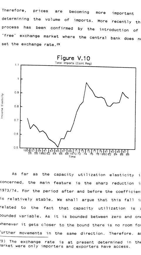
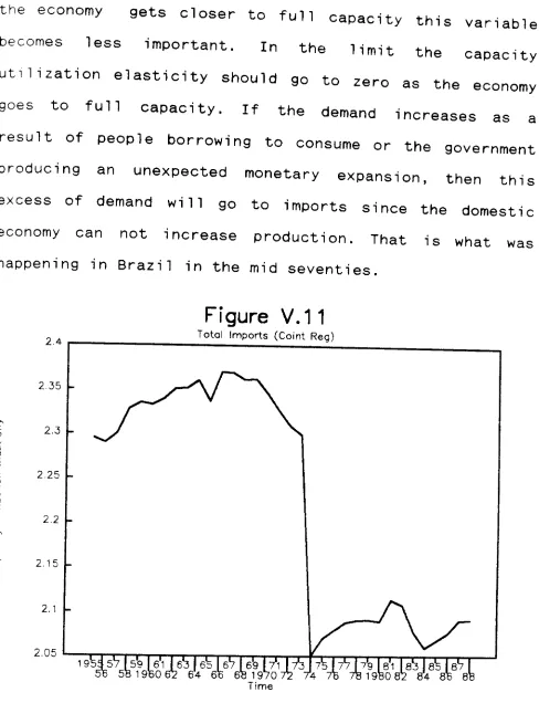
in the _{case of capacity utilization,} it has been _argued that _{a negative sign can} be _{seen as appropriate.} If the domestic business _cycle follows the same pattern as the world economy, then it seems possible that an increase in capacity utilization will lead to a reduction in imports, since domestic producers can supply faster than foreign ones. 11

Moreover, as shown by Barker (1979), since potential output is usually calculated as a function of time, these three _{variables are} interconnected. Despite the different economic interpretation that is given to justify the use of such variables, it seems that they are all capturing

the _{same phenomenon.} It is _{our view} that _variables such

10) See, for _example, Weisskoff (1979).

11) Akhtar (1981) _and Barker (1987) found _evidence of a

negative relation between capacity utilization and

as the potential _{product and} the time trend _may be

accounting for structural _changes in the demand for

imports that _{cannot be accommodated by the assumption}

of fixed _{coefficients.}

3.2) Export Eouations

Exactly _{as in} import _equations, it is _{also common to} include _{other variables such as capacity utilization,}

potential product or a time trend in export equations.

Goldstein _and Khan (1978) developed _{a model where} the potential product is one of the explanatory variables in the _{supply of exports.} The idea is that _{exports should} respond positively to changes in the country's capacity to produce. Their model, with some alterations, can be defined _as

*

1n Xd = ao + al 1n[ Px (1 +T* ) /Pd ]+ _a2 ln Y* (27)

In XS = bo + bi in [ EPx (1+S)/Pd ]+ b2 In YP

. (28) a2 , bi , b2 >0, a, <0

This _{model can also} be used to justify the _presence

of potential product, as well as other variables such as

capacity utilization, in the reduced form equation.

Solving (27) for _{Px we obtain}

*

ln _{Px = co + ci} ln _{Xd + C2 ln(} 1+T* )+ c3 1n Pd

+ C4 1n Y* (29)

where,

.

co =- ao /al _{, ci} /ai _{, c2} C3 =1, C4 a2 /al

C3

, C4 i 0, Cl , C2 <ý

Substituting (29) into (28) and assuming market

1nX=( _{bo + bi co ) /D + b2 /D In Yp + bi c4 /D}

In Y*

+ bi /D In [ EPd (1+S)/Pd(1+T* _)]

. (30) where, D=1- bi cl

Since D is _{positive, the}

coefficients _{are all}

expected to be positive. Similarly, _{one can get the}

reduced form for _{prices by solving (28) and (29) for Px.}

*

In Px = (co+ci bo )/D _{+ 1/D} In [Pd/(1+T* )] _{+ c4/D in Y*} + c1b2/D _{In YP + cibi/D} In [E(1+S)/Pd]. ₍₃₁₎ As noted above, one could use this same framework to introduce _{capacity utilization. It is normally}

argued that the _{supply of exports depends negatively on the} level _{of capacity utilization. The central argument is} that _{producers always serve the home market first,} because foreign _{markets are presumably less profitable} due to _{more costly marketing, transport costs or greater}

risk. Therefore b2 would be negative. Winters (1981) _and Hotson _{and Gardiner} (1983) _adopt this _approach.

unimportant and those influencing _{supply -} investment, profitability _- become _{suddenly all} important. " 12 In analytical terms the model can be described _as

x=

min (xi,

X2 )

xi = at (Yf, P/Pf) + bi q X2 = az (K, P/Ph) + bz q

p= cl (Pf) + di _q if _{x= xi} = c2 (Ph) + d2 q if x= X2

where, xi is the demand for _{exports, X2 is the export}

supply, Yf is real foreign income, K is the _{net stock of}

capital of the firm, P, Pf and Ph are the export price of

the firm, _{price of competing goods and home market price}

respectively, and q is the capacity utilization rate.

Taking _{an individual} firm, it _{has to be operating} in

the demand or supply constraint case, but for the economy

as a whole there can exist both demand and supply

constrained firms. Therefore for a firm there will be a

threshold _point (q') _where it jumps between _regimes, but

for the _{economy such} jumps _{are clearly} implausible.

Observations _cannot be fully _{characterized as} belonging

to _{one or} the other regime, but rather as helpful in

describing both _regimes. Obviously, _{one observation} will

tell _{more about} the _{supply constraint} case once µq, the

average of q for all firms, is less than q' and vice

versa.

Given _a distribution function for the capacity

utilization g(q), which has a expected value of µq, the

volume of exports for the _economy is (a _{similar equation}

could be written for _{export prices as well)}

+Co

X=x _g(q) dq

-ao

g' +ao

= xi g(q) dq + _{x2 g(q)} dq.

_Co g'

To make the model operational we just have to add a

disturbance term to the _{equations and specify the form of}

the distribution function _{g(q). One will then end up with}

a single equation that can be estimated by ordinary least

squares, being the parameters in both regimes retrievable

from this "reduced form". 13

A time trend has _also been _used in _{export models,} although its theoretical justification is sometimes not very convincing. In studies on the UK economy, the basic justification for _using time is the long term reduction in the UK's _{share of world exports.} 14 The idea is that British _exports have been _subjected to _a long term _non price loss of competitiveness, so that the coefficient on the time trend _will have _{negative sign.}

4) Some Econometric Considerations

When _estimating trade _equations, as in other

economic relations, one faces several econometric

problems, such as choice of functional form,

13) Another approach to the estimation of this problem based in _{switching regressions} is suggested by Goldfeld and Quandt (1973a and 1973b).

14) See, for _example, Dinenis et alii (1989) or 3rooks (1981).

simultaneity, dynamic _{specification, stability of the} parameters and aggregation _problems.

4.1) Functional Form

Almost _{all empirical work on trade equations is} based _{on a} log linear _{specification.} The _evidence in favour of the log linear _{specification} in import demand was first provided by Khan _and Ross (1977) _and later confirmed by Boylan et alii (1980), both _using the Box and Cox methodology. More recently Hitiris _and Petoussis (1984), _{using a methodology} developed by Godfrey _and Wickens (1981) that _allows for _{serial correlation, again} come out in favour of the log linear specification. In terms _{of export equations,} this _problem has _normally been dealt _{with by assumption.}

4.2) Dynamics _{and Stationarity}

To _account for the fact that the full _{response of} the dependent _variable to _changes in the _explanatory variables may not be completed in the same period, different dynamic _models have been _used. Perhaps the two most popular ones are the partial adjustment and the polynomial distributed lag models.

Although the _use of dynamic specifications seems essential when working with quarterly data, the evidence suggest that _most of the adjustment occurs within a year.

Goldstein _and Khan (1976,1978), for example, have

estimated that the average lag of total imports is

between _{one and} five _{quarters. If}

one is considering disaggregated data, _{the problem}

can be more _complicated once some goods, especially _{capital goods, are subject to}

longer delivery lags.

Another _{noteworthy observation is that}

normally a "specific to _{general" approach has been}

adopted. It is common to start with simple models that _{are subsequently} expanded to solve the _{problems that emerge. As shown by} Hendry _and Mizon (1978), this is _{not the most adequate} way to proceed, once the test _performed in the _{new model}

is _{conditional on the result of the tests done in the} former _model. 15

A more adequate and elegant way of dealing with the

question of model dynamics is to _{adopt an error}

correction model (ECM). In the ECM the _{estimation of the} long _{and short run coefficients} is done _separately. The long _{run coefficients, also called cointegrating vector,} are obtained in a first stage by either the Engle _and Granger two _{step method or} the Johansen _procedure. These coefficients are then used in the _{second stage when only} the _{short run responses are estimated. This will be the} approach used in this thesis. 16

In _addition, the ECM is _{also a good answer} to the

question of non stationarity. All the empirical work on

the Brazilian trade _equations have _assumed, implicitly,

15) An _exception is Hitiris and Petoussis (1984), who adopt a "general to specific approach".

that the _{variables of interest}

are _{stationary. 17 If the}

variables are non-stationary but _{cointegrated then the}

ECM is the proper _{model to use. 18}

4.3) Simultaneity

As _{noted above} it has been _{more common to use}

simultaneous models for _{exports, using the "small}

country" hypothesis to justify _{the estimation}

of the

demand equation alone in the _{case of} imports. _{A better}

procedure, however, _would be the _{specification of a}

complete model that could be tested for _{price exogeneity.}

Although the _simultaneity between _{prices and}

quantities is _{ruled out by the "small country"}

assumption, simultaneity can still be a problem in

relation to imports _and income. Considering _{an extended} model, the level _of imports _{can be seen as an explanatory} variable in the income _{equation. This is especially true}

in _{the case of essential imports. For a country where} essential goods represent a large proportion of total

imports, _{a simultaneity problem should be expected even} in _{the total imports equation. Most of the literature} ignores _{this problem, failing to even test for the} endogene i ty of income. 19

17) The _{unit root} tests _{carried out} in _{chapters 5 and} 6 show that _all Brazilian series used in the estimation of trade _{equations are} indeed _{non-stationary.}

18) See Engle _{and Granger} (1983).

19) Exception is Moraes (1986), _{who estimates a}