Master Thesis
Single-to-many Dynamic Traffic Assigment for
Container Freight on a Multimodal Network
Abstract
This research presents a mathematical programming formulation for a Dynamic Traffic Assignment model and an implemented iterative shortest-path algorithm. Freight transport demand is assigned to a dynamic network of roads and waterways with the goal to minimize transportation costs. The challenge is to assign paths to a network with time-varying travel speeds and capacities, the assignment of limited capacities to different freight shipments and determining of travel and waiting times. Assigning on a multimodal and dynamic network lead to a non-classical shortest path problem.
Preface
This master thesis is the final assignment of my study Applied Mathemathics at the University of Twente. The specialization of my masters’s programme is Operations Research and this thesis was done for the group Discrete Mathematics and Mathematical Programming.
TNO
I did this research at TNO, which is an independent research organization. The mission of TNO is to connect people and knowledge to create innovations that boost the sustainable competitive strength of industry and well-being of society. For this master thesis I did an internship at the Sustainable Transport and Logistics deparment of TNO.
At this department a model has been developed that can assign freight from the Port of Rotterdam to a final destination in the hinterland. This model is used to analyse multimodal and synchromodal transport flows and the effect that route and mode choices have on emissions and the accessibility and safety of the network. The downside is that this model assigns onto a static network, meaning that all travel information is based upon daily averages and there is no specific record of at what time each shipment is where in the network.
Acknowledgements
I would like to thank everyone that supported en guided me during this master thesis.
Prof. dr. Johann L. Hurink
For being my supervisor for this thesis, the valuable converstations we had on the mathematical problems at hand and the guidance for writing this thesis.
Dr. ir. Mo Zhang
For iniating this master thesis from within TNO, being co-supervisor for the first four months of my internship and increasing my knowledge on Transportation Research.
Layla Lebesque MSc.
For replacing Mo, therefore being co-supervisor for the remainder of my internship and for the guidance in finishing this thesis.
Dr. G.J. Still and Dr. J.C.W. van Ommeren
For completing my graduation committee and taking the time to assess this master thesis.
Colleagues at TNO
For a really nice atmosphere and all conversations which contributed to my internship and the quality of this research.
Family and friends
Contents
1 Introduction 6
2 Problem statement 8
3 Literature review 10
3.1 Transportation research . . . 10
3.2 Iterative path choice . . . 14
4 Mathematical Model 18 4.1 The problem . . . 18
4.2 Input . . . 19
4.3 Mathematical program . . . 21
5 Approach 28 5.1 Shortest-path problem . . . 28
5.2 A* algorithm . . . 31
5.3 Non-classical shortest-path problem . . . 34
5.4 Waiting-time expansion . . . 36
5.5 ICPA* . . . 38
6 Implementation 39 6.1 TransCAD . . . 39
6.2 ICPA* implementation . . . 40
6.3 Verification . . . 44
6.4 Calibration . . . 50
7 Use case 57 7.1 Parameter choices . . . 58
7.2 The case . . . 58
7.3 Results . . . 62
8 Conclusion and recommendations 66 8.1 Conclusion . . . 66
8.2 Recommendations . . . 67
References 72 Appendix 72 List of symbols and list of abbreviations . . . 73
Mathematical program - Single Cheapest-path Problem (SCP) . . . 75
1
Introduction
Freight transport around the globe is continually increasing. This growing amount of transport requires more capacity of available infrastructure. Consequential larger networks and more interacting trade routes require more and better transport planning. The search for cost reduction and increasing efficiency on these larger and more complex systems has driven research on transport planning. This is resulting in more complex problems, which are getting harder to solve.
Transport planning takes place at three different levels: Strategic, Tactical and Operational Planning [33]. Strategic or long term planning involve highest levels of management and deal with major capital investments, mainly physical network building or resizing. Tactical planning aims at the allocation of resources and scheduling services on a medium term horizon, such that system performance is improved. Operational planning deals with all short term decisions on transport activities: scheduling of services, maintenance, crews and routing of vehicles. This research focuses on routing vehicles and therefore fits in the level of operational planning.
A decent operational planning is required to minimize costs and optimize the amount of freight demand that can be satisfied. A better planning increases the efficiency of system. The optimization of the planning lies in making efficient schedules for vehicles, ships, operations, crew and all other factors that complete the system. To be able to make an efficient planning for all these parts of the system it is required to know what freight has to be transported at what times.
This research focuses on optimizing the operational planning for the transport of shipping containers from the port of Rotterdam to destinations in the Benelux or Germany, the so called hinterland. The challenge is to plan a route for each freight shipment. This planning of routes involves the scheduling of which container will be transported by which vehicle or vehicles to get from Rotterdam to its final destination. It also involves the routing of these vehicles over the transportation network. These vehicles having limited capacity, leads to a challenge of which shipments to assign to which vehicle. The vehicles considered in the setting are trucks and barge ships, also called the transport modalities or modes. The created model can also be used for different types of goods than containers, if vehicles are considered which can transport those goods.
schedules dealing with the transportation of these freight shipments. This is where the Dynamic Traffic Assignment model comes into scope, to be able to assign routes to freight traffic in a dynamic situation.
The goal of this research is to make a tool that can find a dynamic freight traffic assignment that allows all freight demand to be delivered succesfully. The tool should be able to assign freight orders to vehicles and routes and therefore be able to make a decent route schedule. Making such a decent schedule requires to know the travel times and capacities of the vehicles on the dynamic network.
2
Problem statement
The main problem considered in this research is optimally assigning freight transport onto a dynamic traffic network. The transport network is dynamic, which means that the best route from an origin to a destination is not always the same. Travel speeds on roads can fluctuate and capacities of barge ships and terminals are limited. External influences such as rush hour or network disruptions, by accidents or breakdowns, can also change the best routes. Furthermore, the already assigned freight shipments also influence the network, because they can increase rush hour congestion or use the limited capacities of terminals or barges.
To be able to determine the routes that minimize costs it is required to know the availability and transport times of vehicles. However, as mentioned before the travel speeds and capacities vary over time. So for finding the total travel time of a route it is necessary to know which vehicle(s) can be used and the travel speed of the vehicle(s). The determination of travel times based upon time varying travel speeds adds the time dimension to the routing problem. This time dimension can lead to computationally heavy route calculations. However, in practice the choice of a route often has to be done reasonably fast, to make response based upon real time information useful.
The goal of this research is to create a Dynamic Traffic Assignment (DTA) model which allows to find the cheapest routes, based upon time dependent network data. To react on real-time information it is necessary that a solution should be found in a reasonable amount of time, as this would make real-time response possible, e.g. route improvements along the way. This leads to the following question to be answered by this research:
• How can a Dynamic Traffic Assignment model effectively assign dynamic freight
demand on inland waterways and roads dealing with disruptions and congestion?
To be able to answer the research question the following subquestions are formed.
• How to find dynamic routes fast enough to make real-time decisions?
• How to assign freight demand requests to limited barge capacity?
• What insight in network behaviours could a dynamic traffic assignment model give
The first subquestion focuses on the time required to find a dynamic route. If some disturbance occurs, then some route might be blocked and routes would have to be changed. It would be useful to assign new routes within a certain amount of time. To do this new routes have to determined fast enough. Finding these routes fast enough contributes to the DTA model.
Barge ships have the capacity to transport many containers and can therefore carry different freight demand requests simultaneously. Making a decent planning for putting the shipments onto the barge ships can make sure that the barge ships are used efficiently. The DTA requires freight to be able to be assigned to barge ships and so this assignment of freight onto the ships is part of the research problem.
Next to having a model that can be used to make a traffic assignment for freight onto a dynamic network, it is good to recognise the practical insights that can be retrieved from a resulting traffic assignment. To show application possibilities of the model this last subquestion is defined. Furthermore, the DTA model should be able to give insight in freight traffic behavior and economic effects of network disruptions. It might even be used to give insight in the robustness of the traffic network.
3
Literature review
In this section a literature background on transportation research is given. The basis of transportation modelling and the more recent developments on (dynamic) traffic assignment problems are mentioned. Also a background on shortest-path problems is given as this has also been used for this research. In the remainder of this report, the term ’path’ will be used instead of ’route’, because the transportation network is considered to be described by a graph and in graph theory it is common to refer to paths instead of routes.
3.1 Transportation research
This subsection focuses on the basics of traffic assignment.
3.1.1 Operational planning
There are several levels of planning in transportation research, as mentioned in Chapter 1. This research mainly deals with the operational planning level of transportation research. Strategic planning might come into scope when more long-term elements such as available vehicles or network changes are considered. On an operational planning level studies have been done on reducing travel times and transport costs for given sets of transport requests. Most studies consider the situation where the path choices influence the costs or even the possible paths for other traffic. In these cases the goal is to find some equilibrium, meaning a solution where it is not possible to improve the current situation. The equilibria in transport modelling are known as the principles of Wardrop [37].
3.1.2 The principles of Wardrop
There are two main types of equilibria in transportation modelling. One equilibrium minimizes the average travel costs per user or equivalently the total costs of the system. This is known as Wardrop’s second principle and called the system optimum (SO) or a system-optimal equilibrium. The other equilibrium is known as Wardrop’s first principle and is called the user equilibrium (UE), this specifies a situation where no single user can find a cheaper path, if all the users stay at their current choice.
3.1.3 Modelling methods
There are several different modelling methods that are used in transportation modelling. The studies for optimizing tranportation systems on an operational level can be categorized in four broad categories. The categories are mathematical programming [23], optimal control [13], variational inequality [24] and simulation-based approach [12] [22] [34].
Mathematical programming and optimal control approach a traffic assignment problem with a similar goal function and constraints. The main difference is that the mathematical programming approach uses a discrete-time step where the optimal control constraints are defined in a continous-time setting, resulting in a continuous-time optimal control problem [33]. Merchant and Nemhauser [23] formulated a mathematical program which has been used as a basis for other studies on dynamic traffic modelling [5] [10] [36].
The mathematical theory of variational inequality was developed to solve equilibrium problems. As such, it can also be used for a traffic flow equilibrium problem. Several algorithms and solution methods have been developed to deal with inequality problems [24]. Finding a suitable solution for a traffic assignment problem is often not very efficient, as it can take quite a lot of time to find a equilibrium. It can also be difficult to calibrate model parameters to get a realistic and practical solution. In these cases a simulation-based approach could be useful. Creating a simulation model can result in more practical results. However, a simulation does not guarantee that some optimum or equilibirum is found. A method to bring a simulation-based model closer to an equilibirum is the Method of Succesive Averages (MSA)(see section 3.1.4).
The above described methods are different in the mathematical approach, but they all may be used to represent traffic situations. For this they use similar representation to describe a transportation network or the behaviour of traffic flow. The main aspects of this modelling of traffic flow are described in section 3.1.5.
3.1.4 Method of Succesive Averages
It can be hard to find an equilibrium when using a simulation-based approach for a traffic assignment problem. Especially a SO can be hard to find. Most simulation-based approaches try to improve the traffic situation step-by-step until a equilibrium situation is found. MSA is a method to improve such a search for an equilibirum.
behaviour of a simulation-based model hard to track and it is therefore difficult to guarantee convergence of such an iterative procedure [34].
MSA is an effective solution heuristic that has been implemented in simulation-based DTA models. The basic idea behind MSA is that in each iterative step all possible cheaper paths are determined, but only a part of the flow is assigned to these cheaper paths. The advantage of only rerouting part of the flow is that the cost effect for the other flows also occurs only partially. If the made changes seem to be a step in the right direction, then the method records that the change in this direction was succesful and will do more steps with the same direction.
3.1.5 Traffic flow modelling
In the subsections above possible approaches for traffic models are considered. All these approaches have in common that they need to determine the travel costs of specific flows to be able to minimize the costs of travelling over a network. In general, the travel costs per link are considered, which depend on the travel time and some other travel cost. Furthermore, the amount of time it takes to traverse a link is physically dependent on the length of the link and the speed of travelling, whereby the travel speed can vary through time in a dynamic network. An aspect that comes into scope with dynamic traffic flow modelling is the order in which traffic enters and leaves the link.
The travel speed on a link can depend on the amount of flow on the link, e.g. the decrease in travel speed on a road when rush hour congestion occurs. When more traffic is using a link, then the speed on that link decreases until some critical amount of flow is reached and congestion occurs. Therefore, the traffic flows have to be integrated into a model to take this effect into account. This can be done in several manners.
3.1.6 First in, first out
In traffic flow modelling there is some order in which traffic enters and leaves a link. In static modelling the time a vehicle enters or leaves a link is not taken into account. However, in a dynamic model the time of entrance and exit of a link do get attention. For a single lane traffic link it is clear that in reality a vehicle leaves the link before the vehicles that entered the link behind him, because it is not possible to overtake on a single lane. However, for multiple lanes the situation may be different and vehicles may overtake ieach other. The non-overtaking property is also known as the First-In-First-Out constraint (FIFO). This FIFO policy, which is also known from warehousing or inventory problems, can be integrated into traffic models if the given application aks for it.
There are different methods of implementing FIFO for the different mathematical approaches. Most methods deal with some restriction or constraint for flow or travel time. If FIFO constraints are added to a variational inequality formulation, then it is no longer sure that a solution continues to exist [10]. It is also possible to add FIFO constraints to a mathematical progamming model [3], but it results in nonconvexity issues. Furthermore, if a continuous time formulation with FIFO constraints is studied, it also results in nonconvexity for the objective function [3]. Thus the FIFO policy can be integrated in the different mathematical formulations, but the consequential nonconvexity complicates searching for solutions.
In the continuous approach no new variables and fewer constraints are necessary to integrate FIFO, compared to the discrete case. It is not necessary to add direct FIFO constraints, because of the continuous time setting. Assuming the speed is the same for all flow on a link, then there never is a speed difference between seperate flows on a link. Having the same speed implies that a flow can not pass any other flow on the same link and thus the FIFO policy is followed.
A method to ensure FIFO via the link travel times is to smoothen the travel speed function, where the travel time is determined upon the link travel speed function at time of entrance [11]. The method used in the implementation of this research to ensure FIFO on road links is based upon a method by Ichoua [18]. The method puts constraints on the travel time over a link. These constraints ensure that the travelled distance over the link is at least the length of the link, see section 4.3.4 for further explanation.
3.1.7 Freight assignment
that there is also other traffic on the network. Assigning only a part of the flow implies that the total flow is not known and a corresponding flow speed cannot be determined directly.
The mentioned property, that we assign only a part of the traffic flow, makes this research different from most DTA problem, because only a part of the network flow is known. The unknown part of network information may get specified by input distributions, similar distributions for the network state have also been used by [9] and [28].
3.2 Iterative path choice
As mentioned in the previous section the network state is not directly known when the assigned freight flow of a traffic system is only a part of the total trafffic. In this situation we could have the network state as some given input. This would allow different ways of finding a path for each freight order instead of modelling traffic flows. One possibility is using a shortest-path algorithm to find a shortest path from origin to destination for each shipment. If the travel time of links is used as input for a shortest-path algorithm instead of the length or weight of the links, then it is possible to use such an algorithm to find a fastest path in a dynamic network with FIFO consistency [9].
Individually finding a cheapest and possible path for each freight order could be a decent solution for the traffic assignment. However, if the assigned paths have some influence on the network state and therefore some influence on the path choice of other freight orders, then this approach only approximates the real situation. If this influence could be constrained in such a way that costs of already assigned paths are not influenced, then it could be possible to iteratively assign cheapest paths to find a UE. That is because iteratively picking a cheapest path and not influencing costs of earlier picks, implies that no freight shipment could have picked a cheaper path.
Iteratively assigning cheapest paths has been applied in literature and also in this research to find a solution for a DTA problem. The following sections describe the development of shortest path algorithms and their use in dynamic networks.
3.2.1 Static shortest-paths
The most famous algorithm for finding a shortest-path between 2 vertices of a graph is the Dijkstra algorithm [8]. The algorithm builds a shortest-path tree from the start node until the goal node is found. A downside is that this method is computationally heavy for large networks.
the A* algorithm [16]. This algorithm uses a guiding heuristic function to direct the search towards the destination. Where Dijkstra’s method builds a shortest-path tree from the origin in all directions, the A* method only computes the shortest-path tree from the origin towards the destination. This requires that some positioning of nodes in the network is known, e.g. locations in an infrastructure network are positioned on a map, on this map the Euclidean distance between nodes can be determined. This Euclidean distance is a possible heuristic funtion that can give the A* algorithm a search direction. With the heuristic the algorithm constructs a smaller shortest-path tree before it reaches the goal node, compared to Dijkstra’s algorithm. Note that the performance of A* depends on the quality of the heuristic function and there are several conditions that the function must satisfy [20].
A newer and computationally faster method for determining shortest-paths on road networks is the reach-based method. The paper of Gutman [14] describes this algorithm and gives a comparison between the performance of Dijkstra, A*, Reach, Reach combined with A* and Exact Reach. The reach-based method is computationally faster than the A* algorithm if the algorithm has already preprocessed the network. However, this preprocessing takes quite some time. As a consequence only if the number of the to-be-assigned paths is large enough then the total computation time required by the Reach algorithm is less then the total computation time required by A*.
3.2.2 Dynamic optimal path choice
The shortest-path algorithms are initially made for static graphs, so they had to be altered to able to find a fastest paths in a dynamic network. One of the first papers on dynamic path choice was [6]. An iterative scheme is devised to compute a shortest path in a network with time dependent transit times. It originates from Bellman’s iteration scheme [1], which was based upon his principle of optimality.
One of the first papers on a minimum-time-path algorithm for a network with time-varying link travel times has been written by Dreyfus [9]. He states that Dijkstra’s algorithm can be used to find a shortest travel time path in a time-dependent network. Orda and Rom [28] made a general analysis for a shortest-path algorithm for a network with time-dependent link delays, which is similar to link travel times being time dependent. They conclude that efficient solutions exist if waiting at a node is only allowed at the source node, general waiting contraints for all nodes make the problem very complex. Hall [15] states that Dijkstra’s algorithm does not find minimal expected travel time paths if stochastics are introduced into time-dependent travel speeds and travel times.
paths taking into account time-varying link speeds and subsequent link travel times. This method assumes that time dependent travel times estimates are known.
3.2.3 A* algorithm with dynamic link weights
The A* algorithm will be used in this research, because the dynamic link weights complicate the problem and therefore a initially faster shortest-path algorithm has not been used. Reversed search from destination to origin has not been used because the starting times at links are required for determining the travel costs. A preprocessing algorithm is not used because of the dynamic network. Preprocessing would have to be done for a lot of(or all) time steps and when capacities or travel speeds change then the network also changes and preprocessing has to be revised.
The A* algorithm has been used before with dynamic link weights. Horn[17] used the A* algorithm with varying travel times as link weights, the travel times were required to be FIFO-consistent. In the problem of this research we will have costs as the link weights, they would also require similar consistency to have A* function properly.
3.2.4 Time-Expanded network
Another method of dealing with a dynamic network is by using a Time-Expanded network [5] [27], or also called Space Time Network [29]. A Time-Expanded network can be created by partitioning a time horizon in a number of discrete periods and duplicate the nodes, such that each node is represented in all time periods. The link traversal times are rounded to a corresponding number of time periods and the given links (i, j) are duplicated and now connect nodes i and j in different time periods. More precisely, links (it, jt0) are created
where it denotes nodei at time period t, node jt0 denotes node j at time t0, where t0 −t
equals the travel time fromitojat timet. Now the Time-Expanded network can be seen as a static graph and a static shortest-path algorithm can be used to find a path in this graph.
A disadvantage of this network propagation is that an already large network gets even larger, as the number of nodes and links get multiplied by the amount of time expansions. This decreases the tractability of the cost minimization problems. Ziliaskopoulos and Wardell [39] confirm that time expansion is computationally expensive for large networks and therefore usually impractical.
3.2.5 Multimodality
4
Mathematical Model
In this section a mathematical program is formulated. The objective of this program is to find the best solution for the DTA problem. First some required assumptions are described and afterwards the input, to-be-made decisions, constraints and objective function are put into a mathematical framework. This framework is only used to formalize the problem and it is not a model that can be used directly by a solver.
4.1 The problem
The problem considered in this thesis is to find cheapest paths for freight orders from a single origin to several destinations in a given network. For this mathematical formulation paths are denoted as a series of connected links in the transport network, because each link adds some link specific costs to the total path.
Freight can be shipped by two different transport modes, road and waterway. To model the behaviour of these transport modalities some assumptions have been made.
The first assumption (4.1) states that trucks from assigned freight orders do not influence the time dependent travel speeds of road links. In general, the travel speed on the road is dependent on all traffic on the road and not only the assigned freight trucks. The main reason for making this assumption is that in the real situation on most roads the fraction of trucks assigned by the considered traffic assignment problem is small. This implies that the rest of the flow (all other traffic) mainly determines the speed of travel.
Not making this assumption would imply that the travel speeds are influenced by the assigned freight. To determine this influence the total flow of the network should be taken into account. Then it would be possible to determine the effect of the assigned freight on the total flow and the consequential travel speeds. To do this would require distributions of network flow through time. However, these are not available as input and modelling the entire network flow would really increase the level of complexity of the model.
The travel speed distributions are considered to be input. These distributions are considered to be based upon some expected amount of traffic on the network. In this expected amount of traffic there is also some expected amount of freight traffic. The better the freight assignment meets these expectation the more realistic the travel speed distributions are, if all other flow behaves accordingly.
The next assumption (4.2) is made to be able to model the assignment of freight orders onto barge ships. It is assumed that barges sail a predetermined path defined by a predetermined schedule and each barge has a specified capacity. It would be more realistic if the model could also schedule the paths sailed by barges. However, it turns out that this assumption is necessary to be able to develop an efficient solution method (see Chapter 5). Determining the paths sailed by barge ships and the sailing times is considered to be a seperate optimization problem, which will not be treated in this thesis.
Assumption 4.2 Waterway links are sailed by barges on a predetermined schedule, each barge has a specific route, sailing times and capacity.
4.2 Input
In this section all input for the considered dynamic freight traffic assignment problem is specified.
4.2.1 Time horizon
The time dimension has to be taken into account, because we are dealing with a dynamic problem. We define T to denote a point in time, t to denote an amount of time and T a time interval. All T considered in the model will be in the time interval Thorizon. This interval will be referred to as the time horizon and is defined by a starting point T0 and an end pointTend: Thorizon:= [T0, Tend).
For later purpose we define all T to be integer. Subsequently, t defined as the difference between two points in time is also integer.
4.2.2 Network
The freight demand needs to be assigned to paths. These paths should be found in a traffic network. Therefore a traffic networkG(N, A) is given, whereN is the set of nodes andA
is the set of directed links of the network. Each node represents a geographical location and can be either a centroid, a terminal or a junction of links.
• A centroid represents an origin or destination of freight.
• A terminal is a location where freight can change from transport modality, e.g. at a terminal containers can be loaded from a barge onto trucks.
• A junction is a node where several links of the same modality are connected.
of the following three subsets: roadsR, inland waterwaysW and virtual linksV. For each linkawe have link length La, freight flow capacityFaand costscFa. Virtual links are used
to include multimodality in the model, see 3.2.5.
• A virtual link connects the node of a transport modality to a terminal node. These links are used to take into account the time it takes to (un)load a truck or barge and also the capacity and working hours of the terminal.
• Road and waterway links represent the real world roads and waterways.
For later use, for each node we define sets of links that contain all links entering and leaving the specific node. For each nodei∈N,Aini contains all links directed towards iand Aouti
the links directed out of node i. Formally, Aini := {a | a ∈ A, j ∈ N, a := (j, i)} and
Aouti :={a|a∈A, j ∈N, a:= (i, j)}.
4.2.3 Truck travel speeds
Assumption4.1implies that travel speeds on roads are not influenced by assigned freight. Therefore the travel speeds for trucks on the given network are considered to be given as input. These input travel speeds are time dependent. As T ∈ Thorizion are integer
values these travel speeds are specified by vectors. For every road link a ∈ R the vector isva = va(T0), va(T0+ 1), ..., va(Tend−1)
. Where va(T) defines the travel on speed on
linkaon the interval [T, T+ 1).
4.2.4 Barge schedule
This section describes how the model can assign freight demand to travel by barge ships. A barge schedule is considered to be a given input by assumption 4.2. Hereby, the paths sailed by barges, the interarrival times at nodes along the path and the capacity of each barge are given.
A barge can only be loaded and unloaded at a terminal. This means that if a freight shipment is loaded onto a barge at some terminal that this shipment at least stays on this barge until the next terminal that is visited by this barge. For freight shipment only the travel time from terminal to terminal and the capacity of the barge are important.
with departure timeTadepartureand arrival time Taarrival for a single barge.
This setB will now be considered as part of the traffic networkG(N, A) and therefore part of the set of linksA.
4.2.5 Link capacities
For virtual links a∈V a remaining capacityFa(T) is defined for allT ∈Thorizon and for
each barge linka∈B a capacity ofFa is defined. This barge capacity has no time variance
because the capacity is used for the entire link with an already specified time window:
Tadepartureuntil Taarrival. Road links have no capacity constraints.
4.2.6 Travel costs
The goal of the assignment is to minimize the transportation costs. The transportation costs are determined by a direct cost factor per linkcfa, a travel time cost factor per link ct
a and a waiting time cost factorc t,wait
a . All these costs are per unit of freight.
4.2.7 Freight demand
Now only one input for the model is left to describe, which is the freight demand that has to be assigned. The freight demand is given and specified by set1 OD. Each freight demand d ∈ OD defines a transport request of Fd units from an origin node Orid to a
destination nodeDesd with release timeTdrelease.
4.3 Mathematical program
In the previous section we have defined the given input. For this input we want to find the cheapest paths for all freight demandd∈OD. In the following a mathematical program is formulated, which can be used to solve this cheapest path problem. For this mathematical model, decision variables, constraints and an objective function are defined in the following subsections.
4.3.1 Decision variables
The general goal is to find a cheapest path for each freight order. So for eachd∈OD we want to find a series of connected links which form a pathPdfromOrid toDesd. We have
to determine which links are used for such a path. Another decision to be made is the time schedule for using the path. This means that we have to determine when the freight transport starts and when and how much waiting time to take at nodes along the path.
1
Note, in this model waiting is only possible at terminal nodes and the first node Orid is
a terminal. In reality it might happen that a barge with oil is ordered to wait along the route, because fluctuating oil prices can make this profitable.
Now we define decision variables which can be used to determine the cheapest path including the required departure times. To assign a specific path consisting of linksa∈A
to a freight shipmentd∈OD we define an indicator variableδd,a. This variable indicates
if a link is in Pd or not. This choice for a decision variable on link level is made to be
able to define total costs of paths and define flow constraints. For waiting at a terminal an integer variable waiting timetwaitd,a is introduced and for travelling over a link an integer variable for travel timetd,a is introduced for all links a∈A and freight demandd∈OD.
td,a, twaitd,a ∈Z+.
δd,a∈ {0,1}, δd,a = 1 ⇔ a∈Pd.
4.3.2 Constraints
The constraints are split up in 3 different groups; routing contraints, capacity contraints and time constraints.
4.3.3 Path Constraints
The path constraints have to make sure that for eachd∈Dall a∈Awhich haveδd,a= 1
form a pathPdbetweenOridandDesd. First we have to make sure that the path originates
atOrid and ends atDesd. Furthermore, to ensure that the path is connected, a constraint
is added to make sure that each node n where a link enters also a link leaves node for
n6=Oridand n6=Desd. This results in the following contraints:
X
a∈Ain i
δd,a−
X
a∈Aout i
δd,a =
−1 i=Orid.
0 ∀i∈N 6 {Orid, Desd}.
1 i=Desd.
(1)
It is possible that a path through the network contains a cycle. In a cycle at least one node would have more then one entering link. However all travel times and direct costs are positive. This implies that a cycle will never be in a minimal cost path.
4.3.4 Travel time constraints
As travel times on links are time dependent, we need to know at what time each link is entered. This time of entrance depends on all foregoing travel and waiting times, and the initial release time. To model this, let td,a denote the travel time for link a ∈ A and a
shipment d∈D and letTd,ain denote the entrance time of link a∈ A for shipment d∈ D. All these variables are integer within the time horizon Thorizon and they are defined by the following equality constraints. Where the entrance time of the next link a is defined as the sum of the entrance time of the previous link, travel time on the previous link and the variable waiting time before entering the linka.
Td,ain =
twaitd,a +δd,aTdrelease ∀a∈AoutOrid.
twaitd,a +P
a0∈Ain i δd,a
0(Tin
d,a+td,a)
∀i∈N/{Orid, Desd}, a∈Aouti .
0 ∀a∈AoutDes
d
(2)
These constraints are quadratic, because of the multiplication of variables. It is however possible to rewrite these quadratic equality constraints to linear inequality constraints. To do this we first define a large numberM, with−M < T0 and M > Tend. With this large numberM we define linear inequality constraints that ensure allTd,ain satisfy the contraints above. The variableTd,ain should equal zero if the linkais not used by freigthd, equivalent toδd,a= 0.
This first linear contraint ensuresTd,ainequals zero if the indicatorδd,a= 0. Ifδd,a = 1 then
this constraint would allow Td,ain to take any value between 0 andM.
The second and the third inequality contraint ensure that, if δd,a = 1 then the entrance
timeTd,a of linka is larger or equal the previous entrance Td,ain0 plus travel time td,a0 and
waiting timetwaitd,a . Note that there can only be onea0 ∈Aini for which Td,ain0 is larger than
zero, because there can only be one link entering the node i between a0 and a. If the indicator variable of link a equals zero then these constraints require Td,ain to be at least larger then−M, which is always true because Td,ain ∈Thorizion.
The fourth constraint below is required to ensure the equality of the contraints above.
Td,ain should be equal to the Td,ain0 added with twaitd,a0 and td,a0 of predecessing link a0. This
constraint is added to ensure the equality for links a and a0, leaving and entering some nodei.
Td,ain ≤δd,aM
Td,ain ≥twaitd,a +Tdrelease−(1−δd,a)M ∀a∈AoutOrid. (3)
Td,ain ≥twaitd,a +Td,ain0 +td,a0−(1−δd,a)M ∀i∈N, a∈Aouti , a0 ∈Aini .
Following constraints define the travel timestd,a for the different modalities. The decision
variables δd,a return in these constraints, because the travel time for unused links should
be equal to zero. As links that are not used should not influence the objective function.
Travel time on virtual links
Let αt
a denote the time to transfer one unit of freight via link a and let βa be the basic
handling time for a freight shipment. Then the travel on the virtual link is defined as.
td,a=δd,a αtaFd+βa
∀a∈V. (4)
Furthermore, terminals have specific operating hours, during these hours of the day containers can be processed. These operating hours are modelled in the capacity contraints, which will be specified later.
Travel time on roads
The time dependent travel speedsva on all road linksa∈R are given. Ichoua [18] defines
a method to deal with these varying travel speeds in a discrete time setting. This method puts a constraint on the travel timetd,afora∈R. The constraint makes sure that enough
time is spend on road linkato travel the total distanceLawith travel speed from vectorva.
Initially with Ichoua’s method the travelled distance on road linkais defined by summing the travelled distance in discrete time periodsτi. These periods are defined by a an amount
of time ∆τ: τi = [Ti0, Ti0+ ∆τ), τi+1 = [Ti0+1, Ti0+1 + ∆τ) = [Ti0+ ∆τ, Ti0 + 2∆τ). The
amount of time ∆τ and the travel speed during period i beingv(Ti0) imply the travelled distance in intervalτi equals ∆τ v(Ti0). The next equation defines the constraint where the
summation over periodsτi should ensure that the total link lengthLa is travelled.
X
τi
∆τ va(Ti0)
≥La ∀a∈R. (5)
Now we make a constraint from this inequality. The travel times in the assignment problem are considered to be integer, therefore the width of the time periods ∆τ is considered to equal 1. The first time period of a freight shipmentd∈ODon linkatherefore starts atTd,ain
and the travel time td,a determines the upperbound of the summation. This upperbound
will be Td,ain +td,a. The constraints should only set a travel time for links in the path Pd.
Therefore the distance to be travelled will equal the link length La multiplied with δd,a.
The resulting constraint for the mathematical program is.
Td,ain+td,a
X
t=Tin d,a
va(t)
As the given travel speeds are all positive, there always exists a minimalt∗d,afor eachdand
a∈Pd that satisfy this contraint for given value of Td,ain. All travel speeds being positive
implies that the constraint is also satisfied for all td,a ≥ t∗d,a. However, minimizing the
travel time costs is part of the objective, which implies that the model favors the minimal
t∗d,a.
Barge travel times
The set of barge linkB has been added to the network. Each barge linka∈B has a fixed arrivalTaarrival and departure timeTadeparture. The resulting constraint for the travel time
on barge linksa∈B is:
td,a=δd,a(Taarrival−Tadeparture) ∀a∈B. (7)
4.3.5 Capacity constraints
The capacity contraints have to ensure that the amount of flow on a link does not exceed the input boundaries Fa for a ∈ B and Fa(T) for a ∈ V. Assigning a path to a single
freight shipment d∈OD requires that at leastFd capacity is available on the links. This
means that the following constraints have to be satisfied.
δd,aFd≤Fa(T) ∀a∈V, T ∈[Tain, Tain+td,a). (8)
δd,aFd≤Fa ∀a∈B.
4.3.6 The objective
Now that we have defined all variables and constraints, what is left to do is to define an objective. First an objective function for a single freight demand problem is formulated.
For single freight demand d ∈ OD the goal is to find a cheapest path Pd. This means
that the costs of the resulting path should be minimal, where the total cost for a path is the sum of direct costs and time dependent costs for using links. We have the cost factors
cfa, cta, c t,wait
a . Time variables td,a and twaitd,a denote the time travelled and waiting time on
link afor freight d. Freight demandd has shipment size Fd and the path will be defined
by decisions variables δd,a and twaitd,a .
The objective function is below this paragraph, the following steps lead to this function. All cost factors are defined per unit of freight, so therefore the sum representing the path costs for 1 unit of freight is multiplied with Fd. The sum consists of direct link costs and
time dependent link costs. The direct link costscfa have to be paid if the link is part of the
the freight shipment is on link a,td,a, and the waiting time costsct,waita with the waiting
time twaitd,a . Now the goal is to find δd,a and twaitd,a that minimize the total path costs for d∈OD.
min
δd,a,twaitd,a
Fd
X
a∈A
δd,acfa+td,acta+twaitd,a ct,waita
d∈OD. (9)
With this objective function and all given constrains a complete mathematical program is formulated. The program with this objective function for a single freight demand can be found in appendix A. Note, that current formulation of the program is not linear because the constraints with summations depending on the decision variables. The solution of this program would be the cheapest path for a single freight demand d ∈ OD, therefore the problem that can solved with this program will be referred to as the Single Cheapest-path Problem (SCP).
4.3.7 Objective for a System Optimum
Solving the program with objective function (9) would result in a cheapest path for the specific demand d ∈ OD. However, there are more freight demand requests in the set
OD and we are interested in a joint best solution. This leads to a different mathematical program, where the objective function minimizes the total costs for all freight demand in the setOD and the constraints have to be formulated such that all paths for all demand remain feasible.
This situation where the total cost of the system is minimized is called the System Optimum (SO) (see also section 3.1.2). The objective would be to minimize the total costs of all paths simultaneously. The objective function would become the following summation of the path costs of all freight demandd∈OD.
min
δd,a,twaitd,a
X
d∈OD
Fd
X
a∈A
δd,acfa+td,acta+twaitd,a ct,waita
. (10)
4.3.8 Objective for the Dynamic Traffic Assignment
The total cost minimization of a SO does not imply that an individual freight demand
d∈ OD gets its cheapest path. That is because the limited capacities for terminals and barges can cause some freight demand to get assigned a more expensive path, to allow other freight demand to use that capacity and leading to the resulting total system costs being minimal.
In reality it is likely that each freight demand wants to get its cheapest path. It might be that several freight shipments belong to a single company which would like to minimize its total costs, however we consider all freight demandd∈ODto be individual. We can solve the SCP for each freight demand d ∈ OD, however it is possible that in this case more freight will be assigned to a barge or terminal than there is available capacity.
This problem can be overcome by updating the remaining capacities after assigning a path to a freight shipment. After updating the capacities a next freight shipment can be assigned and subsequently remaining capacities can be updated. This would make sure that each assigned path has enough available capacity. However, for this approach the demands are assigned in some order. This order has an impact on the total costs and the costs for the individual demands. This problem of iteratively finding cheapest paths will be referred to as the Iterative Cheapest-path Problem(ICP).
5
Approach
The DTA problem has been formalized by a mathematical program formulation in the previous chapter. However, it has been decided to not solve the mathematical program to find a solution to the Iterative Cheapest-path Problem (ICP). The reason for this is that within the implementation no solver for a mathematical program should be used and also that such a solver might use to much computational time. This chapter describes how a different approach is used to find a solution for the DTA problem and also the downsides of this approach are discussed.
5.1 Shortest-path problem
As mentioned before the ICP consists of a series of SCP. Therefore we first describe how we approach a SCP. As described in section 3.2 it is possible to use the shortest-path algorithm A* to find fastest paths on a network with dynamic travel times, if the travel times over links are FIFO-consistent. This means we can solve a SCP with A* if the costs per link are defined as the link weights and if these costs have a consistency similar to FIFO. This similar consistency will be called Cheapest-In Cheapest-Out(CICO).
A classical shortest-path problem can be solved by using the A* algorithm. We show that the SCP in our case is not a classiscal shortest-path problem and this troubles the solutions found with A*. SCP differs from a classical shortest-path problem because the costs we want to minimize depend on time and we also want include the possibility of waiting in the paths. The waiting time problem and a solution will discussed further on in this section. We now first formalize the definition of FIFO, than take a look at how to determine the costs per link and subsequently check if these costs satisfy CICO.
5.1.1 FIFO
The FIFO-consistency for links in the network implies that when a vehicle, that enters a linka at time T, cannot leave the link earlier than any vehicle that entered the link at a time prior toT. To formalize this we introduce the arrival time functionATa(T) depending
on time of entrance T, where ATa(T) defines the time of arriving at the end node of link a(equivalent to the time of leaving link a) when the link is entered at time T.
The formal definition of FIFO is that the function ATa(T) is a monotonically increasing
5.1.2 Costs per link
In Chapter 4 the following cost minimizing objective function (9) was defined for a SCP, where the total costs of a path are defined by the sum of the costs per link.
min
δd,a,twaitd,a
Fd
X
a∈A
δd,acfa+td,acta+twaitd,a ct,waita
d∈OD.
This implies that the costs Ca per link a which can be used as link weights are defined
below. Note that we left out the indicator variable, because we will only take into account the cost of used links. We also leave outcfa, because all costs in the implementation will be
travel time related. Freight size, travel time and waiting time are now input variables that determine the cost for using a link. How these variables are determined will be discussed later, only note thattd,a(T) is dependent on the time of entranceT of link a.
Ca(td,a, twaitd,a , Fd, T) =Fd
td,a(T)cta+twaitd,a ct,waita
. (11)
Now we first look at the situation where no waiting occurs, because a classical shortest-path problem does not include the possibility of waiting. Also let w.l.o.g. Fd = 1. Then
we have:
Ca(td,a, T) =td,a(T)cta.
For an individual linka we define total cost T Ca(IC, T) after using this link with initial
costsIC and entrance timeT. The initial costs are all costs that are made before entering linka.
T Ca(IC, T) =IC+td,aT(T)cta. (12)
For T Ca to be CICO-consistent we require that T Ca can only increase if IC increases.
However, T Ca is not only dependent on IC but also on T. Therefore T Ca is not
CICO-consistent. This implies that it is not guaranteed that A* can find an optimal solution to SCP.
5.1.3 Single modality SCP
We show that in case we have only transport modality that the total costs are CICO-consistent. To do this we define a path P of length nwhich denotes a series of connected links upto some link an, P = {a1, ..., an}. The initial cost IC for a link ai are replaced
with the total costT Cai−1 of the predecessing link ai−1. Let vectorT contain Ti defining
the time of entrance of linkai. Now we rewrite equation (12) with IC of a1 equal to zero:
T Ca1(T1) =td,a1(Ti)c
t a1. T Cai(T Cai−1, Ti) =T Cai−1+td,ai(Ti)c
t
ai. i= 2, ..., n
This means that we can calculate the total costs with the following sum ifP,T, td,a and cta are known.
T Can(T) = n
X
k=1
td,ak(Tk)c t
ak (13)
In the situation of only a single modality there is only one time cost factor cta and thus we have a constantc=cta for alla∈A. With t being the total travel time makes it even easier to determine the total travel cost ofP.
t=
n
X
k=1
td,ak(Tk)
T Can(T) = n
X
k=1
td,ak(Tk)c=tc (14)
This equation shows that in the case of one modality the cheapest path is equal to the fastest path, because T Ca is minimal if t is minimal. As mentioned before determining
the fastest path in a FIFO-consistent network is a classical shortest-path problem. This implies that A* can find the cheapest path for a single modality SCP.
5.2 A* algorithm
A general description of the A* algorithm can be found in section 3.2.1. In this section we will present the pseudocode of the used algorithm. First we will pay attention to the heuristic function that is required for A*.
5.2.1 Heuristic function
To use A* algorithm a heuristic function that estimates the cost between two nodes is required, this cost estimation is used to direct the search towards the destination node.
It is required that the heuristic function is consistent and admissible and the link costs need to be positive for all links for the algorithm. If a monotonic(or consistent) function is used then the algorithm does not have to re-evaluate nodes. The heuristic is monotonic if the following equations are satisfied. Leth denote the heuristic function,costrespresent the travel real travel costs between 2 nodes and leti, j, kbe nodes in the network. Then the heuristic function must satisfy the following equations for alli, j, k ∈N to be monotonic.
h(i, k)≤cost(i, j) +h(j, k).
h(k, k) = 0. (15)
5.2.2 Basic A* in pseudocode
Below we have the used A* algorithm in pseudocode. The function trans determines the total travel time ˆttime and total travel cost ˆgscore. ˆttime is the total travel time after using
the link defined by (currrentnode, neighbor) with entrance timettime. ˆgscore is the total
cost after travelling via that link betweenttime and ˆttime with initial cost gscore.
1. A* startnode, goalnode, timestart, f reight
2. Openset := {startnode}
3. gscore[startnode] := 0
4. ttime[startnode] :=timestart
5. fscore[startnode] :=gscore[startnode]+heur(startnode, goalnode, f reight)
6. While Openset6=∅ do
7. currentnode:= argminn∈Opensetfscore[n]
8. removecurrentnode from Openset
9. If currentnode=goalnode then do
10. return ( path(startnode, goalnode, came f rom, ttime))
11. Else do
12. For neighbour∈Neighbours[currentnode]do
13. {ˆgscore,ˆttime}:=trans currentnode, neighbour,gscore,ttime,f reight
14. If neighbour /∈Opensetor gˆscore <gscore[neighbour]then do
15. gscore[neighbour] = ˆgscore
16. ttime[neighbour] = ˆttime
17. fscore[neighbour] = ˆgscore+heur(currentnode, goalnode, f reight)
18. came f rom[neighbour] =currentnode
19. make sure neighbouris in Openset
20. end
21. end
22. end
23. end
24. return ( failure)
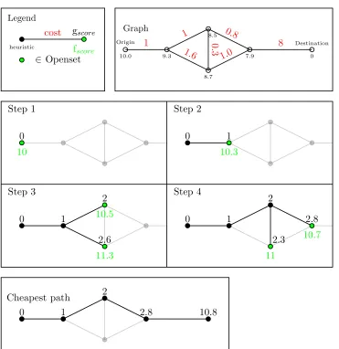
Figure 1: Example of functioning of A*
Step 1 Step 2
Step 3 Step 4
Legend cost
heuristic
gscore
fscore
∈ Openset
Graph
1 1
1.6
0.8
0.3
1.0
8
10.0 Origin
9.3
8.5
8.7
7.9 0
Destination
0
10
0 1
10.3
0 1
11.3 10.5
2
2.6
0 1
2
2.8
11
10.7
2.3
Cheapest path
0 1
2
5.3 Non-classical shortest-path problem
The main reason why A* does not guarantee an optimal path is that the costs per link are not CICO-consistent. This causes a problem for A*’s method of constructing a shortest-path tree.
The construction of this tree requires that a shortest path to a node n is also the start of the shortest path to all subsequent nodes in the tree. If the costs are CICO-consistent then that would be true, but the costs are not CICO-consistent. Therefore it is possible that there is a different path to node n which is a more expensive way to get to node n
but it results in a cheaper path to a subsequent node. The following example describes the situation where the construction of the tree in A* can loose the shortest path.
Example 5.1
We want to solve a SCP for freight demand d = (origin, destination, Trelease
d , Fd) with
A*. Let some path Pfrom the origin to some node nbe in the tree constructed by the A* algorithm. LetP’6=P be a different path from the origin to node n, which has an earlier arrival time at noden but is more expensive thenP.
Let the arrival of path P at node n be at time T and the arrival of P’ at node n at time
T’, T’< T. Let the travel cost from node n to the destination, when leaving at time T, be higher then when leaving at timeT’. This can be the case when a traffic jam occurs on a road link between node n and the destination at such a time that departure at time T
causes the freight shipmet to encounter the traffic jam, but the traffic jam will not yet be there when departure is done at timeT’.
In this situation it can happen that a path from the origin to the destination via node n
with path P’ is cheaper then travelling with path P. However node n was already in the tree of A* via path P, meaning that path P’ will not be found by A* and A* would not produce an optimal path.
In section 5.1.3 we stated that A* can be used to find the cheapest path on a single modality problem. In our setting of the SCP there are two main modalities: truck and barge. All freight originates at Rotterdam and also all barges have a departure at this location. This causes that the paths generally consist of only a path by truck or of first a path by barge and then a path by truck.
end of the virtual link to the destination is the optimal truck route and the virtual link is necessary to get out of the origin. It can also be that the resulting path is partly by barge and partly by truck. For all parts we can be sure that it is the cheapest path with the specific modality, but we cannot be sure that the entire path is the cheapest solution.
If it is not the cheapest then there must be some node in the tree constructed by A* where the cheapest path is lost. This can happen as described in Example 5.1 or a similar situation. These situations are quite specific, because the point of loosing the optimal path in the construction of the A* tree has at least the following two requirements. The first requirement is that there are branches in the tree which reach to the same node with different cost and different travel time. These differences leading to the loss of optimality can only be caused by branches using different modalities. The other requirement is that there must be a significant cost difference, thus a significant travel time difference between the node and the destination.
The first requirement can only be met by a limited amount of nodes where these branches using different modalities cross. The second requirement is not likely to be met at these nodes, because most destinations are in the hinterland where there is less traffic congestion, which would be the main cause of a significant travel time difference. These reasons create the situation of A* not finding an optimal path quite specific. Therefore we choose to use A* algorithm to find a cheap or even the cheapest path for SCP. To ensure that the resulting paths from the A* path do not differ to much from the cheapest paths a checking method was implemented. This method is described in the next section and it checks if a possible better path is lost during tree construction.
5.3.1 Check for suboptimality
To keep an eye on the possibility of the occurrance of A* finding a suboptimal path, checking algorithmA*Check was implemented.
First we take the following notation from the pseudocode of A*: gscore(n) denotes the
cost for travelling from origin to nodenvia the A* tree. gtime(n) denotes the travel time
of travelling to node n via the A* tree. For nodes a, b, time T and freight size F, let
cost(a, b, T, F) and time(a, b, T, F) represent the cost and the travel time for travelling from nodeato nodebwith departure time T and freight sizeF. These functions are part of the earlier mentioned functiontrans(a, b, gscore, T, F). In words the checking algorithm
does the following: Let Zd be the tree constructed by A* for d ∈ OD, for each node n
in Zd, for all neighbors of n check if a cheaper path could exist. Let x be a neighbor of n. A cheaper path can exist via x if ttime(x) +time(x, n, gtime(x), Fd) < ttime(n) and if gscore(x) < gscore(Dd). If both these conditions hold compare the costs of travelling via x
1. A*Check(Pd, Zd, gscore, ttime)
2. ∀n∈Zd, ∀a∈Ainn, a= (i, n)
3. If ttime(i) +time(i, n, ttime(i), Fd)< ttime(n) and
4. gscore(i)< gscore(Desd)
then do
5. cost(i, Desd, ttime(i), Fd):=A* {i, Desd, ttime(i), Fd}, G(N, A)
6. If gscore(i) +cost(i, Desd, ttime(i), Fd)≤gscore(Desd) then do
7. gˆ(i) =gscore(i) +cost(i, Desd, ttime(i), Fd)
8. end
9. end
10. return(ˆg)
In the verification section in Chapter 6 we show that this algorithm can find path improvements on paths resulting from the A* algorithm. This result gives us an indication in the difference between the paths resulting from A* and the possible cheaper paths. In the following section we take a look at the other issue that makes SCP a non-classical shortest-path problem, which is the waiting time at terminals.
5.4 Waiting-time expansion
In the model in Chapter 4 a variable was integrated to represent waiting time at a terminal. The A* algorithm is not able let a freight shipment wait at a terminal. This section describes a method to make A* find a path including waiting times.
To incorporate the variable waiting time at a terminal, the idea of time expansion is used. The idea of a Time-Expanded network is described in section 3.2.4. Instead of doing an expansion of the entire network only expansion is done on the tree made by A*. The algorithm is modified such that the tree can have several branches to the same node in different time expansions. Each time expansion represents a period of waiting time at a terminal. This allows a single node to occur on several places in the cheapest path tree. The different branches to that same node indicate a path with a different number of waiting time periods at specific terminals.
A* adds a nodento the tree if it has the lowest possible score of a set of reachable nodes. The neighbours of this node n will then be added to the set of reachable nodes. If it is possible to wait at a terminal, then for each waiting period the neighbor node, with a time expansion index, is added to the set of reachable nodes. Then in the next step it is possible that a time expansion indexed node is added to the shortest-path tree. Finally when A* reaches the goal node it is possible that the constructed path includes a waiting period at a terminal.
Pseudocode of the time-expansion method
Let expansion number be the possible number of waiting periods at a terminal and let
maxexpbe a predefined maximum number of expansions for each branch of the tree. The pseudocode of the method is added to the peudocode of A*, the line numbers originate from the same pseudocode in section 5.2.2.
7. {currentnode, currentexp}:= argminn∈Openset,exp∈[1,maxexp]fscore[n, exp]
12. For neighbour∈Neighbours[currentnode]do
For expand ∈[1 toexpansion number]do
exp=currentexp+expand
If exp≤maxexpdo
13. {gˆscore,tˆtime}:=trans currentnode, neighbour,gscore,ttime,f reight,exp
14. If neighbour /∈Openset orgˆscore <gscore[neighbour, exp]then do
15. gscore[neighbour, exp] = ˆgscore
16. ttime[neighbour, exp] = ˆttime
17. fscore[neighbour, exp] = ˆgscore+heur(currentnode, goalnode, f reight)
18. came f rom[neighbour, exp] ={currentnode, currentexp}
19. make sureneighbour is in Openset
20. end
Elsego to next neighbour
end
21. end
5.5 ICPA*
In the previous section the approach of solving the SCP with waiting at terminals and the possibility of A* not finding an optimal path is described. However, our main goal is to solve the ICP to find a solution to the DTA problem.
As described in Chapter 4 we do this by iteratively solving SCP and in between the iterations add the load resulting from the solution of SCP onto the network. This means that after each iteration some available capacity of the network is claimed. It remains to determine the order in which to solve the SCP, this will be discussed furtheron in this section. First we give pseudocode of the used ICP solving algorithm, this algorithm will be called ICPA*. For this, let σ define the order in which the SCP will be solved. The functionLoaddefines the capacities that are required for path Pdwith freightFd; the load
that is required for the network update.
5.5.1 Pseudocode of ICPA*
1. ICPA* G(N, A), OD, σ)
2. For d∈σ(OD) do
3. Pd:=A* {Od, Dd, Tdrelease, Fd}, G(N, A)
4. Update network: G(N, A) =G(N, A) +Load(Pd, Fd)
5. end
6. return(P)
5.5.2 Order of assigning
Note that there are limited capacities in the ICP. Updating these capacities after assigning freight shipments causes that later assigned shipments cannot use this capacity. This means that earlier solved SCP can choose from more feasible paths and can choose the cheapest feasible paths. Therefore, the order of assigningσinfluences the cost for individual shipments and therefore also the total cost. Thus different orders of iteration can result in a different total cost.
6
Implementation
This section deals with the implementation of the ICPA* algorithm in TransCAD and its verification. Next to analyzing if the algorithm does what it should, calibration of parameters is done. No validation of results will be done as not enough data is available to do a significant validation.
6.1 TransCAD
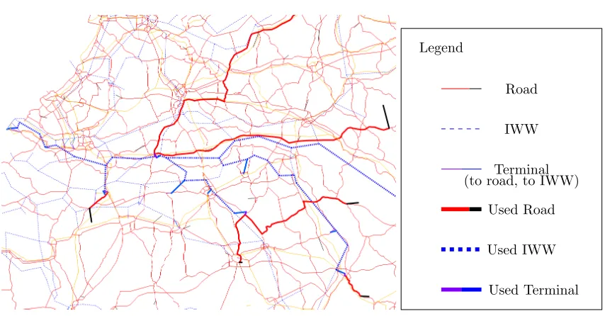
[image:39.612.91.518.355.578.2]The ICPA* algorithm has been implemented in the developers environment of TransCAD. TransCAD is created by the Caliper Cooperation. It is an extensive software system that can be used for all kinds of transportation problems. TransCAD supports transportation and route optimization models and includes tools for creating and displaying traffic networks. An example of a route map in TransCAD can be seen in Figure 2. Next to the implemented functions and tools it is possible to create macros in the Geographic Informations System Developer’s Kit(GISDK). With these macros it is possible to program algorithms that use the network structures, network data and tools of TransCAD.
Figure 2: Example of TransCAD routemap
Legend
Road
IWW
Terminal (to road, to IWW)
Used Road
Used IWW
6.2 ICPA* implementation
For the implementation of the ICPA* algorithm we first define the setting and requirements. For the A* algorithm we need a network, the barges, the heuristic function and the costs per link. The costs per link are time and modality dependent and the calculation of the travel time for the different modalities is also discussed. Next to this setting for the A* algorithm we also require freight demand requests to assign to the network.
6.2.1 Freight demand
A setODwith all freight requests is required. No real freight traffic information is available, but a setODcan be randomly generated. A random generator is developed by Zhang [38] and was made to create a set of freight demand that represents a day of container freight originating from Rotterdam. The random generation is based upon data from Panteia and TNO [26].
The generator creates a realistic day of freight demand if the created set has a size around 1000 freight demand requests. It is also possible to use the random generator to create a smaller OD set with less requests. Such a smaller set will be used for the verification and calibration. For each individuald∈OD a cheap path will be generated with the A* algorithm.
6.2.2 A* implementation
For the implementation of the A* algorithm we need to define the heuristic function and the cost function. Pseudocode of the A* algorithm can be found in section 5.2.2.
The heuristic function
In the pseudocode of A* we mentioned the function heur(startnode, goalnode, f reight). This function needs to make an estimation for the costs of transporting f reight from a
startnodeto a goalnode, but it should not overestimate the real costs.
The estimation is therefore based upon the costs of a cheapest path in a static situation. Determining these costs for a static situation can be done faster than for a the dynamic situation. We choose the following safe and fast method to ensure that the estimation is not higher than the real costs.
are minimal and therefore the time related costs are never overestimated by this heuristic. Note that this shortest-path function of TransCAD does not take into account vehicles or capacities, this implies that there are no transfer costs or waiting costs in the estimation. .
Costs per link
Another requirement for using A* is defining the weights per link, where the weights represents the costs. From Chapter 5 we have the following cost function (11) for defining a cost per linka.
Ca(td,a, twaitd,a , Fd, T) =Fd
td,a(T)cta+twaitd,a ct,waita
,
The value of the different cost factors can be found in the next paragraph. How the travel times are determined is explained furtheron in this section.
Costs of transport
Costs of the different transport modalities and other transport costs per minute can be found in Table 1 below. The costs are gained from several reports on freight transport in the Netherlands [25] [30] [31]. Costs for loading and unloading a barge is around e33 per TEU [25]. A loading time of 3 minutes per TEU results in a cost of e11 per minute for handling a TEU. Note that Table 1 contains a containercost cd, this time related cost
[image:41.612.186.432.456.545.2]represents the costs of renting shipping container. This cost makes every minute of travel or waiting from origin to destination more expensive.
Table 1: Costs in Euro per TEU per minute for the different transportation modalities.
Specification Notation Euro/(TEU·minute) Truck cta, a∈R e0.86 Barge ship cta, a∈W e0.015 Waiting cost ct,waita ,∀a e0.005
Handling cost cta, a∈V e11 Container cost cd e0.055
6.2.3 The network