Learning semantic features for fMRI data from definitional text

Learning semantic features for fMRI data from definitional text

Francisco Pereira, Matthew Botvinick and Greg Detre

Psychology Department and Princeton Neuroscience Institute Princeton University

Princeton, NJ 08540

{fpereira,matthewb,gdetre}@princeton.edu

Abstract

(Mitchell et al., 2008) showed that it was pos-sible to use a text corpus to learn the value of hypothesized semantic features characterizing the meaning of a concrete noun. The authors also demonstrated that those features could be used to decompose the spatial pattern of fMRI-measured brain activation in response to a stimulus containing that noun and a picture of it. In this paper we introduce a method for learning such semantic features automatically from a text corpus, without needing to hypoth-esize them or provide any proxies for their presence on the text. We show that those fea-tures are effective in a more demanding classi-fication task than that in (Mitchell et al., 2008) and describe their qualitative relationship to the features proposed in that paper.

1 Introduction

In the last few years there has been a gradual in-crease in the number of papers that resort to machine learning classifiers to decode information from the pattern of activation of activation of voxels across the brain (see (Norman et al., 2006) and (Haynes and Rees, 2006) for pointers to much of this work). Re-cently, however, interest has shifted to discovering how the information present is encoded, rather than just whether it is present, and also testing theories about that encoding. One especially compelling ex-ample of the latter is (Kay et al., 2008), where the authors postulate a mathematical model for how vi-sual information gets transformed into the fMRI sig-nal one can record from visual cortex and, after fit-ting the model, validate it by using it to predict fMRI

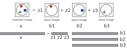
Figure 1: top: A complex pattern of activation is

ex-pressed as a combination of three basic patterns.bottom:

The pattern can be written as a row vector, and the com-bination as a linear comcom-bination of three row vectors.

activation for novel stimuli. A second example is, of course, (Mitchell et al., 2008), which aims at de-composing the pattern of activation in response to a picture+noun stimulus into a combination of basic patterns corresponding to the key semantic features of the stimulus. A schematic view of this is given in Figure 1, where the complex pattern on the left is split into three simpler ones. This is done by deter-mining the value of several hypothesized semantic features and using them as the combination weights for basic patterns, which can then be extracted from fMRI data.

Ideally, semantic features should reflect what is in a subject’s mind when she thinks about a con-crete concept, e.g. whether it is animate or inani-mate, or an object versus something natural. It also seems reasonable to expect that the main seman-tic features would likely be shared by most people thinking about the same concept; talking to some-one about a chair or table requires a common un-derstanding of the characteristics of that concept. (Mitchell et al., 2008) proposed a method for captur-ing such common understandcaptur-ing, by considercaptur-ing 25

verbs1reflecting, in their words, “basic sensory and motor activities, actions performed on objects, and actions involving changes to spatial relationships”. For each of the 60 nouns corresponding to the stim-ului shown, they counted the co-occurrence of the noun with each of the 25 verbs in a large text corpus, converting those 25 counts into normalized feature values (the 25-vector has length 1). The hypothe-sis subjacent to this procedure is that the 25 verbs are a good proxy for the main characteristics of a concept, and that their frequent co-occurrence with the corresponding noun in text means that many dif-ferent sources (and people) have that association in mind when using the noun; in a nutshell, the associa-tion reflects common understanding of the meaning of the noun. The results in (Mitchell et al., 2008) are an extremely compelling demonstration that text corpora contain information useful for parsing brain activation into component patterns that reflect se-mantic features.

We would like to go beyond the analysis in (Mitchell et al., 2008) by considering that stipulat-ing the semantic features to consider – via the verb proxy – may limit the information that can be ex-tracted. The verbs were selected to capture a range of characteristics described above, but this does not guarantee that those will be all the ones that are rele-vant, even for concrete concepts. But how to identify characteristics beyond those that one could hypoth-esize in advance?

This paper describes an approach to identifying semantic features from a text corpus in an unsuper-vised manner, without the need to specify verbs or any other proxy for those features. The first aspect of the approach is the use of a text corpus that goes beyond merely containing occurrences of the words. We use a subset of Wikipedia2, which we chose be-cause articles are definitional in style and also edited by many people, ensuring that they will contain the essential shared knowledge pertaining to the subject of the article. The articles in the subset were cho-sen because they pertained to concrete or imageable concepts, and the methodology for deciding on this is described in Section 2.2.2. One property in

par-1_{see, hear, listen, taste, smell, eat, touch, rub, lift,}

manipu-late, run, push, fill, move, ride, say, fear, open, approach, near, enter, drive, wear, break and clean

2

http://en.wikipedia.org

ticular of text defining a concept will be especially helpful here: in order to make its meaning precise, it has to touch on most related concepts. This means that we will still be resorting to co-ocurrence with our target nouns in order to identify semantic fea-tures, but not of a fixed set of verbs; rather, we are considering all possible related words.

The tool we will use to do so is latent Dirichlet allocation (LDA, (Blei et al., 2003)). This tech-nique produces a generative probabilistic model of text corpora where each document (article) is viewed as a bag-of-words (i.e. only which words appear, and how often, matters) with each word being drawn from a finite mixture of an underlying set oftopics, each of which is in turn a probability distribution over vocabulary words. We will use topics as our semantic features, with the proportions of each topic in the article for a given noun being the values of the features for that noun.

(Murphy et al., 2009) does something similar in flavour to this, by decomposing the patterns of co-occurrences in a text corpus between the 20000 most frequent nouns and 5000 most frequent verbs using SVD. This is used to identify 25 singular vectors which yield feature values across nouns.

2 Methods and Data

2.1 Data

We use the dataset from (Mitchell et al., 2008), which contains data from 9 subjects. For each sub-ject there is a dataset of 360 examples - average fMRI volume around the peak of an experiment trial - comprising 6 replications (epochs) of each of 60 nouns as stimuli. The 60 nouns also belong to one of 12 semantic categories, hence there are two la-bels for classification tasks. We refer the reader to the original paper for more details about the specific categories and nouns chosen.

2.2 Semantic Features

The experiments described on the paper rely on us-ing two different kinds of semantic features (low-dimensional representations of data) to decompose each example in constituent basis images; these two kinds are described blow.

2.2.1 Science Semantic Features (SSF)

These are the semantic features used in (Mitchell et al., 2008) to represent a given stimulus. They were obtained by considering co-occurrence counts of the noun naming each stimulus with each of 25 verbs in a text corpus, yielding a vector of 25 counts which was normalized to have unit length. The low-dimensional representation of the brain image for a given noun is thus a 25-dimensional vector. The left of Figure 2 shows the value of these features for the 60 nouns considered.

2.2.2 Wikipedia Semantic Features (WSF)

To obtain the Wikipedia semantic features we considered concepts rather than nouns, though we will use the latter terminology in the rest of the pa-per for consistency with (Mitchell et al., 2008). We started with the classical lists of words in (Paivio et al., 1968) and (Battig and Montague, 1969), as well as modern revisions/extensions (Clark and Paivio, 2004) and (Van Overschelde, 2004), and looked for words corresponding to concepts that were deemed concrete or imageable (be it because of their score in one of the norms or through editorial decision), identified the corresponding Wikipedia article ti-tles (e.g. “airplane” is “Fixed-wing aircraft”) and also compiled related articles which were linked to from these (e.g. “Aircraft cabin”). If there were words in the original lists with multiple mean-ings we included the articles for at least several of those meanings. Given the time available, we stopped the process with a list of 3500 concepts and their corresponding articles (a corpus we call the “Weekipedia”). We used Wikipedia Extractor 3 to remove any HTML or wiki formatting and annota-tions and processed the resulting text through the morphological analysis tool Morpha (Minnen et al.,

3

http://medialab.di.unipi.it/wiki/ Wikipedia_extractor

2001) 4 to lemmatize all the words to their basic stems (e.g. “taste”,”tasted”,”taster” and “tastes” all become the same word).

The resulting text corpus was processed with topic modelling software to build several LDA mod-els. The articles were converted to the required for-mat, keeping only words that appeared in at least two articles, and words were also excluded resorting to a custom stopword list. We run the software vary-ing the number of topics allowed from 10 to 60, in increments of 5, and allowing the software to esti-mate theα parameter. The α parameter influences the number of topics used for each example. For a given number of topicsK, this yielded distributions over the vocabulary for each topic and one vector of topic probabilities per article/concept; this vector is the low-dimensional representation of the concept. Note also that, since the probabilities add up to 1, the presence of one semantic feature trades off with the presence of the others.

The middle and right of Figure 2 shows the value of these features for the 60 nouns considered in 25 and 50 topic models, respectively.

2.2.3 Relating semantic features to brain

images

notation Each example corresponds to the average

fMRI volume around the peak of a trial, account-ing for haemodynamic delay. This 3D volume can be unfolded into a vectorx_{with as many entries as}

voxels. A dataset is an×m matrixX where row i is the example vector x_{i. Similarly to (Mitchell}

et al., 2008), each examplex _{will be expressed as}

a linear combination of basis images b

1, . . . ,bK

of the same dimensionality, with the weights given by the semantic feature vector z _{= [z}

1, . . . , zK]

(see Figure 1 for an illustration of this). The low-dimensional representation ofX is an×Kmatrix Zwhere rowiis a semantic feature vectorz_{iand the}

corresponding basis images are aK×mmatrixB, where rowkcorresponds to basis imageb_k.

learning and prediction Learning the basis

im-ages givenXandZ(top part of Figure 4) can be de-composed into a set of independent regression

prob-4

Figure 2: The value of semantic features for the 60 nouns considered, using SSF with 25 verbs (left) and WSF with 25 and 50 topics (middle and right). The 60 nouns belong to one of 12 categories, and those are arranged in sequence. Although a few of the SSF features might correspond to WSF features, the majority of them do not.

lems, one per voxel j, i.e. the values of voxel j across all examples, X(:, j), are predicted from Z using regression coefficients B(:, j), which are the values of voxeljacross basis images.

Predicting the semantic feature vectorz_{for an}

ex-ample x _{(bottom part of Figure 4) is a regression}

problem wherex′_{is predicted fromB}′_using

regres-sion coefficientsz′_{. For WSF, the prediction of the}

semantic feature vector is done under the additional constraint that the values need to add up to 1. Any situation where linear regression was unfeasible be-cause the square matrix in the normal equations was not invertible was addressed by replacing the design matrix by its singular value decomposition, leaving only non-zero singular values.

3 Experiments and Discussion

3.1 Classification/Reconstruction on semantic

feature space

3.1.1 Experiment details

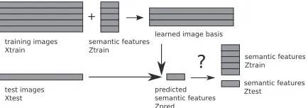
Several classification experiments are described in (Mitchell et al., 2008). The main one aims at gauging the accuracy of matching unseen stimuli to their unseen fMRI images and is schematized in Fig-ure 3. To do this, the authors consider the 60 average examples of each stimulus and, in turn, leave out each of 1770 possible pairs of examples. For each left out pair, they learn a set of basis images using the remaining 58 examples and their respective SSF representations. They then use the SSF

Figure 3: The classification task in (Mitchell et al., 2008) is such that semantic feature representations of the 2 test nouns are used, in conjunction with the image ba-sis learned on the training set, to predict their respective test examples and use that prediction in a 2-way classifi-cation.

tion of the two left-out examples and the basis to generate apredicted examplefor each one of them. These can then be used in a two-way matching task with the actual examples that were left out, where the outcome is correct or incorrect. Note that this is not done over the entire brain but over a selection of 500 stable voxels, as determined by computing their reproducibility over the 58 examples in each leave-one-out fold. This criterion identifies voxels whose activation levels across the 58 nouns bear the same relationship to each other over epochs (mathemat-ically, the vector of activation levels across the 60 sorted nouns is highly correlated between epochs). We reproduced this experiment for the sake of com-parison and describe the results in Section 3.4.

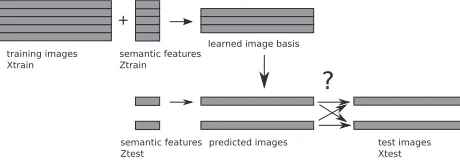
Figure 4: Our classification task requires learning an im-age basis from a set of training examples and their re-spective semantic feature representations. This is used to predict semantic feature values for test set examples and from those one can classify against the known semantic feature values for all 60 nouns.

good that prediction is by its 2-way accuracy, this paper focuses on a different sort of experiment: pre-diction of semantic feature values for a test exam-ple, as schematized in FIgure 4. In this experiment, the semantic features get used to learn basis images from training examples, with the goal of reconstruct-ing those trainreconstruct-ing examples as well as possible. This learning does not contemplate the labels – category or noun – of the training examples. The basis images are used, in turn, to predict semantic feature values for test examples and determining, in essence, which semantic features are active during a test example. The criterion for judging whether this is a good pre-diction will be how well can we classify the category (1-of-12) and noun (1-of-60) noun of a test example. Good classification performance implies that the se-mantic features capture activation that is relevant to the task in the corresponding basis images and that, in combination, the features contain enough infor-mation to distinguish the various nouns.

We will use either a leave-one-epoch-out (6 fold) or a leave-one-noun-out (60 fold) cross-validation and we perform the following steps in each fold:

1. from each training setXtrain and

correspond-ing semantic features Ztrain, select the top

1000 most reproducible voxels and learn an im-age basisB using those

2. use the test setXtest and basis B topredict a

semantic feature representationZpredfor those

examples

3. use nearest-neighbour classification to predict the labels of examples inXtest, by comparing

Zpred for each example with known semantic

featuresZ

4. use the semantic features Zpred together with

basis B to reconstruct test examples as Xpred = ZbredB and compute squared error

betweenXpredandXtest(over selected voxels)

This allows us to do both kinds of cross-validation, as there is always one semantic feature vector for each different noun inZ regardless. This procedure is unbiased, and we tested this empirically using a permutation test (examples permuted within epoch) to verify the accuracy results for either task were at chance level.

3.1.2 Experiment results

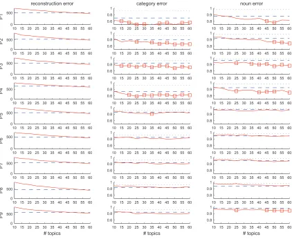
Figure 5 shows the results using leave-one-epoch-out cross-validation. For each subject (row), there is one plot of reconstruction error (column 1) and one for error in category classification (column 2) and noun classification (column 3). Each plot con-trasts the error obtained using SSF with that ob-tained using WSF with 10-60 topics, in increments of 5; WSF is as good or better than SSF in both cat-egory and noun classification. Given the the results are over 360 test examples we are not displaying er-ror bars; each number of topics for which WSF is better as deemed by a paired t-test (0.01 significance level, uncorrected) is highlighted by a square on the plot. The same is true for the category task when using leave-one-noun-out cross-validation, but nei-ther WSF nor SSF appear to do well in the noun task except for subject P1, where WSF again dom-inates. Results overall are somewhat lower than for the leave-one-epoch-out cross-validation. Given that the comparison results are qualitatively similar and space is limited we did not include the correspond-ing figure. In both cross-validations the reconstruc-tion error of WSF starts higher than that of SSF and decreases monotonically until they are roughly matched. Our conjecture is that WSF semantic fea-tures are sparser and thus there are fewer basis im-ages being added to predict any given test example. As the number of topics increases, this ceases to be the case.

10 15 20 25 30 35 40 45 50 55 60 0

500

reconstruction error

P1

10 15 20 25 30 35 40 45 50 55 60 0.6

0.8 1

category error

10 15 20 25 30 35 40 45 50 55 60 0.8

0.9 1

noun error

10 15 20 25 30 35 40 45 50 55 60 0

500

P2

10 15 20 25 30 35 40 45 50 55 60 0.6

0.8 1

10 15 20 25 30 35 40 45 50 55 60 0.8

0.9 1

10 15 20 25 30 35 40 45 50 55 60 0

500

P3

10 15 20 25 30 35 40 45 50 55 60 0.6

0.8 1

10 15 20 25 30 35 40 45 50 55 60 0.8

0.9 1

10 15 20 25 30 35 40 45 50 55 60 0

500

P4

10 15 20 25 30 35 40 45 50 55 60 0.6

0.8 1

10 15 20 25 30 35 40 45 50 55 60 0.8

0.9 1

10 15 20 25 30 35 40 45 50 55 60 0

500

P5

10 15 20 25 30 35 40 45 50 55 60 0.6

0.8 1

10 15 20 25 30 35 40 45 50 55 60 0.8

0.9 1

10 15 20 25 30 35 40 45 50 55 60 0

500

P6

10 15 20 25 30 35 40 45 50 55 60 0.6

0.8 1

10 15 20 25 30 35 40 45 50 55 60 0.8

0.9 1

10 15 20 25 30 35 40 45 50 55 60 0

500

P7

10 15 20 25 30 35 40 45 50 55 60 0.6

0.8 1

10 15 20 25 30 35 40 45 50 55 60 0.8

0.9 1

10 15 20 25 30 35 40 45 50 55 60 0

500

P8

10 15 20 25 30 35 40 45 50 55 60 0.6

0.8 1

10 15 20 25 30 35 40 45 50 55 60 0.8

0.9 1

10 15 20 25 30 35 40 45 50 55 60 0

500

# topics

P9

10 15 20 25 30 35 40 45 50 55 60 0.6

0.8 1

# topics

10 15 20 25 30 35 40 45 50 55 60 0.8

0.9 1

# topics

Figure 5: For each of the 9 subjects (rows) a comparison between SSF and WSF (using 10-60 topics) in reconstruction error (column 1) and classification error in the category (column 2) and noun (column 3) tasks. In each plot WSF is red (full line), SSF is blue (constant dashed line) and chance level is black (constant dotted line). The reconstruction error is measured on left out examples, over the 1000 voxels selected on the training set. These results were obtained using leave-one-epoch-out cross-validation (one epoch containing one instance of all nouns is left out in each of 6 folds). Error bars are not shown, given their small size (there are 360 examples), but each number of topics for which WSF error is significantly lower than SSF error is highlighted with a square.

P1 P2 P3 P4 P5 P6 P7 P8 P9

same 0.57 0.39 0.36 0.32 0.26 0.16 0.26 0.24 0.18 category 0.50 0.32 0.30 0.28 0.24 0.14 0.23 0.21 0.16 other 0.45 0.30 0.27 0.22 0.22 0.13 0.21 0.20 0.14

same minus other 0.12 0.09 0.09 0.10 0.04 0.03 0.05 0.04 0.04 same minus category 0.07 0.07 0.06 0.04 0.02 0.02 0.03 0.03 0.02

WSF is significantly better than SSF. In an effort to find out why this was the case, we computed a measure ofconsistencyof the data from each of the subjects; intuitively, this is the degree to which the brain activation pattern was similar between trials with the same noun stimulus (and dissimilar for tri-als where the stimulus was different). This was com-puted in leave-one-epoch-out cross-validation, and consisted of examining the correlation – computed across selected voxels – of a test example with train-ing examples of the same noun (same), the same category but a different noun (same category) and different category and noun (other); the measures were averaged across examples. In leave-one-group-out cross-validation subjects P1-P4 have higher dif-ferences between correlation within examples of a noun and examples in the same category or other categories than subjects P5-P9, which suggests that the former are more consistent in how they elicit pat-terns in response to the same stimulus.

3.2 Classification on voxel space

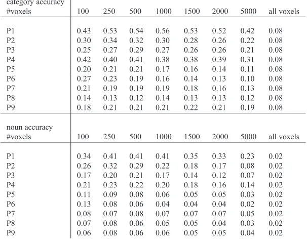
In order to have an idea of how much of the infor-mation present either SSF or WSF can extract and convey via their respective low-dimensional repre-sentations, we also trained a simple Gaussian Naive Bayes (GNB) classifier on voxels selected using the same reproducibility criterion described earlier. We used leave-one-epoch-out cross-validation and both category and noun tasks, respectively top and bot-tom of Table 2. Contrasting this with Figure 5, it’s clear that the accuracies in the category task are comparable, whereas those in the noun task are somewhat lower; this suggests that either informa-tion about individual nouns is lost when converting from voxels to semantic features, or that nearest-neighbour is not the best classifier to use.

3.3 Similarity between SSF and WSF

representations

In order to gauge the quality of the semantic feature representations we can consider both how much they differ between different nouns (and different cate-gories) and also how consistent they are for the 6 ex-amples of the same noun. This is shown for subject P1 in Figure 6, where the semantic feature vectors learned for 360 examples are correlated, for WSF 50 (left) and SSF 25 (right). Examples are sorted so that

WSF 50

SSF 25

correlation between 25 SSF and 50 WSF across 360 nouns

5 10 15 20 25 30 35 40 45 50

5

10

15

20

25

−1 −0.8 −0.6 −0.4 −0.2 0 0.2 0.4 0.6 0.8 1

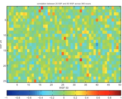
Figure 7: Correlation between each pair of SSF and WSF vectors of predicted feature values across 360 examples.

the 6 examples of the same noun are together, and adjacent to the other 24 belonging to the same cat-egory (and the catcat-egory changes are labelled. Note that these are the values obtained when each exam-ple was in the test set, rather than the values derived from text for each noun; this is why the semantic feature vectors for the 6 examples of the same noun are different. WSF 50 is such that nouns belonging to the same category share many feature values, and hence show up as large blocks along the diagonal of the correlation matrix. Less of the noun specific in-formation is being captured, but it is sometimes vis-ible as the smaller blocks along the diagonal, inside the large blocks.

We can also consider the question of whether SSF and WSF representations are similar, i.e. whether a given SSF feature has values across examples sim-ilar to a given WSF feature. This can be done by considering the correlation between each pair of predicted SSF/WSF vectors across 360 examples, which is shown in Figure 7. This suggests very few of the semantic features are similar when predicted for examples in the test set, and as was already evi-dence in Figure 2.

3.4 Leave-2-out 2-way classification

category accuracy

#voxels 100 250 500 1000 1500 2000 5000 all voxels

P1 0.43 0.53 0.54 0.56 0.53 0.52 0.42 0.08 P2 0.30 0.34 0.32 0.30 0.28 0.26 0.22 0.08 P3 0.25 0.27 0.29 0.27 0.26 0.26 0.21 0.08 P4 0.42 0.40 0.41 0.38 0.38 0.39 0.31 0.08 P5 0.20 0.21 0.21 0.17 0.16 0.14 0.11 0.08 P6 0.27 0.23 0.19 0.16 0.14 0.13 0.10 0.08 P7 0.21 0.19 0.19 0.19 0.18 0.16 0.13 0.08 P8 0.14 0.13 0.12 0.14 0.13 0.13 0.12 0.08 P9 0.18 0.21 0.21 0.21 0.22 0.21 0.19 0.08

noun accuracy

#voxels 100 250 500 1000 1500 2000 5000 all voxels

P1 0.34 0.41 0.41 0.41 0.35 0.33 0.23 0.02 P2 0.26 0.32 0.29 0.22 0.18 0.17 0.08 0.02 P3 0.17 0.20 0.21 0.17 0.14 0.12 0.07 0.02 P4 0.21 0.23 0.22 0.20 0.18 0.16 0.14 0.02 P5 0.11 0.09 0.08 0.06 0.05 0.05 0.03 0.02 P6 0.13 0.08 0.06 0.04 0.04 0.04 0.02 0.02 P7 0.08 0.07 0.08 0.07 0.07 0.07 0.05 0.02 P8 0.07 0.08 0.06 0.05 0.05 0.04 0.03 0.02 P9 0.06 0.08 0.06 0.06 0.05 0.05 0.04 0.02

Table 2: top: Accuracy of a Gaussian Naive Bayes classifier trained on various numbers of voxels selected by the

reproducibility criterion, on the category prediction task, using leave-one-epoch-out cross-validation.bottom:Same,

for the noun prediction task.

animal (1)

bodypart (31) building (61)

buildingpart (91)

clothing (121) furniture (151) insect (181) _{kitchen (211)}

manmade (241)

tool (271)

vegetable (301)

vehicle (331)

correlation between predicted WSF 50 dimensional vectors for 360 nouns animal (1)

bodypart (31) building (61) buildingpart (91) clothing (121) furniture (151)

insect (181) kitchen (211) manmade (241) tool (271) vegetable (301) vehicle (331)

0 0.2 0.4 0.6 0.8 1

animal (1)

bodypart (31) building (61)

buildingpart (91)

clothing (121) _{furniture (151)} insect (181) kitchen (211)

manmade (241)

tool (271)

vegetable (301)

vehicle (331)

correlation between predicted SSF 25 dimensional vectors for 360 nouns animal (1)

bodypart (31) building (61) buildingpart (91) clothing (121) furniture (151) insect (181) kitchen (211) manmade (241) tool (271) vegetable (301) vehicle (331)

0 0.2 0.4 0.6 0.8 1

Figure 6: left: correlation between the WSF 50 predicted feature vectors for the 360 examplesright: same for the

SSF Org 20 25 30 35 40 45 50

P1 0.84 0.83 0.88 0.91 0.87 0.89 0.85 0.85 0.86

P2 0.80 0.76 0.75 0.77 0.74 0.76 0.72 0.72 0.73

P3 0.78 0.78 0.76 0.78 0.73 0.76 0.72 0.70 0.78

P4 0.82 0.72 0.88 0.88 0.85 0.86 0.86 0.85 0.87

P5 0.85 0.78 0.79 0.84 0.78 0.71 0.78 0.73 0.78

P6 0.77 0.85 0.82 0.84 0.78 0.79 0.76 0.81 0.75

P7 0.78 0.73 0.83 0.84 0.80 0.81 0.79 0.75 0.74

P8 0.77 0.68 0.66 0.68 0.64 0.62 0.67 0.64 0.69

P9 0.75 0.82 0.77 0.81 0.77 0.79 0.81 0.78 0.78

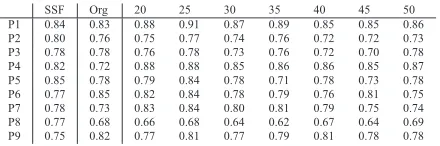
Table 3: Results of a replication of the leave-2-noun-out 2-way classification experiment in (Mitchell et al., 2008). For subjects P1-P9, SSF represents the mean accuracy obtained using SSF (across 1770 leave-2-out pairs), Org the mean accuracy reported in (Mitchell et al., 2008) and the remaining columns the mean accuracy obtained using WSF with 20-50 topics.

1770 leave-2-out pairs using SSF, the mean accuracy reported in (Mitchell et al., 2008) and the mean ac-curacy using WSF with 20-50 topics. We were not able to exactly reproduce the numbers in (Mitchell et al., 2008), despite the same data preprocessing (making each example mean 0 and standard devia-tion 1, prior to averaging all the repetidevia-tions of each noun, and then subtracting the mean of all average examples from each one), the same voxel selection procedure (using 500 voxels) and the same ridge re-gression function (although (Mitchell et al., 2008) does not mention the value of the ridge parameterλ, which we assumed to be 1). We will endeavour to identify the source of the discrepancies, but it was not possible to do so in time for this paper.

4 Conclusions

We have shown that it is feasible to learn seman-tic features from a text corpus, without the need to postulate what they might represent in the brain, ei-ther directly or via proxy indicators like the verbs in (Mitchell et al., 2008). Furthermore, we have shown that those semantic features are superior to the fea-tures proposed in (Mitchell et al., 2008) in two de-manding classification tasks that require using the features to decompose brain activation into basis im-ages related to them. Further analysis of those and other results obtained classifying directly from vox-els suggest that the semantic features capture a large amount of category-level information, and at least a fraction of the noun-level information present in the pattern of brain activation. (Mitchell et al., 2008).

Acknowledgments

We would like to thank David Blei for discussions about topic mod-elling in general and of the Wikipedia corpus in particular and Ken Norman for valuable feedback at various stages of the work.

References

William F Battig and William E Montague. 1969.

Cate-gory Norms for Verbal Items in 56 Categories. Journal

of Experimental Psychology, 80(3).

D M Blei, A Y Ng, and M I Jordan. 2003. Latent

Dirich-let allocation. Journal of Machine Learning Research,

3:993–1022.

James M Clark and Allan Paivio. 2004. Extensions of

the Paivio, Yuille, and Madigan (1968) norms.

Be-havior research methods, instruments, & computers : a journal of the Psychonomic Society, Inc, 36(3):371– 83, August.

John-Dylan Haynes and Geraint Rees. 2006. Decoding

mental states from brain activity in humans. Nature

reviews. Neuroscience, 7(7):523–34.

Kendrick N Kay, Thomas Naselaris, Ryan J Prenger, and Jack L Gallant. 2008. Identifying natural images from

human brain activity. Nature, 452(7185):352–5.

G. Minnen, J. Carroll, and D. Pearce. 2001. Applied

morphological processing of English. Natural

Lan-guage Engineering, 7(03):207223.

Tom M Mitchell, Svetlana V Shinkareva, Andrew Carl-son, Kai-Min Chang, Vicente L Malave, Robert a Ma-son, and Marcel Adam Just. 2008. Predicting human brain activity associated with the meanings of nouns. Science (New York, N.Y.), 320(5880):1191–5.

B. Murphy, M. Baroni, and M. Poesio. 2009. EEG Re-sponds to Conceptual Stimuli and Corpus Semantics. Proceedings of ACL/EMNLP.

Kenneth A Norman, Sean M Polyn, Greg J Detre, and James V Haxby. 2006. Beyond mind-reading:

multi-voxel pattern analysis of fMRI data. Trends in

cogni-tive sciences, 10(9):424–30.

Allan Paivio, John C Yuille, and Stephen A Madigan.

1968. Concreteness, Imagery, and Meaningfulness

Values for 925 Nouns. Journal of Experimental

Psy-chology, 76(1).

J Van Overschelde. 2004. Category norms: An

up-dated and expanded version of the Battig and

Mon-tague (1969) norms. Journal of Memory and