Learning Feed-Forward Control with the
Python Scikit-Learn Library
E.A. (Elise-Ann) Schrijvers
MSc Report
C
e
Dr.ir. J.F. Broenink
Dr.ir. T.J.A. de Vries
Dr.ir. G.M. Bonnema
October 2017
045RAM2017
Robotics and Mechatronics
EE-Math-CS
University of Twente
iii
Summary
The research of this thesis is about using a learning feed-forward controlled system in a plat-form independent way. To achieve this, the feed-forward part of the control system is imple-mented in Python while the general control system is within the 20-sim simulation environ-ment. The implementation of LFFC in Python is relatively simple due to the existence of the Scikit-learn library. This library enables the use of a B-spline network (function approximator).
Communication between both environments is achieved by setting up a network connection. To that end, data will be serialized and packed by the Protocol Buffer library from Google and ZeroMQ. The data can now be sent over the network in a proper and structured way.
The 1-dimensional time-indexed LFFC is implemented twice. One is completely built-up in the environment of 20-sim and the other has its feed-forward part built-up in Python. A 1-dimensional state-indexed LFFC in Python is considered as well. All implementations are demonstrated by assuming an ideal linear motor model (moving mass) representing the plant of the control system.
Contents
Summary iii
1 Introduction 1
1.1 Context . . . 1
1.2 Problem Statement . . . 1
1.3 Thesis Outline . . . 2
2 Theoretical Background 3 2.1 Learning Feed-Forward Control . . . 3
2.2 Function Approximation with B-splines . . . 5
2.2.1 B-spline Basis Functions . . . 8
2.2.2 Computing Coefficients . . . 11
2.3 B-spline Network Tools . . . 11
2.3.1 B-spline Network with 20-sim B-spline Editor . . . 11
2.3.2 B-spline Network with Python Scikit Learn Library . . . 13
2.4 Illustrative Application: Linear Motor Motion System . . . 14
2.4.1 Introduction to a Linear Motor . . . 14
2.4.2 Design of Linear Motor Model . . . 16
2.4.3 Design of Feedback Controller . . . 16
2.4.4 Performance Check on the Feedback System Model . . . 17
3 Network Communication 19 3.1 Introduction . . . 19
3.2 Design of Network Layer . . . 19
3.3 Implementation of Network Layer . . . 20
3.3.1 ZeroMQ . . . 20
3.3.2 Protocol Buffer from Google . . . 21
3.3.3 Network Communication with 20-sim . . . 22
3.4 Validation of Network Layer . . . 23
3.4.1 ZeroMQ Test . . . 23
3.4.2 Data Transfer Test . . . 24
3.5 Conclusion . . . 25
4 One Dimensional LFFC 26 4.1 Time-Indexed LFFC . . . 26
4.1.1 Design . . . 26
CONTENTS v
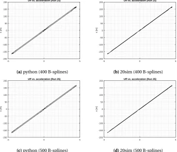
4.1.3 Comparison 20-sim and Python . . . 32
4.1.4 Conclusion . . . 41
4.2 State-Indexed LFFC . . . 42
4.2.1 Design . . . 42
4.2.2 Implementation . . . 43
4.2.3 Simulations . . . 50
4.2.4 Conclusion . . . 52
5 Two Dimensional LFFC 53 5.1 Parsimonious LFFC . . . 53
5.1.1 Design . . . 54
5.1.2 Implementation . . . 57
5.1.3 Simulations . . . 58
5.1.4 Conclusion . . . 61
5.2 Multidimensional BSN . . . 62
5.2.1 Design . . . 62
5.2.2 Implementation . . . 64
6 Conclusion 65 6.1 Conclusion . . . 65
6.2 Future Work . . . 65
A Partial Cubic Motion Profile (20-sim) 67 B More about B-splines 68 B.1 Properties of B-spline Basis Functions . . . 68
B.2 Properties of B-spline Curves . . . 68
B.2.1 Moving Control Points . . . 70
B.2.2 Modifying Knots . . . 71
C Implementation details (1D state-indexed LFFC) 72
D Implementation details (2D state-indexed LFFC) 75
Nomenclature
1D 1-dimensional
2D 2-Dimensional
ANOVA ANalysis Of VAriance
BSN B-Spline Network
CA Constant Acceleration
CV Constant Velocity
CY Constant Jerk
DLL Dynamic Link Library
FA Function Approximation
LC Learning Controller
LFFC Learning-Feed Forward Control
LMMS Linear Motor Motion System
NM No Movement
1
1 Introduction
1.1 Context
Learning Feed-Forward Control (LFFC) has proven to be a powerful control architecture that has much potential for control of mechatronic systems, Velthuis (2000). A LFFC system con-sists of a model-based feedback component and a feed-forward component that has learning abilities, i.e. it consists of a function approximator. The feedback part is a typical PD-type controller.
Starrenburg et al. (1996) started studying LFFC and later also Velthuis (2000) using B-spline Net-works (BSN) on repetitive motions. He performed a stability analysis on the LFFC and came up with rules to be able to properly select design parameters for such type of motions. Besides the LFFC for repetitive motions he also study non-repetitive motions. In this part he addressed multi-dimensional B-spline networks and introduced parsimonious LFFC. The latter was a so-lution to overcome the problems that go along with the curse of dimensionality. He used among others a linear motor motion system (LMMS) as an illustrative example for his study. The study from Velthuis (2000) is used as the base for this thesis.
1.2 Problem Statement
Simulations are commonly done in a Windows environment, for which real-time aspects are not so important, while experiments are done in a real-time Linux environment. This assign-ment addresses to find a solution to interact between the feed-forward part of a control system and a general PD-controlled system in a platform independent way. Therefor a network con-nection has to be incorporated into the control system.
The problem encounters to create and application that:
• is as straight forward as possible while at the same time the LFFC features (high perfor-mance and high robustness) are still maintained
• overcomes the following drawbacks that appear in currently available applications:
1. the computational intensiveness of the learning process 2. impossibility to combine LFFC with real-time control
3. restricted use in the type of function approximator that can be used (BSN). A BSN might not always result in the optimal combination with LFFC
4. testing the LFFC and painlessly transfer to a realization environment is not that simple
The envisioned solution is:
• to use Python Scikit-learn for the learning process (function approximation (FA)), as it provides BSN and other FA’s and it is platform independent. Unfortunately, this library is not directly suitable for real-time applications.
• to connect to Python via a network, such that this can be done both in simulation and in practice. But also to do learning at another computer than real-time control.
• to demonstrate LFFC in the simulation environment of 20-sim, followed by separating the feed-forward controlled part from the simulation environment and implement it in Python.
1.3 Thesis Outline
In Chapter 2 some background is provided about learning feed-forward control and how func-tion approximafunc-tion is performed using B-splines. An introducfunc-tion is given about implement-ing B-spline networks in the environments of 20-sim and Python. The background chapter is concluded with describing the illustrative example used for the thesis: a linear motor motion system.
In Chapter 3 the network communication set-up between 20-sim and Python is explained. Two protocols are discussed that perform data packaging and the data transfer between both ends of the communication network (Protocol Buffer from Google and ZeroMQ). The chapter is con-cluded with tests that will verify if both protocols work individually, but also if both protocols perform correctly when both are combined.
Chapter 4 demonstrates the use of 1-dimensional LFFCs. First a time-indexed LFFC is dis-cussed implemented in the environments of 20-sim and Python. The second part of the chap-ter demonstrates the use of 1-dimensional state-indexed LFFC in Python.
A 2-dimensional LFFC is discussed in Chapter 5. This chapter distinguishes between the use of two 1-dimensional B-spline networks (parsimonious LFFC) and one 2-dimensional BSN. The latter is only briefly discussed and is not demonstrated with simulations. More research is required about this topic.
3
2 Theoretical Background
This chapter provides the reader from information in order to understand the subjects treated in the thesis. The information starts with explaining what learning feed-forward control (LFFC) is and why it is used. Depending on the inputs of the feed-forward part a time-indexed or state-indexed LFFC is preferred, both types are treated.
An important part of LFFC is the function approximator, although there are many possible types of function approximators only the B-spline network (BSN), de Kruif and de Vries (2000) will be treated as this is the method used in the thesis.
Two different BSN implementations will be discussed, one describes the implementation using the built-in B-spline editor from the simulation software 20-sim and the other describes the implementation using the Scikit-learn library from Python.
In the last section an illustrative example is given. The example used is a plant that represents a model of a linear motor motion system. The plant is controlled by a PD-type feedback con-troller that is tuned to meet certain specifications. The LMMS is a nice example because it is of an actuator type that is used increasingly in mechatronic systems and at the same time it suf-fers from cogging, de Kruif and de Vries (2000), a non-linear disturbance that lends itself well for LFFC and is not easily compensated in feedback. The model presented is used as the basis for the models used later on in the thesis.
2.1 Learning Feed-Forward Control
In the development of high-tech products (among others electro-mechanical motion system) the product performance is of great importance and superiority is expected. The performance of such a system is influenced by both the mechanical design and the tuning of the controller. The moment the systems performance must be improved most commonly it is chosen to change the controller in stead of making structural adaptations. Controller changes are more easily to implement as in most situations software adjustments are sufficient.
The design of a controller is based on a plant model and its performance depends on the accu-rateness of the model used. The more accurate the plant model the better the performance of the controller. The following problems might be encountered when modeling a plant, Harris et al. (1993):
→ The system is too complex to understand or to represent in a simple way
→ Model evaluation is difficult (often due to non-linear effects) or to expensive
→ The plant is subjected to large environmental disturbances, which makes it hard to predict
→ The plant parameters might be time-varying
In situations the model is not available or parameter predictions are not possible, learning con-trol can be applied. From Velthuis (2000) a definition of a learning concon-troller is presented:
"A learning controller is a control system that comprises a function approximator of which the input-output mapping is adapted during control, in such way that a desired behaviour of the
controlled system is obtained."
Learning feed-forward controllers can be divided into two categories, i.e. the time-indexed and the state-indexed LFFCs. A time-indexed LFFC is characterized by having one input only and is applied for repetitive tasks, i.e., repeated motions having a fixed path and a fixed period. The input supplied to the BSN is the periodic motion timeTP and the B-splines are divided along
to concern about the curse of dimensionality, O’Flaherty and Egerstedt (2015). The structure of a time-indexed LFFC is shown in Figure 2.1.
Figure 2.1:Structure of a 1-dimensional time-indexed LFFC
The main drawback of a time-indexed LFFC is that it is for repetitive motions only. This means that the learning controller is useful for one motion pattern only. If a different motion is wished to be performed the learning controller needs to start its learning process all over again and it has lost its ability to track the old motion.
To overcome this drawback a state-indexed LFFC can be used. This type of LFFC is supplied with one or more reference signal(s), i.e. positionx, velocityvand/or accelerationa, Velthuis et al. (1998). As a result, the learning controller can now be applied for both repetitive and non-repetitive motions. In Figure 2.2 the structure of a 1-dimensional state-indexed LFFC is given (acceleration as input).
Figure 2.2:Structure of a 1-dimensional state-indexed LFFC (BSN input:a)
A drawback of this type of LFFC is that for large number of BSN inputs the curse of dimension-ality starts to play a role. In order to minimize this problem parsimonious modeling techniques can be used, according to Bossley and Harris (1997) which stated:
"The best models are obtained using the simplest possible, acceptable structure that contain the
smallest number of parameters".
Several strategies exists to obtain parsimony, Velthuis et al. (1998):
• Minimize the number of B-splines on each input domain
By selecting the number of B-splines as low as possible, the number of network weights will be minimized, the smallest possible training set can be used and the generalizing ability is as good as possible.
The generalizing ability defines how well the learning controller performs when trajecto-ries are supplied that are "close to each other". A poor generalizing ability is defined the moment several "close to each other" trajectories are supplied, but very different network output signals are obtained.
• Split high-dimensional BSN up into lower-dimensional BSNs
CHAPTER 2. THEORETICAL BACKGROUND 5
drop exponentially. (The number of B-splines and the network dimension are exponen-tially related.)
A high-dimensional BSN can be splitted up by writing the target function in the ANalysis Of VAriance (ANOVA) representation. Given an-dimensional functionf(.):
y=f(x1,x2, ...,xn)=f0+ X
i
fi(xi)+
X
i,j
fi,j(xi,xj)+...+f1,2,...,n(x1,x2, ...,xn) (2.1)
in which fi(.),fi,j(.), ... the univariate, bivariate, ... additive components of f(.). As an
example the following function is assumed:
y=f(x1,x2,x3)=f1(x1)+f1,3(x1,x3)+f2,3(x2,x3) (2.2)
Figure 2.3 is used to demonstrate Equation 2.2. To the left the structure of a 3-dimensional BSN is shown and to the right the structure is shown having similar abili-ties but lower dimension. The latter uses one 1-dimensional BSN and two 2-dimensional BSNs.
The 3-dimensional BSN requires Nt ot = N1N2N3 network weights and the lower di-mensional structure requires Nt ot =N1+N1N3+N2N3, in whichNi the number of
1-dimensional B-spline functions on domaini. The largerNi the more beneficial it is to
split up a multidimensional BSN structure.
Figure 2.3:Two equal BSN structures using, 1 BSN (left) and 3 BSNs (right)
Depending on the structure of the LFFC special attention might be required for the way the learning controller will be trained. Structures that only have a single 1-dimensional structure do not need special attention. The moment the structure has to learn more than one feature of the plant, proper learning becomes more challenging. In order to train a parsimonious LFFC, Buijssen (2001) proposed to train one BSN at a time (propo-sition 4.1). The reference motion used for the training must be chosen in such a way that the desired output of one of the untrained BSNs is temporarily dominant. This way only the weights of the dominant BSN are adapted during the training and the others remain constant. To achieve this, the following step-by-step plan can be used:
1. Use a trainings motion for which one target signal of an untrained BSN is dominant 2. Train selected BSN until convergence and use other trained BSN as control signal 3. Back to step 1 if untrained BSNs exist, otherwise the training is finished
2.2 Function Approximation with B-splines
This section is started off with representing the definition of a function approximator (by Velthuis (2000)):
"A function approximator is an input-output mapping determined by a selected function
F(.,w), of which the parameter vectorwis chosen such that a function f(.)is "best"
The learning controller is implemented with a function approximator. A wide variety of func-tion approximators exists, like neural networks, neuro-fuzzy networks and look-up tables, Poly-carpou and Ioannou (1992). For this thesis a B-spline Network is used because the current application of LFFC (in 20-sim) and the application to be newly built (in Python) both have a B-spline network available. This way, both implementations can be compared on performance and easiness of use (and design). The approximation is performed by forming B-spline curves and is used in the modus "indirect learning control". This means that the function approxima-tor learns the model of the plant under control by adaptation of the approximaapproxima-tor in order to minimize the cost function of the prediction error. A B-spline network has advantages (X) and disadvantage (×):
X No local minima
The BSN output is a linear function of the weights and the initial weights used do not influence the final tracking accuracy.
X Local learning
The in- and output mapping of the BSN can be adapted locally as the support of a B-spline can be compact. During a training only a small number of weights contribute to the output. This is caused by the fact that only the weights of those B-splines are adapted. This is beneficial for the rate of convergence of the BSN.
X Tunable precision
The B-spline distribution determines the smoothness of the in- and output mapping. To achieve a smoother approximation (for instance if the target signal contains more high-frequency data) either the support of the B-spline can be chosen larger or the degree of the B-splines can be increased.
× Large number of network weights
A highly non-linear function has to be mapped by a B-spline network if the plant has dynamics that are described by highly non-linear components. To be able to map those non-linearities accurately a lot of computer memory is required together with large com-putational cost, which is especially not desired in real-time control. (curse of dimension-ality)
× Large training set
The network weights that are indexed by the networks input will only be adapted for a specific reference motion. This means that the moment a large number of network weights must be adapted a large number of trainings motions must be supplied to the network. As a result, the total training time of the network will increase. (curse of dimen-sionality)
× Poor generalizing ability
In order to accurately approximate non-linear plant behavior it might be required to se-lect narrow B-splines. Though, in combination with trajectories that are "close to each other" the narrow B-splines may result in different network output signals. Therefor large training sets has to be supplied to the approximator in order to notice beneficial effects. (curse of dimensionality)
In order to set-up a function approximator (BSN), the following design choices have to be made:
1. Inputs of the BSN
train-CHAPTER 2. THEORETICAL BACKGROUND 7
ings sets are required and its generalizing ability will be pore. And therefor high system dimensionality should be avoided.
Depending on the motion to be performed two types of inputs can be chosen. For repeti-tive motions the periodic motion time is commonly used and for non-repetirepeti-tive motions the reference positionxand/or derivatives thereof ( ˙x=vand ¨x=a) can be supplied to the BSN.
2. B-spline distribution of the BSN(’s)
The output of the BSN is the weighted sum of the B-spline evaluations, as a result the accuracy of the approximation depends on the number of B-splines and their locations. The target signal has to be approximated and based on this signal a low number of "wide" splines or a large number of "small" B-splines can used. The latter is required for strongly fluctuating signals. See Figure 2.4 for a target signal, a B-spline distribution and the cor-responding BSN approximation.
Figure 2.4:Target signal and the approximated signal by a B-spline network
In Figure 2.5 two target signals ares shown, one containing high frequencies and one low frequencies. For both target signals a B-spline approximation is shown using equal number of B-splines and in both situations uniformly distributed splines.
Figure 2.5: B-spline approximation, left) high frequency target signal and right) low frequency target signal
3. Selection of learning mechanism
The learning mechanism of the approximator specifies the adaptation of the network weights. Adaptation can take place after each sample ("on-line learning") or after com-pletion of a motion ("off-line learning"). Both methods have their own learning rule:
Learn after a sample:
∆wi=γui(r)e(r) (2.3)
Learn after completed motion:
∆wi=γ·
PNs
j=1ui ¡
rj¢e¡rj¢
PNs
i=1ui ¡
rj
¢ (2.4)
with, rj BSN input
ui¡rj¢ membership ofi-th B-spline, for whichui¡rj¢∈[0, 1] ∆wi adaptation of the weight of thei-th B-spline
γ learning rate, for which holds 0<γ≤1
e¡
rj¢ network approximation error, the output of the feedback controlleruF B Ns number of input samples
4. Selection of the learning rate
After a complete motion is performed, the learned data is applied to the system the mo-ment the next motion starts. The learning rate of the approximator is related to the num-ber of motions that needs to be performed in order to let the learning mechanism con-verge. A large value makes the convergence fast but may also increase the systems sensi-tivity to noise and/or cause instability.
Although the purpose of the research is not to implement a control system with a learning feed-forward controller with optimal performance it is important to have a look at the stability of the feed-forward part.
The feed-forward controller is said to be stable if an arbitrarily chosen initial feed-forward sig-nal will not cause an unbounded output of the plant. The initial feed-forward sigsig-nal is deter-mined by the initial values of the weights within the B-spline network. For a stable feedback system the only way to observe an unbounded output is the moment the feed-forward signal
uF F becomes unbounded. This implies that at least on weight has become infinitely large. In
order to achieve a stable system the weights must be adapted with care such that their values remain bounded.
Later on in the thesis, simulation experiments are described. Those simulations have BSN net-work settings (number of B-splines and the learning rate) that are selected in such a way that at first sight no instable behavior seems to occur. Though, it might be possible that by extending the duration of a simulation or by increasing the number of runs in a multiple run simulation experiment that instability will occur. Designing a perfect LFFC using BSN is beyond the scope of this thesis.
2.2.1 B-spline Basis Functions
The domain of a B-spline curve is subdivided into knots and them+1 knots together form the knotvectorU, for which holds thatu0≤u1≤...≤um. Each knot divides the interval [u0,um]
CHAPTER 2. THEORETICAL BACKGROUND 9
(equally distributed) or non-uniform (not equally distributed). The B-spline distribution used in the simulations all have simple knotsk=1, besides the boundary knots. The knots at the boundary have multiplicity ofp+1, in whichpis the degree of the splines.
Each B-spline basis function is defined within the domain [u0,um]. The basis functions are
used as weights and shapes the approximation of the curve. The basis functions are described by the so called Cox-de Boor recursion formula:
Ni,0= (
1 i f ui≤u≤ui+1
0 ot her wi se (2.5)
Ni,p=
u−ui
ui+p−ui
Ni,p−1(u)+
ui+p+1−u
ui+p+1−ui+1
Ni+1,p−1(u) (2.6)
with, p the degree of the basis functions
Ni,p(u) thei-th B-spline basis function of degreep ui thei-th knot
The shape of the basis functions is defined by its degree and is used to set the maximum achiev-able smoothness for the curve approximation. First order (zero degree) basis functions are de-scribed by Equation 2.5 and have only one constant parameter. This function can be seen as a step function,Ni,0(u), which means that it has exactly one non-zero interval and a discontinu-ity atui+1, see Figure 2.6.
Figure 2.6:Non-zero parts of B-spline basis functions of degree 0 (order 1)
First degree basis functions can be described by two linear segments (triangular shape, see Figure 2.7) and its corresponding equations can be derived from Equations 2.5 and 2.6:
Ni,1=
u−ui
ui+1−ui
Ni,0(u)+
ui+2−ui ui+2−ui+1
Ni+1,0(u) (2.7)
Ni,1=
u−ui
ui+1−ui u∈[ui,ui+1)
ui+2−u
ui+2−ui+1 u∈[ui+1,ui+2)
0 el sew her e
(2.8)
Figure 2.7:Non-zero parts of B-spline functions of degree 1 (order 2)
Second degree basis functions (and higher) are superpositions of multiple quadratic basis func-tions. The larger the degree the more smooth the function approximation can be. In Figure 2.8 an overview is given of the basis functions of degree 0, 1, 2 and 3 (equal to order 1, 2, 3 and 4).
Figure 2.8:B-spline basis functions of degreen= 0, 1, 2 and 3
In order to determine a basis function that has a degree larger or equal than 1 the triangular computation scheme can be used, see Figure 2.9. In the scheme knot spans are listed in the first column seen from the left and basis functions with increasing degree (started from zero) are shown in the columns to the right of the knot spans.
CHAPTER 2. THEORETICAL BACKGROUND 11
To make use of the triangular scheme more clear, assume that the non-zero domain of basis functionN1,3(u) has to be determined. By trace back the scheme in the direction towards the first column all required basis functions will be calculated, see Figure 2.10.
Figure 2.10:Triangular computation scheme, trace back for basis functionN1,3(u)
An elaborate explanation of the B-splines basis functions can be found in Appendix B.1.
2.2.2 Computing Coefficients
For a given clamped B-spline curve of degreepthe re-currency relation of Equation 2.8 can be used. Though, for large degree this method can be time consuming and inefficient. As it might occur that in a series calculation some coefficients are calculated multiple times.
Assume thatuis within the half open knot span [uk,uk+1) then at mostp+1 basis functions of degreepare non-zero¡
Nk−p(u),Nk−p+1(u),Nk−p+2,p(u), ...,Nk−p,p(u)Nk,p(u)¢and the only
non-zero basis function isNk,0(u). By having this basis function as the starting point for the triangular computation scheme and from thereon work along the columns until all the required
p+1 coefficients are known, see Figure 2.11
Figure 2.11:Triangular scheme of non-zero B-spline coefficients
2.3 B-spline Network Tools
For the thesis the 20-sim (using the built-in B-spline editor) and Python (using the Scikit-learn library) implementations of the B-spline networks are compared. In this section some infor-mation is provided about both.
2.3.1 B-spline Network with 20-sim B-spline Editor
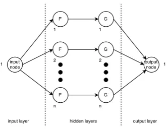
Both hidden layers consists ofnnodes of which each node has only one input. Fed to the nodes of the first hidden layer are N-th order basis functionsFand to the nodes of the second hidden layer a functionG. FunctionGmultiplies the input by a certain weight. The output node gives the resulting sum of all the node outputs of the second layer.
[image:18.595.200.365.171.300.2]To make this more clear, a one-dimensional B-spline network is assumed having a single input. The structure of this network is shown in Figure 2.12.
Figure 2.12:B-spline network structure of 20-sim
For a properly spaced spline domain it is possible to approximate every one dimensional func-tion, see Figure 2.13.
Figure 2.13:Function approximation with B-splines in 20-sim
Training of the network is done by comparing the network output y with the desired output
yd. The observed error between both is used to adapt the weights and the rate at which the
adaptation takes place is defined by the learning rateγ. A quick adaptation can be achieved by using a high learning rate, though for an increased risk of unstable behavior. Forγ=0 the learning is disabled and weight adaptation will not take place.
[image:18.595.198.364.388.475.2]CHAPTER 2. THEORETICAL BACKGROUND 13
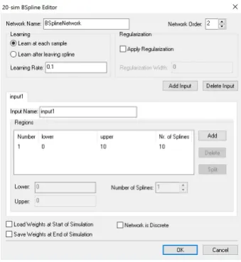
Figure 2.14:The B-spline editor window of 20-sim
The mode "learning at each sample" updates the network weights after each sample (accord-ing to Equation 2.9a). For a certain inputxonly a few splines haveFi(x)6=0, which means
that at each sample only a few weights will be adapted. The mode "learning after leaving a spline" keeps track of inputxand its corresponding non-zero splinesFi(x). Samples of
non-zero splines are stored and only after the input has left the region of a non-non-zero spline its weight will be adapted according to Equation 2.9b.
∆wj=γ·(yd−y)Fj(x) (2.9a)
∆wj=γ·
Pn
i=1 ¡
yd,i−yi¢·Fj(xi)
Pn
i=1Fj(xi)
(2.9b)
In which∆wjrepresents the adaptation of weightwj,γthe learning rate,Fj(x) the basis
func-tion of samplej,xthe input,ydthe desired output andythe network output.
The calculated weights can be saved to file after a simulation experiment has been finished and weights can be loaded from file before the start of a simulation experiment. This makes it possible to use each run different initial data in a multiple run simulation experiment.
2.3.2 B-spline Network with Python Scikit Learn Library
Scikit-learn provides wide functionality and specialized packages for machine learning in Python. The use of those packages makes it possible to analyze data in a simple an efficient way. The packages can be used in various contexts and builds upon NumPy, SciPy and Mat-plotlib, Scikit-learn (2017).
2.3.2.1 SciPy
SciPy is open-source software for science, mathematics and engineering, Scipy Manual (2017). It is a collection of mathematical algorithms and functions that is built on Pythons extension Numpy. One of the sub-packages in NumPy isinterpolatewhich consists of all kinds of in-terpolation functions and methods. From the inin-terpolation package the functionssplrepand
splevare used to implement 1-dimensional B-spline networks and the functionsbisplrep
andbisplevare used for 2-dimensional networks.
curvey=f(x). The function returns the 3-tuple(t,c,k)containing a knotvector, B-spline coefficients and the degree of the spline.
Important to note is that the suppliedxdata must be unique and the array content must con-tain the values in ascending order. Non-unique items should be filtered out before applying data to this function. Furthermore, the knotst must satisfy the Schoenberg-Whitney condi-tions, i.e. there must be a subset of data pointsx[j] such that:
t[j]<x[j]<t[j+k+1] f or j=0, 1, ..,n−k−2 (2.10)
with, t[j] knot at sample j x[j] input at sample j k degree of B-splines
n number of samples
In words, Equation 2.10 tells that in between two consecutive knots of the knotvector a data point must exist.
The function interpolate.splev, Splev (2017) evaluates for some given input x[i] the output value y[i]. In order to evaluate the data the 3-tuple (t,c,k) (the return from
interpolate.splrep()) and the evaluation degree must be supplied. For input values
being outside the defined interval of the knot sequence the returned output will be the extrap-olated value by default, but it is possible to change this to return a 0, to return the boundary value or to raise an error.
The functioninterpolate.bisplrep, Bis (2017b) finds the bivariate B-spline represen-tation of a surface. Data points forx[i],y[i] and z[i] are supplied that describe the surface
z =f(x,y). By supplying the knotvectors t xand t y (optional input) together with a certain B-spline degree the function returns a 5-tuple(tx,ty,c,kx,ky)that contains the knotvec-tors and the degree of thex- andy-dimension and one set of computed coefficientsc. Optional parameters can be set to define the end points of the approximation interval for bothxandy.
The function interpolate.bisplev, Bis (2017a) evaluates a bivariate B-spline (and its derivatives). The only compulsory inputs are the parameters that define the domain over which the spline has to be evaluatedx,yand the 5-tuple(tx,ty,c,kx,ky)(returned from
bisplrep). The return of the function (evaluation) is the cross-product ofxandy. Initially
the evaluation orders ofxandyare set to zero, but those can be changed by definingd x and
d y.
2.4 Illustrative Application: Linear Motor Motion System
The illustrative example used for the thesis is a model of a linear motor motion system. This type of motor is interesting in learning control and is widely used to perform linear motions that require sub-millimeter accuracy (i.e. scanning, laser cutting or pick-and-place tasks), Ot-ten et al. (1997).
2.4.1 Introduction to a Linear Motor
CHAPTER 2. THEORETICAL BACKGROUND 15
Figure 2.15: Working principle of a linear motor. The lines indicate the flux-lines of the permanent
magnets andφa,φbandφcindicate the phases of the 3-phase motor current
The motion is established by applying a three-phase current to three adjoining translator coils. As a result, a series of attraction and rejection forces between the permanent magnets and the coils is generated. The basic behavior of the motor can be seen as the movement of a mass. For the thesis it is assumed that the total mass of the motor including a dummy load defined by
mL=37 [kg].
The translator of the linear motor experiences a force ripple (disturbance) during its operation. The force ripple can be explained by two phenomena that occur:
• Phenomena 1: Cogging force
Between the permanent magnets at the base plate and the translators iron cores a strong magnetic interaction takes place. Disturbance forces that try to align the magnets with the cores into a stable position of the translator cause these interactions. This force is called the cogging force and is independent of the motor current. It depends on the rel-ative position of the translator with the magnets and is even present the moment the motor current is zero. A simplistic model to represent the cogging forceFC[N] is:
FC(x)=10 sin(1.6·10−2x) (2.11)
The equation describes a sinusoidal shaped input disturbance that depends on the mo-tor positionx, has an amplitude of 10 [N] and a pitch of 0.016 [m]. In Figure 2.16 a mea-surement of the cogging of the real motor being modeled is shown.
0 0.1 0.2 0.3 0.4 0.5
Position [m] -15
-10 -5 0 5 10 15
FC
[N]
Cogging
Figure 2.16:Input-output mapping of the position dependent cogging force,FC
• Phenomena 2: Back EMF
Table 2.1:System requirements of the feedback control system (PD controller plus moving mass)
Parameter Value Unit Description
mL 37 kg Total moving mass (linear motor plus dummy load)
¨
xmax 10 m/s2 Maximum acceleration of the mass
emax,t r ack 100 µm Maximum tracking error of the control system
can be generated. Back EMF is generated the moment a coil is moved through a varying electro-magnetic field. If the current supplied to the coils is not proportional to the back EMF, a force ripple will appear.
Using a detailed model of the structure of the motor enables the computation of the back EMF, but in order to do so accurate data about the position and magnetic properties of the permanent magnets is required. In most applications linear motors are used that have large magnetic tolerances (beneficial to reduce the motor costs). For each individual motor the model should be individually adjusted which makes implementing them more difficult. Therefor it is decided to omit the force ripple caused by this fact.
Besides the cogging force, friction and motor inertia are commonly taken into account in modeling a linear motor. An example of a friction force that is encountered is the moment the translator of the motor slides along the guiding rails. The simulations per-formed for this thesis only incorporate the inertia of the mass (together with the cogging force). The friction will be omitted as this force is negligible when compared to the iner-tia.
2.4.2 Design of Linear Motor Model
The model shown in Figure 2.17 is used in simulations to model the linear motor as a plant. It includes the inertia of the mass of the linear motor and the position dependent cogging.
Figure 2.17:Plant model for the non-ideal linear motor in which the inertia of massmLand the cogging are included
2.4.3 Design of Feedback Controller
The feedback controller compensates for random disturbances and generates the learning sig-nal (target) for the LFFC. Tuning a feedback controller is based on certain plant requirements, therefor values are assumed for the maximum allowable tracking erroremax,t r ack, the
maxi-mum possible acceleration ¨xmax of the mass and the total massmL to be displaced, see Table
2.1. An ideal model of a moving mass is assumed for tuning the PD controller.
CHAPTER 2. THEORETICAL BACKGROUND 17
It is chosen to represent the PD controller in serial form as this allows for better tuning in the frequency domain. de Vries (2015) provides the information to design a serial PD controller in transfer function form. The design consists of a combination of the selection of controller gain
KCand a filter formed by specific pole-zero placement ofτz andτp.
CF B=KC· sτz+1
sτp+1
(2.12)
The design starts with defining the cross-over frequency from the maximum acceleration of the mass ¨xmass, the maximum allowable tracking erroremax,t r ackand the tameness factorβ(as a
rule of thumb,β=10):
ωc=
v u u t
¨
xmax·
p
β emax,t r ack
(2.13)
From Equation 2.13 the controller gainKC,τz andτpcan be determined:
KC=
mLω2c
p
β (2.14a)
τz=
q
β· 1
ωc
(2.14b)
τp=
1
p
β·ωc
(2.14c)
The systems cut-off frequency is found to be 562 [rad/s] and the controller transfer function is:
CF B=3.7·106·
5.622·10−3s+1
5.623·10−4s+1 (2.15)
2.4.4 Performance Check on the Feedback System Model
The performance of the designed feedback controller is checked by implementing the feedback controlled system in the simulation software 20-sim. The model is shown in Figure 2.18.
Plant model: ideal linear motor model
y u
uFB
x SP PD
MV s FBcontroller ZOH Hold K 1 mass Reference Sample ∫ v ∫ x
Figure 2.18:20-sim model to check performance of control system
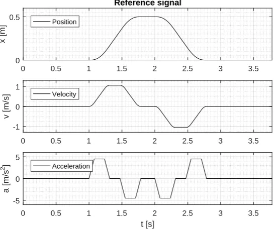
A "MotionProfile" supplies the control system of a partial cubic reference signal having a max-imum acceleration of 10 [m/s2] and a maximum displacement ofxmax=0.5 [m], the complete
Table 2.2:Reference signal parameters for performance check of tuned PD-controller
Parameter Value Unit Description
r i se_t i me 0.527 s Rise time
st ar t_t i me 1.000 s Start time
st op_t i me 1.527 s Stop time
r et ur n_t i me 2.000 s Return time
end_t i me 2.527 s End time
per i od 3.527 s Period of signal
jmax 189.737 m/s3 Maximum jerk
amax 10.000 m/s2 Maximum acceleration vmax 1.581 m/s Maximum velocity
xmax 0.500 m Maximum displacement (= stroke) CV 20 % Percentage Constant Velocity (CV)
C A 20 % Maximum Constant Acceleration (CA)
0 0.5 1 1.5 2 2.5 3 3.5
0 0.5
x [m]
Reference signal
Position
0 0.5 1 1.5 2 2.5 3 3.5
-2 0 2
v [m/s]
Velocity
0 0.5 1 1.5 2 2.5 3 3.5
t [s] -10
0 10
a [m/s
2] Acceleration
Figure 2.19:Reference signal used to check the performance of the tuned PD-controller
The maximum allowable tracking error was defined to be 100 [µm] and from Figure 2.20 it can be observed that this requirement is met.
0 0.5 1 1.5 2 2.5 3 3.5
Time [s]
-1 0 1
Tracking error [m]
#10-4 Tracking error
19
3 Network Communication
3.1 Introduction
A feedback control system can be extended with a feed-forward controller. The most conve-nient way to obtain this is by just implementing both controllers on the same platform, for instance both in the simulation environment of 20-sim. For the thesis the learning controller (feed-forward part) will be implemented in Python. By setting up a network connection be-tween the feed-forward controller in Python and (in this case) the feedback system plus plant in the simulation software 20-sim both can communicate.
The network part is set-up by making use of ZeroMQ, ZeroMQ (2017) and of Protocol Buffer from Google, ProtoBuf (2017). The combination of both enables a well structured data com-munication structure between 20-sim and Python. In this chapter the design of the network layer is presented and its implemented is shown. Two tests are performed to verify if the com-munication works as expected.
3.2 Design of Network Layer
A general feedback control system that is extended with a properly set feed-forward controller shows improved performance. Though it requires both parts to be used on the same comput-ing platform (i.e. Linux, Microsoft Windows or macOS) and all parts needs to be operated in the same operating environment (for instance a simulation environment). To abolish these re-strictions a network layer is added in between the feedback part and the feed-forward part. As a result, both parts can be implemented on different computing platforms. Communication remains possible by setting up a network link. In Figure 3.1 a diagram is shown in which a network layer is included within a learning feed-forward controlled system.
Figure 3.1:Learning feed-forward controlled system that includes a network layer
The feed-forward controller is implemented in Python and contains a function approximator from the Python Scikit learn library. The input-output mapping of the system is adapted during control in order to behave as desired. The feedback part (in this experiment) is implemented in the simulation environment of 20-sim.
The feed-forward controller has to perform three tasks: 1. Collect data
2. Approximate behavior of the inverse plant,P−1(s)
The tasks the feed-forward controller needs to perform do not all require network communi-cation. Only tasks 1 and 3 have to communicate over the network, see Figure 3.2.
Figure 3.2:Tasks of the feed-forward controller, (***) indicates a task requiring network communication
In order to obtain a safe and reliable communication between both sides of the network layer, two protocols are used: ZeroMQ and Protocol Buffer from Google. The latter packs the data into a serialized string such that the data can be sent and received according to one and the same format. The former sends the serialized string over the network. ZeroMQ can be seen as a concurrency framework and is already prepared to carry messages along various trans-port processes (inter-process, in-process, TCP and multicast). The network communication channel is set-up by binding two IP-addresses to each other. At both sides of the network the IP-address of the application containing the feed-forward part must be available.
3.3 Implementation of Network Layer
ZeroMQ, ZeroMQ (2017) and Protocol Buffer, ProtoBuf (2017) from Google are used together to make it possible to transfer data from 20-sim to Python and vice versa. In this section some more information is provided about both protocols.
3.3.1 ZeroMQ
ZeroMQ can be seen as a concurrency framework that provides sockets to carry messages across various transports, i.e. inter-process, in-process, TCP and multi-casts. It can connect N-to-N sockets according to several patterns such as fan-out, pub-sub and request-reply. The latter is used to bind both applications together and a connection between client (20-sim) and server (Python) needs to be set-up manually. This is done by providing the IP-address of the server to the client application, which must be contained in the config file (.cfg) that will be automatically read as soon a simulation is started.
CHAPTER 3. NETWORK COMMUNICATION 21
Figure 3.3:ZeroMQ communication diagram between client and server. Three network communication actions in the order 1) connect, 2) client request (REQ) and 3) server reply (REP)
3.3.2 Protocol Buffer from Google
Protocol Buffer from Google is used to serialize data in a structured way (creating a message) with its property of being language and platform neutral. The structure of the data only has to be defined once and after that the special generated source code can be used to write and read data from the structure using variety of languages and from variety of data streams.
The data structure of the message is specified by defining a protocol buffer message of the type
.proto. The message is small and forms a logical record of information contained in a series
of name-value pairs. Each message type has one (or more) uniquely numbered fields defined by a name and a value type. Possible value types are for instance booleans, numbers, raw bytes and strings. The fields can be specified as optional, required and repeated fields as well.
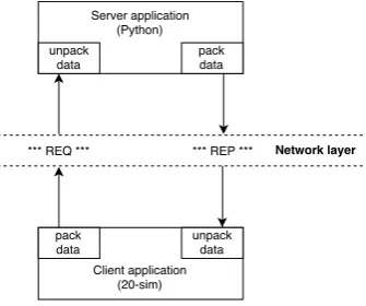
In the control systems client-server setting, before the client actually sends out its request (REQ) the data is packed into a message (containing a serialized string) by Protocol Buffer. The server receives the request and unpacks the message using Protocol Buffer such that actions can be performed on the data. The new data is packed by Protocol Buffer into a message which is send as a reply (REP) back to the client. The client receives the reply, unpacks the data again with Protocol Buffer. The data is ready to be used by 20-sim. The packaging structure is illus-trated in Figure 3.4.
[image:27.595.218.386.524.664.2]3.3.3 Network Communication with 20-sim
The feedback control system is implemented in the simulation environment of 20-sim. Since it is not possible to directly communicate with 20-sim from an external application a DLL is used to make this possible. A DLL is a Dynamic Link Library and is a file that contains instructions that can be called by another program to perform a certain task (for instance tasks requested by 20-sim). It is not possible to run a DLL file directly (like an executable file,.exe) but it must be called by some other running code. The term ’dynamic’ refers to the fact that the data within the file is only used the moment a program actively calls the data. As a result, the data is not always available in memory. In order to run simulations in 20-sim that include network communication, the program is required to perform a DLL call to a.dll(created by a build of code written in C++) such that via that file a temporarily communication link is opened to the Python server, and vice versa. A DLL call in 20-sim can be done as follows:
output=dll(dll_name,function_name,input) (3.1)
with, dll_name: the name of the DLL file with extension.dll
function_name: the name of the function containing the action to be performed
input: input data to be passed on the function that is called
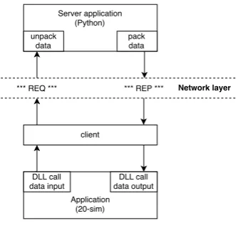
[image:28.595.202.368.383.543.2]This function returns data that is configured asoutput. It is possible to perform calls that pass on single or multiple inputs and/or that receive single or multiple outputs. The diagram in Figure 3.5 visualizes a DLL call between the 20-sim client and the Python server.
Figure 3.5:Diagram of DLL call from 20-sim to Python server
The 20-sim simulation software supplies the user with a standard structure for making a DLL call. A Visual C++ code example is provided 20simDynamicDLL (2017) which can be used and modified to achieve specific functionality. In considering a multiple run simulation experiment the actions that are consecutively performed by the simulation are:
1. Initialize()
Function called by 20-sim before the simulation experiment is started, and only once in a multiple run experiment. Initializations of data structures can be placed within this function.
2. InitializeRun()
CHAPTER 3. NETWORK COMMUNICATION 23
3. dllFunction()
Function called during a simulation experiment in which for instance data can be cap-tured and modified.
4. TerminateRun()
Function called by 20-sim after each finished run. For instance, clean-up of data can be done within this function.
5. Terminate()
Function called by 20-sim after a finished (multiple run) simulation experiment.
The above structure will be used to create an efficient communication between the 20-sim client (making a DLL call) and the Python server. This structure will ensure that actions only take place the moment they need to.
3.4 Validation of Network Layer
The proposed network communication set-up is evaluated by performing two tests. One to see if a server (in Python) and a client (in C++) can communicate with each other by sending each other a string. The second test will verify if 20-sim can make a DLL call to a.dll-file that was created by building a program written in C++. For this test a simulation in 20-sim is started and data is send to the Python server. The server manipulates the received data and send it back to the client.
For both tests two devices (laptops) are connected to the same network and both IP-addresses are within the same subnet. This way it is enabled that both devices are allowed "to see" each other and the possibility arises to set-up a connection between them. The IP-addresses of the client and server areIPv4:192.168.0199andIPv4:192.168.0.200. At both applica-tions the IP-address of the server needs to be known. At the server side, the IP-address used is referred to by using local host and at the client side a.cnf(config) file is read out in which the IP-address of the server needs to be inserted manually.
3.4.1 ZeroMQ Test
The "ZeroMQ test" is a test to validate if it is indeed possible to let a client implemented in C++ communicate over the network to a server implemented in Python. The client will send the string "Hello" and it is intended to receive the string "World" back from the server. The ZeroMQ connection is based on the Request-Reply (REQ-REP) mode. To validate if it works, the server in PythonZeroMQ_server.pyis started followed by executing the clienttestZeroMQ.exe. The output of the server is shown in the "IPython console" and the output of the client appears in the command prompt window, see Table 3.1.
Table 3.1:Ipython console output and command prompt window output, after completed communica-tion between client and server
testZeroMQ_server.py testZeroMQ.exe
Received request: b’Hello’ Reading IPaddress from file...
Connecting to hello world server ... Sending Hello
Received World
Figure 3.6:Wiresharkpackage flow for communication between client and server
Table 3.2:Part of the package content containing "Hello" and "World", data extracted usingWireshark
Source IP Destination IP Information
192.168.0.199 192.168.0.200 [PSH, ACK] Seq=65 Ack=92 Win=65536 Len=49
[TCP segment of reassembled PDU]
TCP payload (49 bytes): containing Hello
192.168.0.200 192.168.0.199 [PSH, ACK] Seq=114 Ack=144 Win=65536 Len=9
[TCP segment of reassembled PDU]
TCP payload (9 bytes): containing World
3.4.2 Data Transfer Test
The "data transfer" test is performed to see if the simulation software (20-sim) can commu-nicate with a server in Python, by performing a DLL call. 20-sim makes a call to the function
dataTransfer, a request (from the client) is send to the server and a reply is received back
from the server.
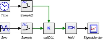
A 20-sim simulation is started in which a reference input signal 2 sin(t) is used,t∈[0, 2π]. The block "DLLcall" contains the function to make a DLL call (using 3.1) such that a communication link between the Python server and the client is established. Input for the function are samples of the reference input and the time obtained by using a sample time of 0.01 [s]. The purpose of the experiment is that Python receives the sampled data, multiplies the references signal by two and sends back the result to 20-sim. The simulation model used is shown in Figure 3.7.
K
callDLL
ZOH
Hold Sample
Sample2
SignalMonitor Sine
Time
Figure 3.7:20-sim model used to perform the data transfer test for communication between 20-sim and Python
CHAPTER 3. NETWORK COMMUNICATION 25
0 2 4 6
Time [s] -4
-3 -2 -1 0 1 2 3 4
Value []
Client
output input
0 2 4 6
Time [s] -4
-3 -2 -1 0 1 2 3 4
Value []
Server
input output
Figure 3.8:In- and output data plotted at a) client side (20-sim) and b) server side (Python)
3.5 Conclusion
The client (C++) and server (Python) in the "ZeroMQ test" correctly communicate, the client sends the string "Hello" to the server, the server receives it and sends "World" back to the client (and receives it).
The "data transfer" test showed that 20-sim was able to correctly communicate to the server by a DLL-call . To do so, a simulation was started in which an input signal (2 sin(t)) was generated, sampled and send to the server.
It can be concluded that the combination of ZeroMQ and Protocol Buffer from Google can be used to set-up a network communication link between 20-sim and Python.
4 One Dimensional LFFC
A feedback control system that is extended with a properly set 1-dimensional (1D) learning feed-forward controller shows improved system performance. Depending on the input signal supplied to the learning controller it is suited for repetitive motions or non-repetitive motions. A time-indexed LFFC (input is a function of the periodic motion time) is used for repetitive motions and a state-indexed LFFC (input is the reference position, velocity or acceleration) is used for non-repetitive motions.
This chapter starts with the design of two 1-dimensional time-indexed learning feed-forward controllers for which the environment in which they are implemented differ. For both imple-mentations the reference signal is produced by the built-in "waveform generator" of 20-sim and the signals shape it produces is referred to as a partial cubic motion. A general feedback system is used in which a tuned PD-controller controls the ideal plant model representing a moving mass.
The feed-forward part contains a learning controller that will approximate the mass of the plant by using a B-spline Network. The difference between both time-indexed LFFCs is found within this part. One implementation uses the built-in B-spline Network editor of 20-sim and the other uses the Scikit-learn library from Python. The latter implementation requires the set-up of a network connection between 20-sim and Python, for more details see Chapter 3.
Both implementations are compared by evaluating the simulation results obtained by 20-sim, but also the user friendliness and the design freedom during those simulations is taken into account. A time-indexed LFFC is implemented using Python only and the task of the learning controller is to learn the inverse behaviour of the plant, i.e. its mass.
The designed time- and state-indexed LFFCs have the B-spline networks designed using pa-rameters which seem to cause no instable behavior. Though, it might be possible that for in-stance by extending the simulation periods and/or the number of runs (within a multiple run session) unstable behavior will occur. Designing a perfect LFFC is beyond the scope of this thesis.
4.1 Time-Indexed LFFC
Time-indexed learning feed-forward controllers are beneficial for linear motor motion systems that has to perform repetitive motions. This type of motions will observe at each time instance the same plant influences and other disturbances each time the motion repeats. Therefor, the input supplied to the learning controller can be chosen to be a function of the periodic motion time,Tp for which the motion is defined on the input domaint∈[0,Tp]. The structure of a
time-indexed LFFC is shown in Figure 4.1.
Figure 4.1:Time-indexed LFFC structure (1-dimensional)
4.1.1 Design
CHAPTER 4. ONE DIMENSIONAL LFFC 27
Table 4.1:Trainings signal parameters time-indexed LFFC
Parameter Value Unit Description
Tr i se 0.786 s Rise time
Tst ar t 1.000 s Start time
Tst op 1.786 s Stop time
Tr et ur n 2.000 s Return time
Tend 2.786 s End time Tp 3.786 s Period of signal
jmax 57.276 m/s3 Maximum jerk
amax 4.500 m/s2 Maximum acceleration vmax 1.061 m/s Maximum velocity
xmax 0.500 m Maximum displacement (= stroke) CV 20 % Percentage Constant Velocity (CV)
C A 20 % Percentage Constant Acceleration (CA)
has to learn the inverse behavior of the ideal plant for which a model is used that incorporates the inertia of the massmL only. A more detailed description of the plant model is given in
Section 2.4 and the model itself is shown in Figure 4.2.
Figure 4.2:Ideal plant model of linear motor
The parameters to be selected are the upper and lower input values, the learning rate, the num-ber of B-splines, the distribution of the B-splines and the degree of the B-splines. Especially the number of B-splines and the learning rate are important to select properly, because those pa-rameters influence the stability of the learning controller. The B-spline network setting are determined according to the following step-by-step plan:
Step 1: Input selection of the BSN
The input selection for the BSN is based on the motions to be performed by the linear mo-tor. Since a time-indexed LFFC shows only good performance for repetitive motions inputtis selected for the learning controller, which is a function of the periodic motion timeTP.
Step 2: Selection of the B-spline order
Along with the degree of the B-splines the smoothness and accuracy of the function approxi-mation is set. The higher the degree the more complex the computation of the B-splines and therewith the longer the process time will be. First degree (or second order) B-splines will be used.
In using this type of basis functions a smooth enough approximation can be achieved while limiting the computational complexity, as suggested in Velthuis (2000). First degree B-splines are described by two linear line segments forming a triangular shape, see Section 2.2.1.
Step 3: Selection of the trainings motion
0 0.5 1 1.5 2 2.5 3 3.5 0 0.5 x [m] Reference signal Position
0 0.5 1 1.5 2 2.5 3 3.5
-1 0 1
v [m/s]
Velocity
0 0.5 1 1.5 2 2.5 3 3.5
t [s]
-5 0 5
a [m/s
[image:34.595.146.420.83.313.2]2 ] Acceleration
Figure 4.3:Trainings motion for the time-indexed LFFC (acceleration) and derivatives thereof
Step 4: Selection of the B-spline distribution and the number of splines
The distribution of the B-splines will be uniformly, which means that each B-spline is equally spaced over the input domain from [0,TP]. Reason for this is that it is more easily to implement
while still sufficient simulation results can be obtained. Besides that, in 20-sim it is not possible to define a non-uniform B-spline distribution.
In most situations an exact model of the plant is not available. In order to be able to still de-termine the minimum B-spline width of the network the step-by-step plan given in "Algorithm 2.3", Velthuis (2000) can be used:
4.1: Find infinity norm of the inverse complementary sensitivity function The infinity norm is defined as¯¯−T(jω)
¯ ¯
∞. The inverse complementary sensitivity
func-tion−T(jω) (closed system) is used to determine this norm. In Figure the diagram is shown from which is found that:
¯
¯−T(jω) ¯ ¯
∞=1.275[d B] (4.1)
4.2/4.3: Find the minimum frequency for which the cosine of the Phase (Step 4.1) is smaller or equal than zero
In Figure 4.5 cos(φ) is shown in whichφrepresents the phase obtained from¯
¯−T(jω) ¯ ¯
∞
(shown in Figure 4.4). The minimum frequency for which cos(φ)≤0 is:
min
ω∈R|cos(φ≤0) ¯
¯−T(jω) ¯
¯→ω=852.699[r ad/s] (4.2)
The smallestω1at whichφ1=arg(−T(jω1)) satisfiesφ1=arccos ³
−0.0147 |−T(jω)|∞
minω∈R|cos (φ≤0)|−T(jω)|
´
is found using Step 4.1 and Step 4.2:
φ1=arccos Ã
−0.0147
¯
¯−T(jω) ¯ ¯
∞
minω∈R|cos (φ≤0) ¯
¯−T(jω) ¯ ¯ !
=
µ
−0.0147·1.275 [dB]
1.122 [dB]
=91.074 [deg]
CHAPTER 4. ONE DIMENSIONAL LFFC 29
100 101 102 103 104
frequency [rad/s] -60
-40 -20 0 20
magnitude [dB]
Magnitude
100 101 102 103 104
frequency [rad/s] 0
50 100 150 200
phase [degree]
Phase
Figure 4.4:Bode diagram of the inverse complementary sensitivity function, i,e.¯
¯−T(jω)
¯ ¯
∞(from the
closed loop system)
100 101 102 103 104
frequency [rad/s] -1
-0.8 -0.6 -0.4 -0.2 0 0.2 0.4 0.6 0.8 1
cos(
?
)
cos(?)
4.4: Find the minimum B-spline widthdmi n
Using the obtainedω1(from Step 4.2/4.3) the minimum widthdmi nof the B-splines is
determined according to:
dmi n=
2π
ω1 →
dmi n=
2π
852.699=7.369·10
−03 (4.4)
By dividing the motion periodTp=3.78 [s] bydmi nthe maximum number of B-splines
is obtained:
Nmax=
Tp
dmi n →
Nmax=
3.78
7.369·10−03 =512 (4.5)
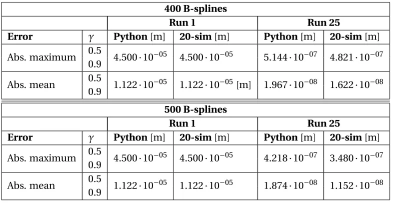
The number of splines must be lower than 512. In order to compare the BSN implemen-tations of 20-sim and python two values are chosen, i.e. 400 splines and 500 splines.
In Figure 4.6 the uniform distribution ofN B-splines of second order (degree zero) is shown. The basis functions are sequentially labeled byi∈1...N. The distribution shows that the first (1) and last (N) basis function have half the width of the basis functions at the center part. This type of learning controller is used for performed motions that are completely independent. This means that before a new motion is started, the system is brought back to its initial states. A typical application in which this type of "reset" is used is a pick-and-place machine.
Figure 4.6:A B-spline distribution of time-indexed LFFC
Step 5: Selection of the learning rate
The learning rate of the feed-forward controller is wished to be as large as possible such that convergence is reached fast. Though, too high rates may result instable behavior. In Velthuis (2000) an equation is proposed in order to determine the maximum possible learning rate:
γ≤¯ 2
¯−T(jω) ¯ ¯
∞
→γ≤0.948 (4.6)
For the simulations the learning rates are set toγ=0.5 andγ=0.9, both lower than the maxi-mum allowable value found from Equation 4.6 to avoid unstable behavior.
4.1.2 Implementation
CHAPTER 4. ONE DIMENSIONAL LFFC 31
4.1.2.1 B-spline Network with 20-sim B-spline Editor
In this section the built-in B-spline network editor (from the software 20-sim) is used to im-plement the B-spline network in the feed-forward part of the control system. In Figure 4.7 the 20-sim model used for this is shown. The plant model only includes the influence of the inertia of the massmL=37 [kg].
Bspline network
uFF
y uFB
ideal part Plant model: linear motor
u a y v x a v t uFF uFB K dataCollection PD SP MV s FBcontroller ZOH Hold K 1 mass MotionProfile Sample1 Sample2 Sample3 Time ∫ v ∫ x
Figure 4.7:20-sim model for time-indexed LFFC using 20-sim implementation with ideal plant
The built-in waveform generator of 20-sim is used to supply inputx to the model, see Fig-ure 4.3. The input for the B-spline network ist sampled each millisecond. Furthermore, the network is supplied with the so called target signal. This signal is the output of the feedback controller multiplied with the learning rate (γ) plus the feed-forward signaluF F pr evi ous of the
previous run (at a specific sample instance). The moment no previous data is available signal
uF F pr evi ous=0.
Depending on the observed tracking error (difference between the system output y and the desired outputyd) and the learning rate the B-spline network will adapt its network weights.
The output of the B-spline network is the feed-forward control signal,uF F, that is fed into the
control system just before the input of the plant.
The function approximation is performed by the BSN in 20-sim and therefor the "dataCollec-tion" block is used only to send the collected data over the network to the Python server. The server saves the data to file in (.txt) format. The collected data is the timet [s], reference inputs (x[m], ˙x=v[m/s], ¨x=a[m/s2]), feedback outputuF B[N], feed-forward outputuF F[N]
and the system outputy[m].
4.1.2.2 B-spline Network with Python Scikit-Learn
The model used to implement the Python B-spline network is shown in Figure 4.8. The plant model includes the inertia of the mass only.
ideal part Plant model: linear motor
u x uFB uFF y x t y v a v a uFB uFF PD SP MV s FBcontroller K FFcontroller ZOH Hold K 1 mass MotionProfile Sample1 Sample2 Sample3 Time ∫ v ∫ x
Figure 4.8:20-sim model for time-indexed LFFC implemented with a Python B-spline network