2D Quench propagation modelling in COMSOL

1

2D Quench propagation modelling in

COMSOL

Nils Jansen van Rosendaal (SET) s1122908

University of Twente, TNW, EMS UT supervisor: Marc Dhallé

CERN, ATLAS magnet group Geneva, Switzerland 14 April - 14 October 2016

2

Abstract

A 2D quench propagation model in COMSOL, based on earlier work by Volpini [1], was developed and results were compared to literature. The model was used to calculate the quench propagation velocity and minimum quench energy for aluminum stabilized NbTi superconducting cables for different current levels and RRR values for the stabilizer. Both single cable and coil simulations were performed to simulate the ECT and BT conductors used in the ATLAS B00 test coil. Quench

3

Table of Contents

Abstract ... 2

Introduction ... 4

Simulation of B00 test coil ... 5

Cable geometry ... 7

Single cable simulations ... 8

Full sub-coil simulations ... 10

Material properties ... 10

Mesh ... 14

Results ... 15

Discussion... 22

Conclusion ... 22

References ... 23

Nomenclature ... 25

4

Introduction

In particle physics experiments, large detector magnets are used to provide the magnetic field required to identify charged particles formed during collisions and to determine their momentum. At CERN, plans are being developed for the FCC (Future Circular Collider), of which the collision energy will be 7 times higher than that of the currently operating LHC (Large Hadron Collider). For this purpose, designs for suitable detector magnets are required [2]. Important design aspects of a detector magnet are the stability and quench behavior. Above a critical temperature, depending on the magnetic field, the current and the conductor used, a superconductor transitions to the normal state so that any current flowing through the conductor results in ohmic dissipation. A normal zone can be caused by a local temperature increase exceeding the current sharing temperature. If the normal zone is large enough (exceeding the so-called minimum propagation zone), it will continue to heat up and expand, which may cause permanent damage to the coil. This process is called a

quench. To reduce the chance of a quench occurring and to subsequently reduce the amount of local heating in case of a quench, stabilizer materials, highly conductive metals surrounding the

superconductor, are used. The stability of a superconducting cable or coil can be described with the minimum quench energy (MQE), the amount of heat it can absorb before it quenches.

Throughout the years, detector magnets have developed and were improved in several ways to form a mature technology. The driving force behind the development is the requirement for larger and more powerful magnets, to be able to detect particles of higher energies while maintaining a high reliability. One common feature of modern detector magnets is the usage of superconducting Rutherford cables made of strands comprising niobium-titanium in a copper matrix, stabilized with aluminum [3]. In the CMS detector magnet and the ATLAS central solenoid at CERN, the aluminum was reinforced to become part of the structural design so that only a fraction of the hoop stresses are transferred to the support cylinders [4] [5]. For CMS, pure aluminum with a high RRR was used as a stabilizer and high strength, low RRR aluminum was used to reinforce the conductor. For the ATLAS central solenoid, nickel was added to high purity aluminum to yield a material with both high yield strength and high RRR. It is possible to combine these two methods [6] [7], which is of practical interest for future ultra-thin detector magnets.

5

Simulation of B00 test coil

To verify the validity of the model, the conductors in the ATLAS B00 test coil are simulated and the results are compared to measured values of the MQE and QPV. The B00 test coil was originally created to test the End-Cap Toroid (ECT), Barrel Toroid (BT) and Central Solenoid (CS) conductors to be used in the ATLAS experiment at CERN. Measurements on MQE and QPV were conducted on the ECT and BT cables, which can be seen in Figure 1. A schematic representation of a single aluminum-stabilized NbTi superconductor can be seen in Figure 4 (left). The cable comprises the NbTi/Cu Rutherford cable and the highly conductive aluminum stabilizer surrounding it. The dimensions for the BT and ECT conductor are shown in Table 1.

Figure 1 Schematic cross-section view of the B00 test coil [10]

Based on the model by Volpini, an improved 2D quench propagation model has been made. The key improvements are the incorporation of the NbTi and copper into the model, as well as insulation and the use of multiple layers of conductors, which is believed to be more physically correct. The main equation of the model, equation (3), is still the same as in the original model and is shown below.

𝜌_𝑚𝐶_𝑝𝜕𝑇

𝜕𝑡+ ∇ ∙ (−𝑘∇𝑇) = 𝜌 𝐼2

𝐴2 (1)

𝐽⃑ = 1

𝜇₀∇ × 𝐵⃑⃑ (2)

𝜌_𝑚𝐶_𝑝𝜕𝑇

𝜕𝑡 + ∇ ∙ (−𝑘∇𝑇) = 𝜌 ( 1

𝜇0∇ × 𝐵⃑⃑) 2

(3) The equation is composed of equation (1), which contains a heat accumulation and a diffusion term on the left and an ohmic dissipation term on the right, and of equation (2), which replaces the dissipation term with a function of magnetic field instead of current. In this way, the electromagnetic diffusion of the current from the superconductor into the stabilizer, which cannot be assumed to be infinitely fast, is taken into account. Because of the relatively slow current diffusion, mainly limited by inductive effects, it takes time before the current is spread out evenly through the aluminum stabilizer during a quench. This results in a temporary greater concentration of current in the aluminum directly around the core, generating extra heat. This effect influences the quench propagation velocity and minimum quench energy, as argued by Volpini [1].

6

To illustrate this, 1D approximations of the QPV for the B00 BT and ECT conductor were calculated assuming infinitely fast current diffusion through the conductor cross-section during a quench. For this approximation equation (4) was used, which is an adiabatic solution to equation (1), as shown in [1] and [11]. Equation (4) is normally used for simulating adiabatic superconducting strands of a small diameter, where the assumption of infinitely fast current diffusion is more valid because the short diffusion path.

𝑄𝑃𝑉 = 𝐽𝑜𝑝 𝜌_𝑚𝐶_𝑝√

𝜌 𝑘

𝑇_𝑡− 𝑇_𝑜𝑝 (4)

In the equation 𝑇𝑡= (𝑇𝑐𝑠+ 𝑇𝑐)/2. The results for the 1D approximations at different current levels,

along with measurement results from [12], are shown in Figure 2 and Figure 3. It can be seen that the 1D approximation yields too low QPV values, as is to be expected because current diffusion is not taken into account. The use of a 2D model that takes the current diffusion into account is therefore appropriate in this case.

Figure 2 1D quench propagation velocity approximation versus measurement data for the B00 BT conductor using RRR = 3000 for the aluminum stabilizer [12]

Figure 3 1D quench propagation velocity approximation versus measurement data for the B00 ECT conductor using RRR = 3000 for the aluminum stabilizer [12]

0 5 10 15 20 25

0 5 10 15 20 25 30

QPV

(m

/s

)

Current (kA)

B00 BT quench propagation velocity, RRR = 3000

Measurements 1D approximation

0 5 10 15 20 25

0 5 10 15 20 25 30

QPV

(m

/s

)

Current (kA)

B00 ECT quench propagation velocity, RRR = 3000

7 Cable geometry

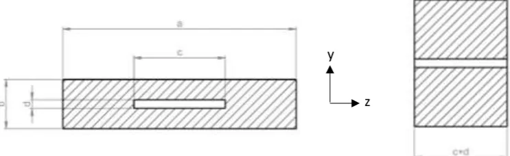
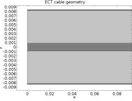
Figure 5 shows the lay-out of the 2D single cable model. Part of a single ECT cable with insulation can be seen. The center part of the image represents the superconducting core, it is surrounded by aluminum stabilizer and around that a thin layer of insulation can be seen. Because a 2D model is used to approximate the 3D geometry of the cable, the thicknesses of the core and aluminum stabilizer were adapted as shown in Figure 4. This was done to assure that the heat capacity of the core and stabilizer has the correct ratio and the current diffusion length is close to that of the real cable. For the model, ‘average’ thicknesses for the conductor and its core were used. The thickness of the Cu/NbTi core in the simulation was calculated by dividing its area (c x d in Figure 4) by half its circumference (c + d). The thickness of the aluminum was calculated by dividing its area (a x b – c x

d) by half the circumference of the core as well. These dimensions were chosen so that the contact

area between the core and the stabilizer in the model matches that of the real cable. In this way the current density during a quench has the most realistic value. Note that in the model the width of the cable in the z-direction is infinite, the width c + d is only used to adjust the thickness in the

y-direction.

Figure 4 Schematic cross section of a superconducting cable with aluminum stabilizer (shaded) and NbTi/Cu core (white) (left) and the corresponding ‘cross section’ used in the 2D model (right). Note that the actual width of the cable in the

z-direction in the model is infinite.

The thickness of the insulation was not changed and is therefore 0.25 mm (so 0.5 mm between two adjacent conductors). The material properties for the insulation were altered to correct for heat capacity and thermal conductivity, as will be discussed under ‘Material properties’ . The used length for the single conductor simulations is 8 m, except at low currents where it is 16 m. This is to allow for the normal zone propagation to reach a steady state, which requires more cable length because the MPZ is larger at low currents.

8

Table 1 Dimensions of the B00 ECT and BT conductor [8] [10] [12]

B00 ECT B00 BT

Dimensions (a x b) 41 x 12 mm 57 x 12 mm

Number of strands 40 32

Core dimensions (c x d) 27.88 x 2.3 mm 22.3 x 2.3 mm

Figure 5 (Part of) lay-out of COMSOL model of a single ECT cable with aluminum stabilizer in light grey and core and insulation in dark gray

Single cable simulations

For a single cable without insulation, the boundary conditions are shown in Table 2. Because in the 2D model the cable is infinitely wide in the z-direction, only the Bz component of the magnetic field

has to be taken into account. This simplifies the model and its boundary conditions. Similar to Volpini [1], equation (2)can be rewritten as:

𝐽_𝑥 = 1 𝜇0(

𝜕𝐵_𝑧 𝜕𝑦 −

𝜕𝐵_𝑦 𝜕𝑧) =

1 𝜇0

𝜕𝐵_𝑧 𝜕𝑦 𝐽_𝑦= 1

𝜇₀( 𝜕𝐵_𝑥

𝜕𝑧 − 𝜕𝐵_𝑧

𝜕𝑥) = − 1 𝜇₀

𝜕𝐵_𝑧 𝜕𝑥

𝐽_𝑧= 1 𝜇₀(

𝜕𝐵𝑦

𝜕𝑥 − 𝜕𝐵_𝑥

𝜕𝑦) = 0

(5)

Because Jy = 0 at y = ±thcable/2 and t = 0, Jx from equation (5) can be rewritten and integrated to yield:

𝐵_𝑧 = 𝜇₀∫ 𝐽_𝑥𝑑𝑦 = 𝜇₀𝐽_𝑥𝑦 (6)

The boundary conditions for Bz as shown in Table 2 can be easily derived from this expression, the

equations at t = 0 describe the current density inside the core in terms of a changing magnetic field and the field remains constant outside the core as there is no current there. These constant values remain constant at all times at y = ±thcable/2 because the amount of current running through the

9

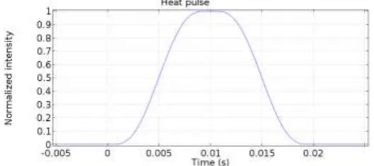
The temperature at t = 0 is equal to the operating temperature of the magnet, which is 4.8 K [12]. A heat pulse is released to trigger the quench in the model. This is represented as the function f(t) in the boundary conditions, with P the power of the pulse and 0.1 Ccore the contact area of the heater

on the conductor. The heat pulse is modelled after the quench heater used in the B00

measurements. It is located at the first 10cm of the conductor and the pulse duration is less than 20 ms, which is less than the normal zone formation time so that pulse duration does not affect the MQE [12]. The pulse is a rectangular function of time with smoothened edges and can be seen in Figure 6. The duration of the pulse in the model is longer than the pulse used in the measurements (4.5 ms) and the pulse is smoothened to prevent large temperature gradients from occurring in the model. This is because larger gradients require more elements to be able to correctly solve the model.

Figure 6 Normalized heat pulse as a function of time

The rest of the thermal boundary conditions make the simulation adiabatic. The boundary condition in T at x = 0 is a symmetry condition, as a normal zone propagates in two directions in a symmetric fashion. The condition at x = L is put in place to make sure the model can be solved, but is not realistic for the single cable simulations, because the heat capacity beyond it is not taken into account. It is therefore important to only use simulation results at a time smaller than the time it takes for any heat to travel to this point, so T(x = L, t)

≯

y-direction around y = 0 for a single cable, only half of each single cable has to be simulated, with

Bz = 0 at y = 0. Computation time is saved by doing so, because less elements are used in the

simulation.

Table 2 Boundary conditions for a single cable without insulation

𝑡 = 0 (𝑦 < 0) 𝐵𝑧 = −𝜇0𝐽𝑜𝑝min (abs(y), 𝑡ℎ_{𝑐𝑜𝑟𝑒}

2 )

(𝑦 > 0) 𝐵_𝑧 = 𝜇₀𝐽_𝑜𝑝min (y,𝑡ℎ𝑐𝑜𝑟𝑒 2 )

𝑇 = 𝑇_𝑜𝑝

𝑦 = −1

2𝑡ℎ𝑐𝑎𝑏𝑙𝑒 𝐵𝑧 = −

𝜇0𝐽𝑜𝑝𝑡ℎ𝑐𝑜𝑟𝑒

2 (𝑥 < 0.1)

𝑑𝑇 𝑑𝑦= 𝑃

𝑓(𝑡) 0.1𝐶_{𝑐𝑜𝑟𝑒}

𝑦 =1

2𝑡ℎ𝑐𝑎𝑏𝑙𝑒 𝐵𝑧 =

𝜇₀𝐽_𝑜𝑝𝑡ℎ_{𝑐𝑜𝑟𝑒} 2

𝑑𝑇 𝑑𝑦= 0

𝑥 = 0 𝑑𝐵𝑧

𝑑𝑥 = 0

𝑑𝑇 𝑑𝑥 = 0

𝑥 = 𝐿 𝑑𝐵𝑧

𝑑𝑥 = 0

10

Full sub-coil simulations

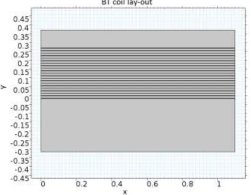
The 2D full coil model shown in Figure 7 is a stack of 10 single BT cables with insulation, consistent with the number of turns used in the B00 coil for both the ECT and BT sub-coils. Note that only one of the two pancakes of the original sub-coil is simulated, due to symmetry. The bottom layer represents the most inner turn, where the heat pulse is released in the first 10cm on the left, as in the single cable simulations. Ground insulation is added at the top and bottom layer and large surfaces representing the aluminum case of the coil are present. The thickness of the ground insulation in the B00 coil is unknown and was put to 2mm for both the ECT and for the BT

simulation. The used length of each layer is 1.1 m, which is the length of the most inner turn of both the ECT and the BT sub-coils. Periodic conditions have been added, ensuring the temperature profile at the end of each layer (right side) equals that at the start (left side) of the next one above it. The other boundary conditions of each layer are equal to that of the single cable boundary conditions described above.

Figure 7 Lay-out of full BT sub-coil model with casing

In the insulation region of the model, equation (3)has been adapted in recognition of the absence of current flow in that region. The right-hand term has been removed from the equation inside the insulation so that ohmic dissipation cannot occur. The resulting equation, equation (7), is shown below.

𝜌𝑚𝐶𝑝

𝜕𝑇

𝜕𝑡+ ∇ ∙ (−𝑘∇𝑇) = 0 (7)

Material properties

11

Table 3 B00 properties

Strand diameter 1.3 mm [10] Cu : NbTi ratio 1.3 : 1 [13]

RRR Aluminum at 0T 3000 RRR Copper at 0T 80 [8]

Operating temp. 4.8 K [12]

The aluminum stabilizer absorbs and conducts heat and current during a quench. It is favorable for the aluminum to have a high RRR, so that heating is limited and thermal diffusion more pronounced. Very high purity aluminum was used for both the ECT and the BT cable in the B00. The RRR of the used aluminum is estimated at 3000. Simulations at RRR = 1100 were also performed to gain insight in the effect of RRR on stability and quench propagation velocity. The density of the material is fixed at a constant value of 2698kg/m3 _{and the temperature-dependent heat capacity is considered. The} electrical resistivity and thermal conductivity are both temperature and magnetic field dependent and are shown in Figure 8 for different fields. It is clear that the relation between these properties and the magnetic field is nonlinear.

Figure 8 Electrical resistivity (left) and thermal conductivity (right) of aluminum for different magnetic field strengths

To verify the accuracy of these values obtained in Cryocomp, a comparison with literature was made. Extensive literature on the temperature dependence of the resistivity and thermal

conductivity of aluminum and the relation between them is available [14] [15] [16]. Literature on magnetoresistivity of aluminum is also available [17] [18] [19]. However, only limited confirmation of the used material properties was found, because the required combination of temperature range, magnetic field and RRR is only partially covered by the literature found. For the resistivity and thermal conductivity at 0T the literature values were found to be consistent with the Cryocomp data. For the magnetoresistivity two articles matched the Cryocomp data [17] [18]. The third article was off by a factor two and also in disagreement with the other literature [19]. The overall

conclusion is that the Cryocomp data is in general agreement with literature.

12

The core in the model consists of three materials: the NbTi superconductor, the copper matrix and a small fraction of aluminum stabilizer, for all of which the material properties are taken from

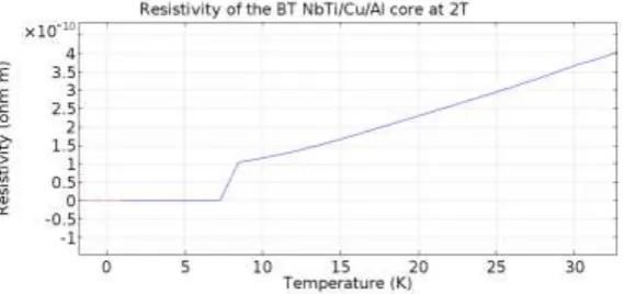
Cryocomp. Comparison with literature [11] [16] [20] of the material properties of copper obtained through Cryocomp showed good agreement for all properties. For NbTi the Cryocomp data and literature [11] also agreed well. The temperature and magnetic field dependence of the resistivity and thermal conductivity of copper, for RRR at zero magnetic field equal to 80, are shown in Figure 9. The ratio of the copper and NbTi is 1.3 : 1 and the aluminum takes the space in the c x d rectangle described in Figure 1 that is not occupied by the NbTi/copper strands. This results in a NbTi : Cu : Al ratio of 0.360 : 0.468 : 0.172 in the core. Average values according to this ratio are used for the density, heat capacity and thermal conductivity. For the electrical resistivity the parallel value of the three materials is used, above the critical temperature. Between the current sharing temperature and the critical temperature an extra term to take into account the current sharing behavior is added. Below the current sharing temperature the resistivity is put to a negligible value of 10-30 _Ω∙m to represent the superconducting state. This results in the expressions below in equation (8) of which the result for the BT cable at 2T is shown in Figure 10.

(𝑇 < 𝑇𝑐𝑠) 𝜌(𝑇) = 10−30

(𝑇_𝑐𝑠 < 𝑇 < 𝑇_𝑐) 𝜌(𝑇) = ( 0.360 𝜌_{𝑁𝑏𝑇𝑖}(𝑇)+

0.468 𝜌_𝐶𝑢(𝑇)+

0.172 𝜌_𝐴𝑙(𝑇))

−1_{𝑇 − 𝑇} 𝑐𝑠

𝑇_𝑐− 𝑇_𝑐𝑠

(𝑇 > 𝑇𝑐) 𝜌(𝑇) = (

0.360 𝜌𝑁𝑏𝑇𝑖(𝑇)+

0.468 𝜌𝐶𝑢(𝑇)+

0.172 𝜌𝐴𝑙(𝑇))

−1

(8)

The values for the current sharing temperature and the critical temperature of the niobium titanium are obtained through relations with the current density, temperature and magnetic field as

described by Bottura [21]. Equation (9) describes how the critical temperature can be obtained, with

𝑇𝑐0 the critical temperature at zero field, B the magnetic field, 𝐵𝑐20 the second critical field at zero

temperature and n a fitting parameter. Equation (10) describes the relation between the operating current density 𝐽𝑜𝑝 in the NbTi and the magnetic field and current sharing temperature. Note that

the magnetic field and temperature have been normalized according to (11). 𝐶0 is a normalization

constant and 𝛼, 𝛽 and 𝛾 are more fitting parameters.

𝑇_𝑐 = 𝑇_𝑐0(1 − 𝐵 𝐵_𝑐20)

1 𝑛

(9)

𝐽_𝑜𝑝=𝐶0

𝐵 𝑏𝛼(1 − 𝑏)𝛽(1 − 𝑡𝑐𝑠𝑛)𝛾 (10)

𝑡 = 𝑇

𝑇_𝑐0 𝑡𝑐𝑠 = 𝑇_𝑐𝑠

𝑇_𝑐0 𝑏 = 𝐵

𝐵_𝑐2 𝐵𝑐2= 𝐵𝑐20(1 − 𝑡𝑛) (11)

The insulation consists of G10 fiberglass epoxy and the properties were taken from the NIST

cryogenic material properties database [22]. To correct for the geometry conversion from 3D to 2D, the heat capacity was increased, with a factor of (c + d)/(a + b). This the ratio between the

circumference of the core, corresponding to the ‘width’ of the model in z-direction and the

13

resistance 𝑅𝑡ℎ between two cables in the model becomes more realistic, as can be deduced from

equation (12), where 𝑡ℎ𝑖𝑛𝑠 is the thickness of the insulation layer.

𝑅_𝑡ℎ =𝑡ℎ𝑖𝑛𝑠

𝐴 𝑘 (12)

For the casing aluminum 6061 T6 was used and the properties were also taken from the NIST

cryogenic material properties database. Because the heat transferred to the casing is limited and the thermal conductivity is very low compared to that of the stabilizer, dependence on magnetic field of the material properties was not taken into account.

The maximum operating current for both the ECT and BT sub-coils in the B00 test coil is 24 kA, resulting in a peak field of 2.9 T for the ECT and 2.6 T for the BT [12]. Because the current and magnetic field in a coil are proportional,the current in the model can be matched to the material properties calculated with Cryocomp at 1, 1.5, 2, 2.5 and 3 Tesla.

14

Mesh

An optimization study of the mesh used in the model was performed to reduce the amount of elements. It is essential to have enough elements to obtain correct results, but the more elements a model contains, the longer the computation time will be. The ratio of element scale x : y of the model varies from 0.01 : 1 at the core to 0.003 : 1 at the insulation. The higher value in the y-direction ensures that the current diffusion, which occurs in the y y-direction, is accurately calculated. The higher element density in the x-direction at and around the core, where most of the heat production occurs, assures that any steep gradients can also be calculated accurately. The mesh of the casing was coarse.

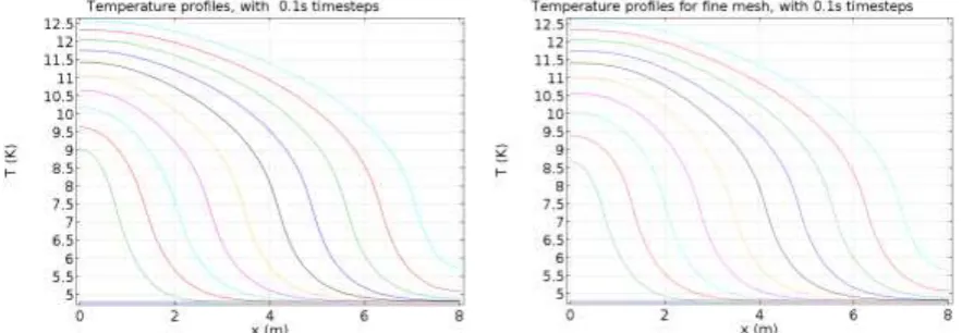
To verify the accuracy of the results obtained using this mesh, MQE and QPV results were compared to that of a simulation with an extremely fine mesh. Both meshes are partially shown in Figure 11. The optimized mesh for the comparison consists of 4512 elements, the extremely fine mesh consists of 551040 elements. The resulting temperature profile of both simulations can be seen in Figure 12. Each line depicts the temperature profile at a different time. The green line on the left is at t = 0.1, the next (red) one at t = 0.2, etc. It can be seen that the difference between the results is minimal. The corresponding MQE was unchanged and the QPV showed a difference of only 1%. Therefore it was concluded that the optimized, coarser mesh has an appropriate density.

Figure 11 (Part of) mesh for a single cable without insulation (left) and extremely fine mesh to compare results (right)

15

Results

Simulations were performed from 1 to 3 Tesla with corresponding currents for the B00 test coil’s ECT and BT sub-coils. Besides simulations for the full sub-coils, simulations of single conductors, both with and without insulation were performed. Similar to Figure 12, temperature profiles are shown in Figure 13 (left), this time for the full ECT sub-coil at 2T along with a that the normal zone

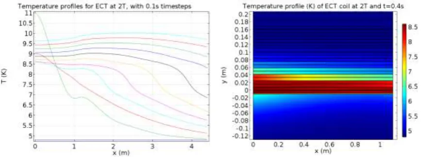
propagation accelerates. One can see how at first the heat pulse causes a local rise in temperature, after which the normal zone diffuses along the length of the conductor. The bump in the green line around x = 1.1 m indicates that the heat is also diffusing through the insulation to the next layer. Once the normal zone length exceeds the MPZ, the normal zone continues to propagate and the temperature profile at the edge of the normal zone becomes very similar at each successive time interval. Note that for a single cable simulation this propagation becomes a steady-state process. For a coil simulation however, the heat keeps building up in the layers of conductors that are already normal, adding more heat to the propagating normal front and causing it to accelerate as can be seen in Figure 13 (left). The QPV for the coil simulations is determined by dividing the distance covered by the moving normal front in one time step by the length of time of the step. The time step chosen for this determination is the one between the first and second temperature profile, after the first turn of the coil (1.1 m) has been passed, where the typical shape of the moving front is clearly visible and the critical temperature is exceeded (magenta and yellow line in this case). Note that for simulations below 1.5 T for the ECT conductor and at 1 T for the BT conductor, which corresponds to a current level of roughly 10 kA, the time steps were increased to 0.5 s for clarity. Figure 13 (right) shows the 2D temperature profile corresponding to the graph on the left at t = 0.4 s (magenta line). The continuity in temperature imposed by the periodic boundary conditions can clearly be observed.

Figure 13 1D Temperature profiles (left) and 2D temperature profile (right) of ECT coil at 2T

The current density and magnetic field of the propagating normal zone in a single ECT conductor without insulation at 1 T are shown in Figure 14. The front is moving from left to right. As mentioned before, the magnetic field is only used to describe the current in the conductor. The effect of the full magnetic field is taken into account in the material properties. It is visible in the figure that before the front has passed all the current runs through the superconducting core and that sometime after it has passed the current flows both through the core and stabilizer. It can be observed in Figure 14 as well that the length in x-direction along which current diffusion into the stabilizer takes place is over a meter long. For simulations at higher magnetic fields, this length increases to several meters, as the quench propagation velocity becomes many times higher. It is at and directly after the

16

Figure 14 Current density in a single ECT cable at 1T (left) as well as magnetic B-field (right)

Figure 15 Temperature plot (left) and current density (right) for a single cable that recovers after a heat pulse below the MQE was introduced

Figure 15 (left) shows 10 temperature profiles (t = 0 until t = 1) of a BT cable where the normal zone length did not exceed the MPZ, leading to recovery. The heat is spreading evenly through the conductor over time and no normal zone propagation occurs. Ascan be seen in Figure 15 (right), the current does not spread back evenly into the superconductor once the current sharing temperature has been exceeded, even though 15 seconds have passed and the temperature has decreased again. The current starts circulating around the edges of the core. This unusual current distribution results from the assumed infinite critical current density at 𝑇 < 𝑇𝑐𝑠, and the lack of cable twisting in the

model.

17

For the single cable simulations it can be seen that the MQE increases slightly when insulation is added and that the QPV decreases. This is due to the heat capacity of the insulation.

The MQE for the coil simulations is even higher than that of the insulated single cable simulations because there is more material for the heat to diffuse towards, away from the normal zone. The QPV however, is higher for the coil simulations than for the single cable simulations. This can be

explained by the heat already absorbed by unquenched conductor layers from quenched layers through the insulation, before the longitudinal quench propagation reaches this coil region, meaning these layers require less energy to turn to the normal state.

Figure 21 through Figure 24 show all the simulation results using aluminum stabilizer with RRR = 1100. Overall, the QPV is higher than that of the simulations using RRR = 3000 aluminum. This is to be expected because the higher resistivity results in more heat generation and the lower thermal conductivity lets less heat conducted away from the normal zone. The MQE is lower and can be explained with the same reasoning.

The effect of the thickness of the conductor on the QPV has also been simulated and results are shown in Figure 16. As is to be expected, the QPV decreases with cable thickness, because the extra aluminum creates a larger heat sink. This causes more heat to travel away from the propagating normal front, reducing its velocity. It is worth noting that at 4 times the cable thickness a 0.2 K temperature gradient between the core and the stabilizer surface, where the heat pulse is released, exists during the heat pulse. This also explains the why the slope of Figure 16 decreases; as the diffusion path between the core and extra stabilizer is becoming longer, it takes longer for the heat to diffuse. This reduces the effectiveness of the added stabilizer material. Furthermore the MQE is twice as large at 4 times the cable thickness than it is at the original thickness. This can be attributed to both the larger heat sink created by the aluminum stabilizer and the longer diffusion length for the heat to bridge between the stabilizer surface and the core.

Figure 16 Quench propagation velocity versus normalized cable thickness for an ECT cable with RRR = 3000 for the aluminum stabilizer

0 5 10 15 20 25

0 0,5 1 1,5 2 2,5 3 3,5 4 4,5

QPV

(m

/s

)

Normalized cable thickness

18

Figure 17 Computed quench propagation velocities for BT coil, cable with insulation and cable without insulation at different current levels compared to measured values [12] using aluminum with RRR = 3000

Figure 18 Computed minimum quench energies for BT coil, cable with insulation and cable without insulation at different current levels compared to measured values [12] using aluminum with RRR = 3000

0 5 10 15 20 25 30 35

0 5 10 15 20 25 30

QPV

(m

/s

)

Current (kA)

B00 BT quench propagation velocity, RRR = 3000

Measurements Coil Cable w. insulation Cable

1 10 100

0 5 10 15 20 25 30

MQE

(J

)

Current (kA)

B00 BT minimum quench energy, RRR = 3000

19

Figure 19 Computed quench propagation velocities for ECT coil, cable with insulation and cable without insulation at different current levels compared to measured values [12] using aluminum with RRR = 3000

Figure 20 Computed minimum quench energies for ECT coil, cable with insulation and cable without insulation at different current levels compared to measured values [12] using aluminum with RRR = 3000

0 5 10 15 20 25

0 5 10 15 20 25 30

QPV

(m

/s

)

Current (kA)

B00 ECT quench propagation velocity, RRR = 3000

Measurements Coil Cable w. insulation Cable

1 10 100

0 5 10 15 20 25 30

MQE

(J

)

Current (kA)

B00 ECT minimum quench energy, RRR = 3000

20

Figure 21 Computed quench propagation velocities for BT coil, cable with insulation and cable without insulation at different current levels compared to measured values [12] using aluminum with RRR = 1100

Figure 22 Computed minimum quench energies for BT coil, cable with insulation and cable without insulation at different current levels compared to measured values [12] using aluminum with RRR = 1100

0 5 10 15 20 25 30 35 40

0 5 10 15 20 25 30

QPV

(m

/s

)

Current (kA)

B00 BT quench propagation velocity, RRR = 1100

Measurements Coil Cable w. insulation Cable

0,1 1 10 100

0 5 10 15 20 25 30

MQE

(J

)

Current (kA)

B00 BT minimum quench energy, RRR = 1100

21

Figure 23 Computed quench propagation velocities for ECT coil, cable with insulation and cable without insulation at different current levels compared to measured values [12] using aluminum with RRR = 1100

Figure 24 Computed minimum quench energies for ECT coil, cable with insulation and cable without insulation at different current levels compared to measured values [12] using aluminum with RRR = 1100

0 5 10 15 20 25 30

0 5 10 15 20 25 30

QPV

(m

/s

)

Current (kA)

B00 ECT quench propagation velocity, RRR = 1100

Measurements Coil Cable w. insulation Cable

0,1 1 10 100

0 5 10 15 20 25 30

MQE

(J

)

Current (kA)

B00 ECT minimum quench energy, RRR = 1100

22

Discussion

For the coil simulations using RRR = 3000 aluminum, the MQE and QPV values that were computed were compared to the measurement data found in literature. The QPV simulation data shows the same general trend as the measurement data with respect to the current and above 17 kA shows a maximum error lower than 15%. The computed values for the MQE match the trend of the

measured values less well, but are within 50% above 20 kA, yielding an acceptable order estimation. For the ECT coil however, the minimum quench energies calculated below 20 kA are off. There are many parameters that can be (part of) the cause of this difference among which some are: the exact thickness of the ground insulation of the B00 coil is not known, the most inner turn for both the ECT and BT sub-coils where the heaters are located are slightly diagonal compared to the rest of the turns because they connect the two pancakes of each sub-coil and the RRR of the aluminum stabilizer is not known. It may also be possible that the measured MQE values at lower currents were affected by instability of the superconducting cable, by so-called flux jumps.

Because the normal zone propagation in a coil is not exactly steady-state because of the interaction between different layers of conductors, it is difficult to determine how to define the QPV of the coil simulations. The measurements from literature were performed by measuring how long it took for the normal zone to travel between two points that were at the most inner and outer turn of each sub-coil. This is not practical to try to accomplish in the current model because the heat capacity of the conductor leaving the coil after the most outer turn is not taken into account, nor is any heat transfer in the z-direction, resulting in too much heat inside the conductor in the simulation. It is however possible that the used method of determining the QPV in the model results in lower values than should be the case. On the other hand, in a real coil the contact area of each consecutive layer, starting from the inside, increases so that less heat is absorbed from the previous layer and more is lost to the next. Furthermore, magnetic field in real-life decreases with each turn, decreasing resistivity. This is not the case in the model. The computed QPV values are however close to the measured values from literature.

It can be seen from the results that for the BT coil simulations the MQE is relatively low and the QPV relatively high with respect to the measured values, compared to the ECT results. In the real B00 coil the current diffuses into the stabilizer in y and z-direction, in the simulations only in the y direction. This means that the current density in the model is slightly higher in the model. Because the virtual width c + d relative to the amount of stabilizer is considerably smaller for the BT conductor, it could be that the generated heat in the model is also relatively high, which would explain the difference. However, the difference in behavior between the BT and ECT models is small.

Conclusion

23

References

[1] G. Volpini, "Quench Propagation in 1-D and 2-D Models of High Current Superconductors," in

Proceedings of the COMSOL Conference 2009 Milan, Milan, 2009.

[2] M. Mentink, A. Dudarev, H. Pais da Silva, C. Berriaud, G. Rolando, R. Pots, B. Cure, A. Gaddi, V. Klyukhin, H. Gerwig, U. Wagner and H. ten Kate, "Design of a 56-GJ Twin Solenoid and Dipoles Detector Magnet System for the Future Circular Collider," IEEE Transactions on applied

superconductivity, vol. 26, no. 3, 2016.

[3] R. Ruber and A. Yamamoto, "Evolution of superconducting detector magnets," Nuclear

Instuments and Methods in Physics Research A, vol. 598, pp. 300-304, 2009.

[4] "CMS The Magnet Project Technical Design Report," CERN European laboratory for particle physics, Geneva, 1997.

[5] B. Cure, B. Blau, A. Herve, P. Riboni, S. Tavares and S. Sgobba, "Mechanical Properties of the CMS Conductor," IEEE Transactions on applied superconductivity, vol. 14, no. 2, pp. 530-533, 2004.

[6] S. Sgobba, D. Campi, B. Cure, P. El-Kallassi, P. Riboni and A. Yamamoto, "Toward an improved high strenghth, high RRR CMS conductor," IEEE Transactions on applied superconductivity, vol. 16, no. 2, pp. 521-524, 2006.

[7] A. Yamamoto, T. Taylor, Y. Makida and K. Tanaka, "Next Step in th Evolution of

Superconducting Detector Magnets," IEEE Transactions on applied superconductivity, vol. 18, no. 2, pp. 362-366, 2008.

[8] E. Boxman, M. Pellegatta, A. Dudarev and H. ten Kate, "Current Diffusion and Normal Zone Propagation Inside the Aluminum Stabilized Superconductor of ATLAS Model Coil," IEEE

transactions on applied superconductivity, vol. 13, no. 2, pp. 1684-1687, 2003.

[9] F. Juster, J. Lottin, L. Boldi, R. De Lorenzi, P. Fabbricatore, R. Musenich, D. Baynham and P. Sampson, "Stability of Al-stabilized Conductors for LHC Detector Magnets," IEEE transactions

on applied superconductivity, vol. 5, no. 2, pp. 377-380, 1995.

[10] A. Dudarev, E. Boxman, H. ten Kate, O. Anashkin, V. Keilin and V. Lysenko, "The B00 Model Coil in the ATLAS Magnet Test Facility," IEEE transactions on applied superconductivity, vol. 11, no. 1, pp. 1582-1585, 2001.

[11] Y. Iwasa, "Page 487 and appendix IV and V," in Case Studies in Superconducting Magnets,

Design and Operational Issues, Second Edition, New York, Springer, 2009, pp. 639-648.

[12] E. Boxman, A. Dudarev and H. ten Kate, "The Normal Zone Propagation in ATLAS B00 Model Coil," IEEE transactions on applied superconductivity, vol. 12, no. 1, pp. 1549-1552, 2002. [13] H. ten Kate, "The ATLAS superconducting magnet system at the Large Hadron Collider," Physica

24

[14] A. Woodcraft, "Predicting the thermal conductivity of aluminium alloys in the cryogenic to room temperature range," Cryogenics, vol. 45, no. 6, pp. 421-431, 2005.

[15] P. Desai, H. James and C. Ho, "Electrical Resistivity of Aluminum and Manganese," J. Phys. Ref.

Data, vol. 13, no. 4, pp. 1131-1172, 1984.

[16] J. Hust and A. Lankford, Thermal conductivity of aluminum, copper, iron and tungsten for temperatures from 1K to the melting point, Boulder, Colorado: National Bureau of Standards, U.S. Department of Commerce, 1984.

[17] F. Fickett, "Magnetoresistivity of copper and aluminum at cryogenic temperatures," Cryogenics Division, National Bureau of Standards, Boulder, Colorado, 1971.

[18] F. Fickett, "Magnetoresistance of Very Pure Polycrystalline Aluminum," Physical review B, vol. 3, no. 6, pp. 1941-1952, 1971.

[19] T. Amundsen and R. Sovik, "Measurements of the Thermal Magnetoresistance of Aluminum,"

Journal of Low Temperature Physics, vol. 2, no. 1, pp. 121-129, 1970.

[20] W. Nick and C. Schmidt, "Thermal magnetoresistance of copper matrix in compound

superconductors, a new measuring method," IEEE transactions on magnetics, vol. 17, no. 1, pp. 217-219, 1981.

[21] L. Bottura, "A practical fit for the critical surface of NbTi, LHC Project Report 358," European organization for nuclear research, Geneva, 1999.

[22] E. Marquardt, J. Le and R. Radebaugh, "Cryogenic material properties database," in 11th

25

Nomenclature

A Area (m2₎

B Magnetic field (T)

𝐵_𝑐2 Second critical magnetic field (T)

𝐵𝑐20 Second critical magnetic field at zero temperature (T)

𝐶_𝑝 Heat capacity (J/(kg∙K))

𝐶_{𝑐𝑜𝑟𝑒} Virtual width in z-direction of the model, a + b (m)

𝐼 Current (A)

𝐽 Current density (A/m2₎

𝐽_𝑜𝑝 Operating current density (A/m2₎

𝑘 Thermal conductivity (W/(m∙K))

𝐿 Length of cable in model (m)

𝑃 Power of heat pulse (J/s)

𝑅𝑡ℎ Thermal resistance (K/W)

𝑇 Temperature (K)

𝑇_𝑐 Critical temperature (K)

𝑇_𝑐0 Critical temperature at zero field (K)

𝑇𝑐𝑠 Current sharing temperature (K)

𝑇_𝑜𝑝 Operating temperature (K)

𝑇_𝑡 Transition temperature (K) ((𝑇𝑐𝑠+ 𝑇𝑐)/2))

t Time (s)

𝑡ℎ𝑐𝑎𝑏𝑙𝑒 Thickness of cable in model (m)

𝑡ℎ𝑐𝑜𝑟𝑒 Thickness of core in model (m)

𝑡ℎ_𝑖𝑛𝑠 Thickness of insulation in model (m)

𝜇₀ Permeability of vacuum (4π × 10−7 _H/m)

𝜌 Electrical resistivity (Ω∙m)

𝜌_𝑚 Density (kg/m3₎

FCC Future circular collider

LHC Large hadron collider

MPZ Minimum propagation zone

MQE Minimum quench energy

QPV Quench propagation velocity

26

Appendix A

B00 test coil BT:

24 kA operating current, 2.6 T peak field

Table 4 Simulation results for B00 test coil BT

B (T) I (kA) Tcs (K) Tc (K) PV (m/s) MQE (J)

1 9.23 8.02 8.82 1.7 90

1.25 11.54 7.82 8.72 3.7 50

1.5 13.85 7.63 8.63 5.3 29

1.75 16.15 7.44 8.53 7.7 19

2 18.46 7.26 8.43 10.8 13

2.25 20.77 7.07 8.33 15 7.0

2.5 23.08 6.88 8.23 19.3 4.0

2.75 25.38 6.68 8.13 24.5 1.8

3 27.69 6.48 8.03 29.8 1.3

B00 test coil ECT:

24 kA operating current, 2.9 T peak field

Table 5 Simulation results for B00 test coil ECT

B (T) I (kA) Tcs (K) Tc (K) PV (m/s) MQE (J)

1 8.28 8.18 8.82 1.5 80

1.25 10.35 8.02 8.72 2.5 55

1.5 12.42 7.86 8.63 4.2 30

1.75 14.48 7.70 8.53 5.8 20

2 16.55 7.54 8.43 8.4 14.2

2.25 18.62 7.38 8.33 10.8 10

2.5 20.69 7.22 8.23 14.6 6.0

2.75 22.76 7.06 8.13 18.6 3.0