For Review Only
Classification
Journal: Transactions on Image Processing
Manuscript ID TIP-18075-2017.R2
Manuscript Type: Regular Paper
Date Submitted by the Author: 10-Oct-2018
Complete List of Authors: Ding, Guiguang; Institute of Information System and Engineering, School of Software
Guo, Yuchen; Tsinghua University, Department of Automation Chen, Kai; Tsinghua University, School of Software
Chu, Chaoqun; Tsinghua University, School of Software Han, Jungong; Lancaster University
Dai, Qionghai; Tsinghua University, Department of Automation
EDICS:
2. SMR-SMD Statistical-Model Based Methods < Image & Video Sensing, Modeling, and Representation, 33. ARS-IIU Image and Video Interpretation and Understanding < Image and Video Analysis, Synthesis and Retrieval
For Review Only
DECODE: Deep Confidence Network for
Robust Image Classification
Guiguang Ding, Yuchen Guo, Kai Chen, Chaoqun Chu, Jungong Han, and Qiongai Dai
Abstract—The recent years have witnessed the success of deep
convolutional neural networks for image classification and many related tasks. It should be pointed out that the existing training strategies assume there is a clean dataset for model learning. In elaborately constructed benchmark datasets, deep network has yielded promising performance under the assumption. However, in real-world applications, it is burdensome and expensive to collect sufficient clean training samples. On the other hand, col-lecting noisy labeled samples is much economical and practical, especially with the rapidly increasing amount of visual data in the Web. Unfortunately, the accuracy of current deep models may drop dramatically even with 5% to 10% label noise. Therefore, enabling label noise resistant classification has become a crucial issue in the data driven deep learning approaches. In this paper, we propose a DEep COnfiDEnce network, DECODE, to address this issue. In particular, based on the distribution of mislabeled data, we adopt a confidence evaluation module which is able to determine the confidence that a sample is mislabeled. With the confidence, we further use a weighting strategy to assign different weights to different samples so that the model pays less attention to low confidence data which is more likely to be noise. In this way, the deep model is more robust to label noise. DECODE is designed to be general such that it can be easily combine with existing architectures. We conduct extensive experiments on several datasets and the results validate that DECODE can improve the accuracy of deep models trained with noisy data.
Index Terms—Deep Learning, Robustness, Confidence Model.
I. INTRODUCTION
I
MAGE classification has drawn considerable research in-terest from artificial intelligence, machine learning, and computer vision communities for several decades. It is funda-mental for object recognition [1], scene understanding [2], and many other important tasks [3–7]. After a long time with hand-crafted features [8, 9] and shallow models [10, 11], researchers have witnessed the dramatic progress in recent years benefiting from the development of deep convolutional neural networks (CNN) [12–15], which has led to beyond-human performance in many benchmarks, including object recognition benchmark ImageNet [1] and face recognition benchmark LFW [3]. By aGuiguang Ding, Kai Chen, and Chaoqun Chu are with the School of Software, Tsinghua University, Beijing 100084, China.
Yuchen Guo and Qionghai Dai are with the Department of Automation, Tsinghua University, Beijing 100084, China.
Jungong Han with the School of Computing and Communications at Lancaster University, Lancaster.
dinggg, [email protected], yuchen.w.guo, chenkai2010.9, cc-q1993, [email protected].
This work was supported by the National Key R&D Program of China (No. 2018YFC0806900), the National Natural Science Foundation of China (No. 61571269, 61327902), and the National Postdoctoral Program for Innovative Talents (No. BX20180172).
Corresponding author: Yuchen Guo.
Fig. 1: We use a keyword “dog” to retrieve images inGoogle
image search engine. Surprisingly, several non-dog images, like cat or background images, arise in the top-ranked results.
large number of local convolutions, nonlinear transformations, and complicated combinations, deep CNN is able to exploit the intrinsic characteristics of images and construct powerful semantic features from images as well as accurate classifiers. Generally, training a deep CNN model follows a standard supervised learning pipeline [16]. Firstly, a sufficiently large sample set with labels is collected, e.g., by expert labeling. Then, the labeled training set is fed into the model and an optimization algorithm is adopted, e.g., stochastic gradient descent, to tune the model parameters to minimize a kind of loss function, e.g., cross-entropy loss. However, it is easy to observe that a deep CNN model has a huge number of parameters, which is significantly more than previous shallow classification models. This property leads to a fact that training a deep CNN model requires much more training images than are needed for training shallow models. For example, a SVM classifier usually has hundreds to thousands of parameters, and hundreds of labeled samples can always result in good perfor-mance. On the contrary, a deep CNN model, like AlexNet [12] or DenseNet [15], may have millions of parameters such that it is highly probable for a deep CNN model to overfit a training set with only hundreds of images. In practice, a training set with at least tens of thousands of labeled images is required to train a deep CNN model especially when trained from scratch.
A. Motivation and Contribution
Due to the demand for a large number of labeled samples, how to collect a sufficient training set seems to be a critical issue for deep CNN model training. One may observe that the current training strategies simply assume that there is a relatively clean dataset available for model training, which is collected by, for example, expert labeling. This assumption 6
For Review Only
0 10 20 30 40 Noise ratio (%)
0 20 40
Error rate (%)
LeNet@MNIST
0 10 20 30 40 Noise ratio (%)
30 40 50 60
Error rate (%)
AlexNet@AwA
0 10 20 30 40 Noise ratio (%)
0 10 20 30
Error rate (%)
[image:3.595.58.545.109.230.2]DenseNet@CIFAR10
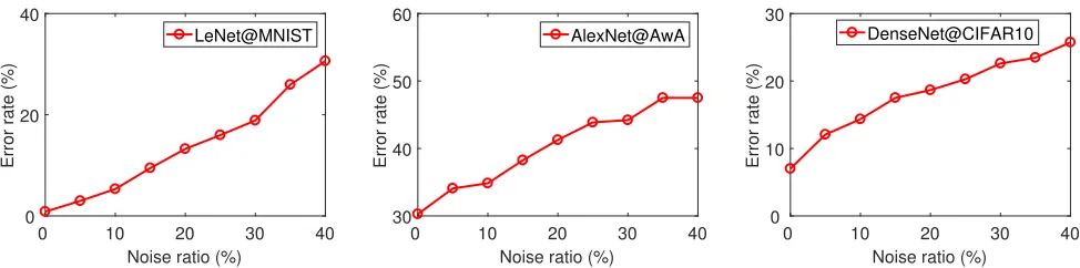
Fig. 2: The classification error rate of different models on different datasets with respect to different label noise ratios.
holds for many elaborately constructed benchmarks, like Ima-geNet. However, in practice, collecting such a large labeled training set is expensive and burdensome. For example, it may take millions of dollars to label an image dataset with ImageNet scale on Amazon Mturk platform. On the con-trary, collecting labeled samples from Internet, e.g., retrieving images from image search engine like Google using target keyword, turns out to be a convenient and economical way, which has drawn attention from some works [17, 18]. It can provide nearly labor-free labeled images with potentially unlimited size. Intuitively, the top-ranked images should be highly related to the target keyword so that they are always regarded as high-quality labeled images. Unfortunately, Web images are very noisy in practice. For example, as shown in Fig. 1, we use a keyword “dog” to retrieve images from
Google image search engine. In the top-ranked images,
there are several non-dog images, like cat images. When there are label noise, the performance of deep CNN models may drop dramatically. Empirically, we conduct experiments on MNIST [4], AwA [19] and CIFAR10 [20] datasets with LeNet [4], AlexNet [12] and DenseNet [15]. We add label noise to the training data by randomly mislabeling some images. The classification error rates on test set w.r.t. the noise ratio (the ratio between mislabeled images and all training images) are plotted in Fig. 2. Obviously, the error rate increases significantly with a little label noise. In some scenarios, even 5% to 10% label noise doubles the error rate. In addition, when performing recognition in complex background, the label noise also exists and has significant negative impact on the overall recognition accuracy [21–23].
The phenomenons above motivate us to develop robust deep CNN model training strategy to alleviate the negative influence of label noise in training data on the model so that it can work better in practical scenarios. In particular, we propose a deepconfidence network (DECODE) to address this issue. Specifically, by analyzing the data distribution of mislabeled images, we propose a simple yet effective confidence evalua-tion strategy to assign confidence score/weight to each sample. The purpose is to identify mislabeled images (i.e., noise) and assign small weights to them while assign large weights to confident ones. With the weighting strategy, the model will pay more attention to high-confidence samples, which are more likely to have correct labels, while it pays less attention to low-confidence samples, which are more likely to be mislabeled. To sum up, we make the following contributions in this paper:
1. We propose a novel framework, deep confidence network (DECODE), for robust image classification. It is capable of alleviating the adverse influence of noisy labels on training data in order to improve the accuracy of deep CNN models.
2. A simple yet effective confidence evaluation strategy is given based on the distribution of samples to identify noisy samples in training set. It produces a confidence score for each sample which reflects how likely the sample is mislabeled. Based on the confidence score, large training weights are assigned to high-confidence samples while small weights are given to low confidence ones. With this strategy, we can train deep CNN models with noisy data especially from scratch.
From the application perspective, DECODE has the follow-ing properties, makfollow-ing it practical in real-world applications:
3. DECODE is architecture independent such that it can be seamlessly combined with several popular CNN architectures, including LeNet, AlexNet, and the state-of-the-art DenseNet.
4. Experiments on several benchmark datasets and Web images demonstrate that DECODE can indeed improve the robustness of existing models, which verifies its effectiveness.
II. RELATEDWORK
Learning with noise is an important research topic in image classification and many related areas. This is a crucial issue especially for real-world applications because there is no guarantee that the training samples have perfectly clean labels. To address this issue, many approaches have been proposed, which can be roughly categorized into three main frameworks.
Noise robust algorithms.Many researchers notice that why the noisy samples significantly affect the model is because the model tries to “over-fit” the noise samples as they may contribute larger loss to the objective function than the normal samples. Therefore, one straightforward solution is to adopt noise-robust algorithms to train a model [6, 24–26], in which over-fitting avoidance techniques, such as regularization, are utilized to partially handle the label noise [27, 28]. In [25], Manwaniet al.investigated the robust learning problem in the empirical risk minimization framework. It theoretically ana-lyzed the robustness of different classification loss functions. Dietterich discussed the robustness of ensemble algorithm like bagging and boosting under label noise [29]. Abellan et al.
considered to improve the robustness of decision tress [30] with continuous features and missing data. However, these approaches mentioned above seem to be effective only when label noise can be managed by over-fitting avoidance [31]. 5
For Review Only
Bartlett et al. demonstrated that most of the loss functionsused by them are not completely robust to label noise [32].
Semi-supervised algorithms. Another popular strategy to handle label noise is semi-supervised learning. In this frame-work, extra supervision aiming at identifying mislabeled train-ing samples is utilized. In particular, another dataset with clean labels is constructed to assist the training with noisy labels under semi-supervised paradigm [33]. One widely-used approach is to use the combination of clean and noisy datasets to pre-train a model and then finetune it only with the clean set, where co-training and multi-view learning algorithms are often adopted. Veitet al.demonstrated that the above strategy did not fully leverage the information contained in the clean set. They proposed to use the pre-trained CNN model and the clean dataset to pre-process the noisy set and the both datasets were utilized to train a final model [34]. In addition, other semi-supervised techniques like label propagation are also utilized. For example, Chen et al. [35] proposed to use constrained bootstrapping and Fergus et al. [36] adopted a graph-based approach. They used a clean dataset to learn a feature representation and then constructed a mapping between noisy and clean annotations. However, they require a purely clean training set which is unavailable in many real-world scenarios. Furthermore, it seems quite difficult to incorporate their complicated strategies into the end-to-end CNN training.
Data relationship based algorithms. Many approaches attempt to explore the relationship in data, like image-image, image-label, label-label dependencies. Intuitively, the samples or labels are not independent to each other, whose relationship can be learned from data. Then based on the relationship, mislabeled samples are expected to be identified. Natarajan
et al. [37] and Sukhbaataret al.[38] proposed to explore the noisy label distribution and take it into consideration during model training. Xiaoet al.adopted an image-conditional noise model to capture the relationship between images and noisy labels. Veit et al. [34] proposed to capture the dependency of label noise from the input image, by learning a cleaning network about conditional dependency on image features. In addition, many other approaches attempted to identify the mislabeled samples by mining the relationship between data and then remove or correct them [39, 40]. However, these approaches get in trouble in distinguishing informative hard examples from harmful mislabeled ones. Some methods may remove too many suspicious samples and the over-cleaning could seriously reduce the performances of classifiers [31].
The above approaches mostly focus on training shallow models with noisy training data. Recently, how to train deep models with noise has drawn increasing interest. Wuet al.[41] proposed to incorporate a regularization terms with the model parameters to exploring the relationship between features and classes in order to address the noise in video frames. Reed
et al. [42] proposed a noise reconstruction method based on the data consistency using a bootstraping strategy, denoted as BOOTS. In their approach, a prediction is considered con-sistent if the same prediction is made given similar percepts. The noise distribution is modeled as a matrix mapping model and it is utilized to detect inconsistency and correct noisy labels. However, their approach assumes that there is explicit
mapping rules contained in label noise. Once the label noise is distributed randomly or has complicated patterns, their model may fail to construct the mapping matrix. Chen et al. [17] proposed to address the noise in a large dataset by another clean dataset as auxiliary supervision. However, their approach may fail when we train a model from scratch with no clean dataset, which is the main focus of this paper. Szegedy et al. [43] investigated the robustness of deep CNN model to adversarial samples. It is shown that even small noise in samples may lead to large misclassification rate. The effect of noisy training data is also considered in [44] and [45]. In summary, how to train a deep CNN model from scratch with only noisy training set is still an open and challenging issue.
Unsupervised algorithms. As surveyed in [46], there are many unsupervised algorithms for noise and outlier detection. However, these approaches are not feasible for our setting. In this paper and many related literatures, label noise instead of data noise is the focus. There is difference between them. For example, in AwA dataset for animal classification, label noise is that a tiger image is wrongly labeled as lion while data noise is that a non-animal image is included into the dataset. By unsupervised approaches, it is possible to identify the nonanimal images because they are outliers in the dataset which are far from all classes. However, a true tiger image will lie close to other tiger images, no matter what label it has. If it is wrongly labeled as lion, it will be an outlier for lion images, but not an outlier for the whole dataset because it is close to tiger images. In this case, it is difficult to be identified without label information in an unsupervised manner. In this paper, we care more about data that has wrong labels, instead of outliers of the dataset. As shown later, mislabeled samples lie close to normal data such that it is very difficult to detect them in a totally unsupervised manner. But with the class label, we can observe that some samples are outliers for their class.
DECODE is different from existing works in three perspec-tives. Firstly, the framework is different. There are many non-deep approaches for learning with noise. However, it is not clear how to combine them with deep networks, while DE-CODE itself is a deep learning framework. Compared to other deep approaches, we introduce a novel confidence evaluation module which is able to estimate the likelihood that a sample is mislabeled. The network can be trained in an end-to-end manner which can be combined with any existing deep CNN architectures. Secondly, the strategy is different. Some existing deep robust learning approaches require a clean dataset as auxiliary information to learn the true distribution of data. However, the clean dataset is sometimes very unavailable or expensive to construct. In this paper, we focus on learning from only one noisy dataset. For this setting, existing approaches mainly utilize the softmax output to identify the mislabeled data. However, softmax output is only reflects the probability that the sample belongs to each class. In each class, there are always many sub-classes where they may vary a lot from each other. Obviously, the softmax output is unable to well handle the intra-class diversity. DECODE, on the contrary, uses the fc output for analysis. The fc output is widely used as the image feature which can provide the relationship among images. Compared to softmax output, it provides much more 6
For Review Only
true class1true class2 false class1
(a) 5k iterations
true class1 true class2 false class1
(b) 10k iterations
true class1 true class2 false class1
(c) 50k iterations
true class1 true class2 false class1
[image:5.595.72.545.109.212.2](d) 200k iterations
Fig. 3: Visualization of features after different number of training iterations. We use CIFAR10 dataset and DenseNet. In these figures, “true class1” denotes samples having observed label “class1” and true label “class1”, and analogous to “true class2”. “false class1” denotes samples having observed label “class1” but true label “class2”, i.e., there are mislabeled and noise.
information, like the similarity between images and the cluster structure of data. In particular, DECODE adopts clustering hypothesis for noise identification. In addition, it assumes multiple clusters for each class, which is capable of handling the intra-class diversity and the sub-class structure for each class. Obviously, this strategy is more reasonable than the softmax based strategy. Moreover, Fig. 3 shows the behavior of deep networks during training with noise in practice, which lays solid foundation for DECODE. Thirdly, DECODE can be applied to more settings and applications. In fact, we can combine DECODE with any existing architectures, like LeNet, AlexNet and DenseNet. DECODE does not make any assumption about the noise distribution. Many other related approaches have some assumptions about the distribution. For example, BOOTS works well for conditional label permuta-tion, but fails in many other cases, like uniform permutation.
III. DEEPCONFIDENCENETWORK
A. Problem Definition and Notation
The problem is defined as follows. We are given a set of training data X = {xi|xi = {ri, li,˜li}}, where ri denotes the raw information of an image, like the RGB pixel values,
˜
li ∈ Lis the true label ofxi which is unknown for training, andli∈ Lis the observed label forxiwhich has a probability to be different from˜li. Our goal is to train a modelMusing the noisy training setX to predict the true label of a test image. Given a model and an input image, we denote the intermediary output (e.g., the output of a fully-connected layer) as fi.
In this paper, we consider uniform random label noise. Given an image xi, we have p(li = ˜li|xi) = ρ and p(li =
c|xi) = (1−ρ)/(C−1),∀c ∈ L\˜li, where C = |L| is the
number of classes in training set andρis the probability that the observed label is correct which is unknown for training.
B. Observation
First of all, it is worthy of investigating the behavior of label noise during training. We use CIFAR10 dataset and 40-layer DenseNet trained from scratch for illustration. We set the noise rate (nr= 1−ρ) to 0.1 and train the model with the noisy training set. We extract the output of the last pooling layer
(pool3), which is a 448-dimensional vector, as the feature
of each image. We use t-sne [47] to visualize the features. In particular, we randomly select two classes “class1” and
“class2”. The visualization is shown in Fig. 3. “true class1” denotes samples with correct label “class1”, and analogous to “true class2”. We care more about “false class1” denoting samples whose observed label is “class1” while true label is “class2”, i.e., they are mislabeled. Fig. 3 shows the trend of “false class1” samples with respect to different training iterations. We have one important observation from the result. There is an interesting phenomenon on “false class1”. At the beginning, e.g., after only5k or10k iterations, “false class1” samples perform more like the “true class2” samples than “true class1” samples. One possible and intuitive reason is that the model does not fit the data very hard at beginning and it only focuses on coarse characteristics of images to distinguish categories. In this scenario, it is difficult for the model to tell the difference of “false class1” and “true class2” because they actually have the same true labels given different observed labels. With further training, e.g., to200k iterations, the model is capable of finding the fine and tiny features to distinguish them such that “false class1” samples gradually move towards “true class1” samples. In fact, when a human is learning to distinguish different object categories, he/she will focus on coarse and general characteristics at first so that some outliers may be mis-recognized, and then the tiny detail is noticed [48]. Similar behavior of deep CNNs has been observed in [49] too. Their results suggest that deep networks tend to prioritize learning simple patterns first and then fit the abnormal data.
It takes a long procedure, instead of a one-step operation, for a deep CNN model to fit the label supervision from training set. This observation inspires us to involve a early stop strategy into the pipeline of model training. In particular, we propose to check the confidence of the model to a sample and assign small training weight to samples whose confidence is low. In fact, this strategy is somehow analogous to many semi-supervised learning (SSL) approaches [33]. In SSL, a model trained with some labeled samples is applied to a large number of unlabeled samples. Then the unlabeled samples with large confidence, e.g., measured by the maximum probability to a category p(c|x), are selected and treated as labeled samples to retrain the model because they are very likely to belong to the corresponding categories. With more training data and knowledge, the performance of this model can be improved in most cases. Our idea is similar to it but from the opposite view. We stop the training procedure in half way and then apply the obtained model to all labeled training samples. As suggested in 5
For Review Only
TrainingBatch
Training Batch
Training Batch
Training Batch
ܦܽݐܽଵ ݈ܾ݈ܽ݁ଵ ݓ݄݁݅݃ݐଵ
ܦܽݐܽଶ ݈ܾ݈ܽ݁ଶ ݓ݄݁݅݃ݐଶ
ܦܽݐܽଷ ݈ܾ݈ܽ݁ଷ ݓ݄݁݅݃ݐଷ
ܦܽݐܽସ ݈ܾ݈ܽ݁ସ ݓ݄݁݅݃ݐସ
ܦܽݐܽହ ݈ܾ݈ܽ݁ହ ݓ݄݁݅݃ݐହ
. . .
ܦܽݐܽ ݈ܾ݈ܽ݁ ݓ݄݁݅݃ݐ
. . .
. . .
. . .
...
conv. . .
. . .
fc softmax
݈ܾ݈ܽ݁
ݓ݄݁݅݃ݐ
confidence evaluation
ܦܽݐܽଵ ݎ݁݀ଵ ݂ܿ݊ଵ
ܦܽݐܽଶ ݎ݁݀ଶ ݂ܿ݊ଶ
[image:6.595.50.550.109.322.2]ܦܽݐܽଷ ݎ݁݀ ݂ܿ݊
ݓ݄݁݅݃ݐ
ൌ ݃ሺ݂ܿ݊
ሻ
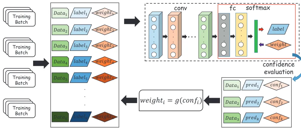
Fig. 4: The proposed DECODE for training deep CNN model with noisy labels. Conventional training strategy assigns the same weight to all samples. We find out that samples with noisy labels have different behavior from the ones with true labels during training. Based on this observation, we propose a confidence evaluation module to find the mislabeled samples and further assign different training weights to different samples. In this way, the influence of noisy samples is effectively suppressed.
Fig. 3, noisy/mislabeled samples tend to have low probability to their target labels because they should have other labels. Therefore, it is reasonable to assign smaller weights to them for subsequent training steps to suppress their influence so that the model can focus on samples which have true labels.
C. Framework and Approach
Based on the observation above, we propose DECODE for training deep CNN model with noisy data, whose framework is briefly illustrated in Fig 4. Previous training strategy assigns the same weight to all training samples. In this paper, we propose to give different weights for different samples, where the weight is determined by the confidence that it is correctly labeled based on the output of current model. A small weight is assigned to samples which are likely to have noisy labels. Then the weighted loss is backpropagated to tune model parameters. DECODE is architecture independent and we can combine it to any deep CNN architectures. In fact, existing architectures mostly follow a convolution-fully connected (fc) style which has a large number of convolution layers (together with activation and pooling layers) at first and a few fully connected layers at last. In this work, we adopt the output of the last layer before the classification layer as fi for a sample xi, like the
pool3layer in DenseNet andfc7 layer in AlexNet.
Now we compute the confidence of each training sample. Confidence evaluation is based on the clustering hypothesis1 which is also demonstrated in Fig. 3. Clustering hypothesis as-sumes that data from the same class should form a cluster and be similar to each other, which is a fundamental assumption for many machine learning techniques, including semi-supervised learning [33]. In DECODE, we also utilize this hypothesis. In particular, for each class c ∈ L, we have a set of clustering
1https://en.wikipedia.org/wiki/Cluster hypothesis
centerskc
j for it, whose number is Kc. In this simplest case, we use1cluster center for each class. However, in real-world scenarios, the class structure is more complicated. Therefore, it seems more reasonable to assume multiple cluster centers for each class. Then we introduce a violation factor as below:
v(xi) =
X
c∈L
Kc
X
j=1
f(max(0, d(fi, kjli(xi))−d(fi, k
c
j) +λ)) (1)
Here,d(·,·)is a distance measure, like Euclidean distance and cosine distance.λis a non-negative margin parameter.j(xi) = argminjd(fi, klji). We care about the abnormal samples which violate the clustering hypothesis, i.e., its distance to its own class’ center is larger than to other classes’ centers.f(x)is a counter function which counts the times of violations. It can be hard count wheref(x) = 1ifxis true or 0 otherwise, or soft countf(x) =xwhich considers the degree of violation. Obviously, the larger v(xi) is, the more likely xi is to be mislabeled because it is closer to many other classes’ centers instead of its own observed label’s center. One may say that there is a very simple strategy by considering the softmax outputpiof a sample. However, our strategy in Eq. (1) has one advantage over this strategy. Eq. (1) considers the distribution structure of training data while softmax based one considers the information of a single sample only. Therefore, Eq. (1) uses more information such that its prediction is more reliable.
Based on the violation factor, it is straightforward to define the confidence which is a monotonically decreasing function of the violation factor. In this paper, we adopt a simple function which simultaneously normalize the value to[0,1]as below:
confi=exp(−αv(xi)) (2)
where αis a factor to control the decay rate. Then, we can compute training weight wi using confi. As confi has been 6
For Review Only
Algorithm 1 Training DECODEInput: Training dataX, model structures, parameters;
Output: A deep CNN model; 1: Randomly initialize the model;
2: Runk-means clustering on image features for each class to get the initial cluster centerskc
j;
3: repeat
4: Select a training batchB;
5: ForwardBthrough the model and get image featuref; 6: Compute violation factorv(xi)using fi by Eq. (1);
7: Computeconfi and training weightwi by Eq. (2);
8: Compute the weighted loss by Eq. (3); 9: Back-propagate the weighted loss by SGD; 10: Update centerskc
j by Eq. (4);
11: untilConvergence or maximum iterations; 12: Return the obtained model;
normalized, we simply setwi =confi. Given a training batch
B ={xi|i= 1, ..., b}, the weighted loss is defined as below:
Loss(B, ϕ) =
b
X
i=1
wiloss(xi, li, ϕ) (3)
whereϕis the current model andlossis a loss function like cross entropy. With a training weight, the influence of noise can be effectively suppressed so that the model is more robust. The learning algorithm now consists of two parts, training deep network and training confidence evaluation module. When training a deep network, we can use stochastic gradient descent to minimize Eq. (3) just like the usual way. This can be done easily based on existing deep learning tolls, likeCaffe2. Then we need to update the confidence evaluation module. In particular, we need to update cluster centers kc
j. Inspired by [50], these centers can be also updated by gradient descent. Specifically, in each training batch, centerkc
j is updated as:
kc
j=k
c
j−τ
Pb
i=1δ(j(xi) =j∧li=c)wi∂d(fi, k
c
j)/∂kcj
1 +Pbi=1δ(j(xi) =j∧li=c)
(4)
where τ is a tiny step size andδ(z) is an indicator function which is 1 if z is true or0 otherwise. Here we also take the weightwiinto consideration so that the centers focus more on reliable samples. Here∂d(fi, kcj)/∂kjc is the partial derivative of the distance measure to kc
j. In this paper, we consider the Euclidean distance. We can utilize other distance or similarity measures also, like cosine and inner-produce similarity. We empirically find out that Euclidean distance is slightly better. We summarize the training algorithm of DECODE in Al-gorithm 1. It basically follows the mini-batch based iterative procedure for training a deep CNN model. The main difference lies in line 6 to line9 where we evaluate the confidence of a sample and assign a training weight based on its confidence so that the influence of mislabeled samples is suppressed. The confidence evaluation module is updated adaptively in line10. Based on the training algorithm above, the obtained deep CNN model shows more robustness to label noise in training data.
[image:7.595.339.534.122.173.2]2https://github.com/BVLC/caffe
TABLE I: Description of benchmark datasets
Dataset #classes #training #test MNIST 10 60,000 10,000
AwA 50 24,380 6,095
CIFAR10 10 50,000 10,000
As shown in Algorithm 1, training DECODE requires just a few extra operations than the standard back-propagation based deep model training, which includes computing the violation factor, confidence, and the training weight. These operations only need some simple vector operations, of which the computational cost is much less than the cost of the forward and backward propagation in the convolution layers. Therefore, the training speed is comparable to training in the original way. Based on the Caffe toolbox, training an AlexNet can be done in a few hours using one GPU.
IV. EXPERIMENT
A. Data Preparation
In our empirical studies, we select three different benchmark datasets which have different size, complexity, and topics.
MNIST[4]. MNIST dataset is a handwritten digits dataset. It consists of 70,000handwritten images representing a digit from “0” to “9” where60,000images are used as training set and the other 10,000are test set. Each image has a size of
28×28and each pixel is represented by its gray-scale value.
Animals with Attributes (AwA)[19]. AwA dataset is build for recognizing animal images in the wild. It has 50 animal species together with30,475images. We randomly split80%
images as training set and the remaining20%images as test set. Because the images are captured in the wild, they have various and noisy background, and the animals show different poses. Therefore, this dataset is complicated to some extent.
CIFAR10 [20]. CIFAR10 dataset is a popular dataset for image classification task. It has 10 common objects like “truck” and “cat” where each object has 6,000 image. We follow the standard split where50,000images are utilized for training and the other10,000images are used for evaluation.
B. Deep CNN Models
We consider three deep CNN models. The first is LeNet [4] which is a very simple deep CNN model published about twenty years ago, which is one of the earliest deep CNN models. LeNet is mainly for simple datasets like MNIST. The second is AlexNet [12] published in 2012. It is one of the most well-known models. It achieved great success in ImageNet challenge and attracted considerable attention from both academia and industry. The third is DenseNet [15] which is one of the state-of-the-art networks currently. In this paper, we consider the40-layer (k= 12) network. DenseNet is the most complicated and has the best performance. There are also many other network structures, such as VGG [13] and ResNet [14]. But they have similar complexity and perfor-mance with the selected structures in our experiment. Hence we do not use them all but some representative ones. In fact, the proposed DECODE framework can be combined with them all since network structure itself is not the focus of this paper. 5
For Review Only
TABLE II: The classification error rate comparison on different datasets with different models. LeNet@MNIST AlexNet@AwA AlexNet@CIFAR10 DenseNet@CIFAR10 Noise Rate Original DECODE Original DECODE Original DECODE Original DECODE
0% 0.85% 1.48% 30.27% 30.14% 9.56% 8.80% 7.00% 6.60%
5% 2.97% 1.51% 34.08% 32.86% 10.75% 9.89% 12.07% 8.84%
10% 5.32% 1.53% 34.84% 34.74% 11.01% 9.93% 14.33% 10.90%
15% 9.46% 1.70% 38.26% 36.05% 11.69% 10.01% 17.51% 11.44%
20% 13.25% 1.73% 41.27% 37.71% 11.82% 10.92% 18.66% 12.51%
25% 15.58% 1.81% 43.87% 37.36% 12.83% 11.28% 20.27% 13.71%
30% 18.88% 1.84% 44.21% 37.44% 12.91% 11.35% 22.61% 14.02%
35% 25.95% 2.60% 47.51% 39.47% 13.45% 12.28% 23.46% 15.00%
40% 30.62% 2.77% 47.50% 39.09% 14.08% 12.62% 25.74% 15.62%
C. Experiment Settings
We evaluate our framework for image classification task. The classification error rate on test set is used as the metric:
Error Rate=
Pnt
i=1I(pi 6= ˜li)
nt
(5)
wherentis the number of test samples,˜liis the true label ofi -th sample andpiis the predicted label by the model, andI(x) is an indicator function which is1ifxis true or0otherwise. Our goal is to evaluate models trained with noisy data. But we should notice that the benchmark datasets are almost noiseless. So we manually add label noise to them. In par-ticular, we set a noise rate nr. Then given a training sample with label ˜li, its observed labelli which is actually used for training is sampled with probability p(li= ˜li) = 1−nrand
p(li = c) = nr/(C−1),∀c ∈ L\˜li where C = |L|. We change the value of nr in 0.05 : 0.05 : 0.4 and construct a new noisy training set. A deep CNN model is trained by the new training set and is evaluated on the test set. In this way, we can comprehensively evaluate the robustness of models.
D. Implementation Details
To implement DECODE, we use Caffe toolbox. For all cases, we set the base learning rate as1e-4and weight decay as 5e-5. The batch size is 128. For MNIST, the maximum iteration is 30k. For AwA and CIFAR10, we train DECODE for300k. If we use a pre-trained model for initialization, it may contain noiseless knowledge from other dataset. So we train all models from scratch. Because we use random initialization, the featuresfiproduced at the beginning have very low quality so that the confidence evaluation is not reliable since the cluster structure is not significant after random initialization. As observed in Figure 3, the noise data has little influence on training at very beginning because the model tries to capture general knowledge applicable for most data. So we train networks without the confidence evaluation for the first
1k iterations by assigning the same weight1to all samples.
E. Effectiveness Verification
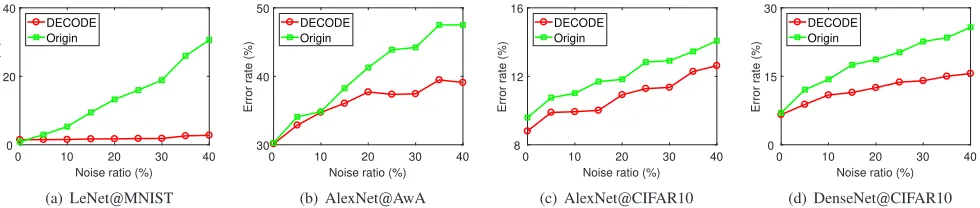
We firstly verify the effectiveness of DECODE. We change the noise rate and evaluate the classification error on test set for each method. The comparison between the original model and DECODE is summarized in Table II and the trends are plotted
in Figure 5. It can be observed that the performance of LeNet, AlexNet, and DenseNet drops dramatically with more noise while DECODE shows more robustness. Therefore, DECODE consistently and significantly outperforms the original ones. Besides, we have the following observations from the results. Firstly, LeNet@MNIST raises error rate by 29.77%when we increase the noise rate from 0 to 40%, AlexNet@AwA raises by 17.23%, AlexNet@CIFAR10 raises by4.52%, and DenseNet@CIFAR raises by 18.74%. On the other hand, with the proposed DECODE, the error rates are raised by
1.29%,8.95%,3.82%, and9.02%respectively, relatively sup-pressing the influence of noise by 95.67%, 48.06%,15.49%
and 51.87% compared to the original models. The results demonstrate that DECODE can indeed improve the robustness of existing models, which is the motivation of this paper.
Secondly, we can observe that DECODE has slightly bet-ter performance for AlexNet@AwA, AlexNet@CIFAR, and DenseNet@CIFAR when the noise ratio is0. When nr= 0, there is no extra manual noise in the datasets. In this case, we use the original datasets. Since these datasets were elaborately collected, we can regard them as “clean” datasets. One pos-sible reason is that the original datasets may contain noise to some extent. DECODE is capable of addressing the noise and leads to better performance. One may argue that the examples close to the boundary is informative. But we should notice that they are more likely to be mislabeled in practice since they are more ambiguous. From one side, if a model pays more attention to them, it can obtain important knowledge to distinguish two classes if these examples are correctly labeled. However, on the other side, if they are mislabeled, paying more attention to them leads to a worse model since it is misled. In DECODE, samples close to boundary are paid less attention to so that the noise in them has less impact on the model. In addition, doing so can also make the model focus more on the general knowledge of a class, which makes it generalize better on test data. In MNIST, the data is quite simple and we can regard it as a purely clean dataset. So the examples close to boundary provide useful information. DECODE down-weight them so that it performs slightly worse than the original model. However, when there is only 5% noise, the performance of original model drops significantly while DECODE does not. AwA and CIFAR10 are collected from real world and they are more complicated than MNIST. Therefore, they naturally contain label noise themselves. In this situation, paying more 6
For Review Only
0 10 20 30 40 Noise ratio (%) 0
20 40
Error rate (%)
DECODE Origin
(a) LeNet@MNIST
0 10 20 30 40 Noise ratio (%) 30
40 50
Error rate (%)
DECODE Origin
(b) AlexNet@AwA
0 10 20 30 40 Noise ratio (%) 8
12 16
Error rate (%)
DECODE Origin
(c) AlexNet@CIFAR10
0 10 20 30 40 Noise ratio (%) 0
15 30
Error rate (%)
DECODE Origin
[image:9.595.61.551.109.213.2](d) DenseNet@CIFAR10 Fig. 5: The classification error rate comparison on different datasets with different models.
attention to examples close to boundary is likely to mislead the model and thus DECODE has better performance. In fact, in practical applications, when the model is trained by a training set collected from real world for a complicated task, like a fine-grained classification task, it is almost impossible to ensure that the training set is as clean as MNIST. The results demonstrate that DECODE can perform well in practice.
Thirdly, on CIFAR10 dataset, noise has less impact on AlexNet than DenseNet. In fact, DenseNet is one of the most state-of-the-art architectures and it is able to discover more knowledge and details from training data, and that is why DenseNet performs better when there is 0% noisy data. As discussed above, a network progressively fit the data where general knowledge is firstly captured and specific details later. For DenseNet, the noisy information is “over-fitted” because DenseNet is complicated enough so that the model is heavily influenced. On the other hand, AlexNet is relatively simpler than DenseNet such that it is not able to finely capture the distribution of noise. In this case, AlexNet seems more robust to noise data and thus performs better. With DECODE, the performance drop of DenseNet is effectively suppressed.
Fourthly, LeNet@MNIST has the largest performance drop among all settings. In fact, MNIST is the easiest dataset in our experiment and the intra-class variance is relatively small. Therefore, it is easy to capture the information of training data, even if we use a simple network like LeNet. In this way, the network will try to fit noisy data during training and get significantly affected. On the other hand, DECODE utilizes the cluster structure to evaluate the confidence of each training sample. The small intra-class variance makes it easier to identify the outliers and assign very small weights to them. Because the dataset is easy, DECODE achieves only 2.77%
error rate even with 40%mislabeled images in training data. Fifthly, the results demonstrate of the superiority of image features from the fc layer to the softmax output for confidence evaluation. Using the softmax output to identify mislabeled samples is exactly the method in our baseline BOOTS. It adopts the inconsistency of softmax output as the metric. By a bootstrapping framework, it pays less attention to inconsistent labels. By doing so, it attempts to develop more robust models. However, it has strong assumption to the noise distribution. It mainly focuses on conditional label permutation. There-fore, it performs observably worse in the experiments where uniform noise is adopted. In addition, softmax output only shows the probability relationship between data. It ignores the complicated multi-cluster structures. For example, even
for class “dog”, there are some sub-classes of “dog” which have significant appearance difference to each other, like “Labrador” and “Chiwawa”. The softmax output is not able to reflect the difference. In DECODE, we base our framework on clustering hypothesis and several clusters are used for each class. In this way, the intra-class diversity is well addressed. Identifying mislabeled data is analogous to detecting abnormal samples for a class. Well capturing the intra-class diversity can help to achieve this goal and lead to more robust models. We notice that some works attempt to calibrate the softmax output [51] in order to make deep networks more accurate. Unfortunately, calibrating softmax fails to address the noisy labels because it is not capable of handling the complicated multi-cluster structures in real-world image datasets.
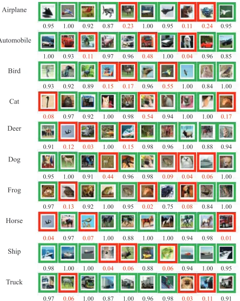
Finally, to better verify the effectiveness of DECODE, we show some exemplar images in Fig. 6. In particular, we use DenseNet@CIFAR10 in this experiment and set noise ratio to
30%. The training weights obtained by Eq. (1) and (2) after
50k iterations are given. Generally, the noisy samples which are mislabeled have very small training weights (e.g.,<0.2) while the correct samples have large weights (e.g.,>0.8). This phenomenon clearly demonstrates that DECODE can indeed identify noisy samples and suppress their influence by assign-ing small weights to them while capturassign-ing the knowledge in correct training samples by assigning large weights to them.
F. Comparison to Other Approaches
Besides DECODE, there are some approaches focusing on training deep CNN with noisy labels. We consider two state-of-the-art approaches in this section. The first work is [18] which uses an extra layer to match the noisy label distribution, denoted as NLD. The second work is [42] which employs bootstrapping to address the noisy samples, denoted as BOOTS. Although there are many approaches discussed in Section II working on learning with noise, they mostly focus on non-deep approaches. It is not clear how to combine them with deep CNN training. We still consider one baseline [52], termed as IR, in the comparison. However, it is a shallow approach which cannot be trained in an end-to-end manner in deep networks. Therefore, we use a pretrained AlexNet on ImageNet as the feature extractor for AwA and CIFAR. This approach takes the features from the pretrained deep model as input and trains a series of one-vs-all binary classifiers for each class. For MNIST, we use the raw pixel gray values as image features. It should be noticed that it needs the noise rate as side information, for which the true noise rate is adopted. 5
For Review Only
Airplane
Automobile
Bird
Cat
Deer
Dog
Frog
Horse
Ship
Truck
0.95
1.00
0.92
0.87
0.23
1.00
0.95
0.11
0.24
0.95
1.00
0.93
0.11
0.97
0.96
0.48
1.00
0.04
0.96
0.85
0.93
0.92
0.89
0.15
0.17
0.96
0.55
1.00
0.84
1.00
0.08
0.97
0.92
1.00
0.98
0.54
0.94
1.00
1.00
0.17
0.91
0.12
0.03
1.00
0.15
0.98
0.96
1.00
0.88
0.94
0.95
1.00
0.91
0.44
0.96
0.98
0.09
0.04
0.06
1.00
0.97
0.13
0.92
1.00
0.95
0.02
0.75
0.08
0.84
1.00
0.04
0.97
0.07
1.00
0.88
1.00
1.00
0.94
0.98
0.01
0.98
1.00
1.00
0.04
0.06
0.88
0.06
0.94
1.00
0.95
[image:10.595.68.561.105.722.2]0.97
0.06
1.00
0.87
1.00
0.96
0.98
0.03
0.11
0.91
Fig. 6: Exemplars of confidence evaluation and sample weighting. We use DenseNet@CIFAR10 for demonstration. We set noise ratio to30%and train DenseNet with DECODE. We show the training weight obtained by Eq. (1) and (2) after training for50k iterations. The texts on the left denote the true class labels. The images with green boxes are with the correct labels while the ones with red boxes are with the wrong labels. DECODE can effectively identify mislabeled (noisy) samples and assign very small weight to them to suppress their influence. On the other hand, correct samples always have large weight. 6
For Review Only
0 10 20 30 40 Noise ratio (%)
0 20 40
Error rate (%)
DECODE BOOTS NLD IR Origin
(a) LeNet@MNIST
0 10 20 30 40 Noise ratio (%)
30 40 50
Error rate (%)
DECODE BOOTS NLD IR Origin
(b) AlexNet@AwA
0 10 20 30 40 Noise ratio (%)
5 15 25
Error rate (%)
DECODE BOOTS NDL IR Origin
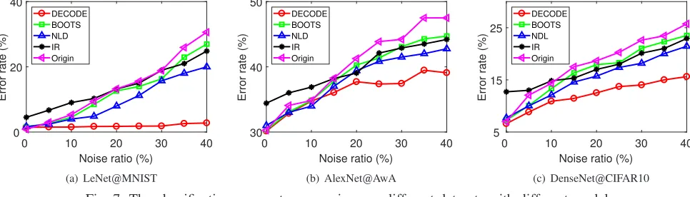
[image:11.595.60.543.114.252.2](c) DenseNet@CIFAR10 Fig. 7: The classification error rate comparison on different datasets with different models.
Sports Artifacts Datasets 10
20 30 40 50 60
Accuracy (%)
Origin BOOTS NLD DECODE
(a) Comparison on YFCC
0 10 35
Noise ratio (%) 10
15 20 25 30
Error rate (%)
ILCC OMP AlexNet DECODE
(b) Transferability study. AwA to CIFAR10
0 10 35
Noise ratio (%) 20
30 40 50 60
Error rate (%)
AlexNet BOOTS NLD DECODE
(c) Structured noise. AlexNet@AwA Fig. 8: More investigation on robust image classification.
Here we consider LeNet@MNIST, AlexNet@AwA and DenseNet@CIFAR10. The classification error rates under d-ifferent noise rates for all approaches are plotted in Fig. 7. Generally, these approaches have better performance than the original ones, especially when there is large noise rate, e.g.,
40%. DECODE significantly outperforms the other two ap-proaches, which demonstrates its superiority for robust image classification. We can observe BOOTS is only slightly better than the original models. This is because BOOTS mainly focuses on conditional label permutation. For example, a “dog” image may be mislabeled as “cat” but not “truck”. In our experiments we use uniform label noise so that they cannot well handle this situation. In fact, because the confidence evaluation in DECODE is based on the cluster structure of images, it is more general than BOOTS and capable of han-dling more kinds of label permutations. NLD is more flexible about how the noise is generated and thus it is much better than BOOTS. However, NLD relies heavily on the estimation of the distribution of noise, which is a quite challenging task. In fact, it seems the estimation of NLD is not accurate enough in many cases. On the other hand, DECODE addresses the noise from the data perspective and makes use of the data distribution to estimate the probability that a sample is mislabeled, which seems more reliable and accurate from the experiment results.
G. Comparison on YFCC100M
To better verify the efficacy of DECODE, we adopt an-other large-scale real-world benchmark dataset Yahoo Flickr Creative Commons 100 Million (YFCC100M)[53], which is an ideal benchmark for learning from noise. In particular, we
use the “Sports”, “Artifacts” subsets, which have238and323
classes, as well as 150k and 170k images respectively. For each subset, we use70%examples as the training set and the remaining30%examples as the test set. Since these datasets have many classes, we follow [54] and adopt mean average precision (mAP) as the evaluation metric. Since we focus on the methodology of learning from noisy labels rather than squeezing the performance numbers, we still utilize AlextNet as the basic model for our evaluation. For these datasets, we train DECODE for500k iterations. The other training details are the same as the ones introduced in Section IV.D.
The comparison is shown in Fig. 8(a). From the results we can observe that DECODE consistently and significantly out-performs the other baseline approaches, which demonstrates the effectiveness of DECODE for large-scale noisy datasets.
H. More Results
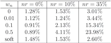
It is interesting to investigate how to deal with the low-confidence samples. In the above experiments, we use soft weight given by Eq. (2). In fact we can use hard weight. For example, we can set a threshold τ and assign weight 1 to samples of which the confidence is larger thanτ and weight
wnto the ones of which the confidence is smaller thanτ. Here we use LeNet@MNIST for analysis. We change the value of
τ in [0.05 : 0.05 : 0.3] and report the best results for hard
weight. We summarize the comparison between hard weight with differentwn and soft weight in Table III. Generally, as
nr increases, assigning smaller weights (e.g., 0.01) leads to better result and directly removing the suspicious samples (i.e.,
wn= 0) can result in good performance. Soft assign performs 5
For Review Only
TABLE III: The effect of weighting strategieswn nr= 0% nr= 10% nr= 35%
0 1.28% 1.53% 3.01%
0.01 1.12% 1.24% 3.44%
0.1 0.91% 2.13% 15.34%
0.5 0.89% 4.11% 23.98%
soft 1.48% 1.53% 2.60%
a little worse than wn= 0.01 whennr= 0%andnr= 10% because soft assign not only changes the weight of suspicious samples, but also has moderate impact on normal samples. In this case, the knowledge in normal data is likely to be under-explored. But we need to point out that hard assign needs another hyper-parameter τ which is difficult to set because we are unaware of the noise ratio and the properties of image features in advance. Therefore, using the soft assign strategy seems more reasonable and practical in real-world scenarios.
In addition, learning transferable features is an important task for deep networks. After pretraining, the transferable features can be used for other tasks, like detection [55], retrieval [56], and tracking [57]. In this part, we investigate the transferability of the deep networks trained with noise data. In particular, since AwA has more classes than CIFAR10, we pretrain a deep model by AwA with noise. Then we use the last fc layers output as image feature for CIFAR data, which is a 4,096-dimensional vector for AlexNet. We use AlexNet as the model and train it on AwA by the settings introduced in Section IV.D. Then the image features are extracted for CIFAR10. A linear SVM classifier is employed as classifier. When training the SVM, we set the parameterC= 1 consis-tently in all experiments. We adopt libLinear3toolbox. We use the original AlexNet and the DECODE version. Besides, we also consider two non-deep approaches as baseline [58, 59]. CIFAR10 is noiseless and we only change thenr for AwA.
The results are summarized in Fig. 8(b). It can be observed that deep based features yield better results than the non-deep ones in most cases. More importantly, DECODE shows better performance than the original AlexNet. When the nr
keeps increasing, AlexNet has observable performance drop while DECODE’s drop is much smaller. The results above indicate that DECODE is capable of generating transferable features, even trained by noisy data. In addition, as introduced in the algorithm, the uncertain and difficult samples which require detailed information to distinguish are down weighted so that the deep network can pay more attention to the general knowledge of a class, making it generalize better on test data. We also consider to pretrain a model on a noisy source dataset (e.g., AwA with 35%noisy labels) and then finetune it on a target dataset(e.g., CIFAR10). We find out that if the target dataset is clean, the finetuned DECODE is only marginally better than the original AlexNet because the clean dataset may correct the wrong knowledge in the pretrained models. On the other hand, if the target dataset is noisy, the results are very similar to the ones in TABLE II. This observation is consistent with [60]. They also notice that
3http://www.csie.ntu.edu.tw/∽cjlin/liblinear/
0
10
50
100
500
#Clean samples
0
20
40
60
80
Accuracy (%)
Origin Origin+Web DECODE+Web
Fig. 9: The performance by training with Web images.
pretraining on a noisy dataset has less influence if it is then finetuned on a clean dataset than directly using the features.
Furthermore, we use uniform random noise in the ex-periments above. One may care about the structured label noise. With structured noise, the probability that one image is mislabeled as a wrong class varies for different classes. For example, a “dog” image is more likely to be mislabeled as “wolf” than “fish” because it is more similar to the former. In this part we investigate the performance under structured noise. In particular, we use AwA dataset. AwA dataset has an attribute vector for each class which is an85-dimensional binary vector describing the attributes like the color of an animal category. The similarity between two classes attribute vectors can reflect the relationship between them. If two classes have similar attributes, they have many properties in common. Based on the attribute similarity, we can define the structured noise. Specifically, it is reasonable to assume that two similar classes are more likely to be mislabeled to the other. We generate the structured label noise as follows based on the attribute/class similarity. Suppose the cosine similarity between class A and B is cos(A, B)4. We define the probability that an image in A is mislabeled as B to be
nr∗cos(A, B)/Z, wherenris the pre-defined noise ratio (like
5%), andZ =PC6=Acos(A, C)is a normalized factor. With the probability, the training images are randomly mislabeled. We still use AlexNet here. The comparison is shown in Fig. 8(c). It can be observed that the overall performance with structured label noise is slightly worse than the uniform noise. This is reasonable because the mislabeled data from similar classes is more difficult to identify. But DECODE still has much better performance than the original model, which indicates that DECODE can well address the structured noise.
I. Training with Web Images
Collecting a large number of clean training images is expensive. On the other hand, retrieving labeled images from Web is almost free. In some cases, we can use Web images to help the target task. The Web images are noisy as shown in
4Since the attribute vectors in the dataset have 0/1 binary elements, the
cosine similarity between two attribute vectors is definitely non-negative.
[image:12.595.80.269.122.196.2]For Review Only
Fig. 1, which indicates that adopting a robust model trainingapproach is necessary. Now, we investigate the performance of DECODE for training with Web images. In particular, we use AlexNet@CIFAR10 because AlexNet seems more robust in this case. We use the class name in CIFAR10 as keywords to retrieve images in Google Image search engine and the firstly returned images are used as labeled training data. We also use a small number of clean samples in CIFAR10 for training.
We add5,000Web images (500per class) into training data and we change the number of clean samples per class from0to
500. We compare the original model with only clean training data, the original model with both clean and Web data, and DECODE with both clean and Web data. The comparison is summarized in Fig. 9. Obviously, incorporating Web images can significantly improve the performance, especially there are only a few clean samples like 10 or 50, although Web images are noisy. By using DECODE, the accuracy is further improved. When the Web images dominate the training set, e.g., there are less than 100 clean images per class, the improvement given by DECODE is more significant. This comparison clearly demonstrates that DECODE can indeed suppress the impact of noise and explore valuable knowledge.
V. CONCLUSION
In this paper, we investigate training deep CNN models with noisy training data. We show that existing CNN models are so fragile that their performance drops significantly with only a small portion of mislabeled training samples. To address this issue, we propose a deep confidence network (DECODE) for robust training. In particular, we adopt an effective confidence evaluation module based on the cluster structure of data. It as-signs small training weights to suspicious samples to suppress the influence of noisy data. Then we use the weighted data for training and iteratively update the weight. In this way, the obtained CNN models are more robust to noise. DECODE is designed to be general and we combine it with LeNet, AlexNet and DenseNet which have different complexity. Experiments on several datasets are carried out and the results demonstrate DECODE can indeed lead to more robust deep CNN models, which validates the effectiveness of DECODE. We also test DECODE using Web images and the results show that the performance can be improved observably by using DECODE.
REFERENCES
[1] O. Russakovsky, J. Deng, H. Su, J. Krause, S. Satheesh, S. Ma, Z. Huang, A. Karpathy, A. Khosla, M. S. Bernstein, A. C. Berg, and F. Li, “Imagenet large scale visual recognition challenge,”
International Journal of Computer Vision, vol. 115, no. 3, pp. 211–252, 2015.
[2] G. Patterson, C. Xu, H. Su, and J. Hays, “The SUN attribute database: Beyond categories for deeper scene understanding,”
International Journal of Computer Vision, vol. 108, no. 1-2, pp. 59–81, 2014.
[3] G. B. Huang, M. Ramesh, T. Berg, and E. Learned-Miller, “La-beled faces in the wild: A database for studying face recognition in unconstrained environments,” University of Massachusetts, Amherst, Tech. Rep. 07-49, October 2007.
[4] Y. LeCun, L. Bottou, Y. Bengio, and P. Haffner, “Gradient-based
learning applied to document recognition,” Proceedings of the
IEEE, vol. 86, no. 11, pp. 2278–2324, 1998.
[5] M. Everingham, L. J. V. Gool, C. K. I. Williams, J. M. Winn, and A. Zisserman, “The pascal visual object classes (VOC)
challenge,”International Journal of Computer Vision, vol. 88,
no. 2, pp. 303–338, 2010.
[6] Y. Guo, G. Ding, J. Han, and Y. Gao, “Zero-shot learning with
transferred samples,” IEEE Trans. Image Processing, vol. 26,
no. 7, pp. 3277–3290, 2017.
[7] C. Yan, L. Li, C. Zhang, B. Liu, Y. Zhang, and Q. Dai, “Cross-modality bridging and knowledge transferring for image
understanding,”IEEE Transactions on Multimedia, 2018.
[8] D. G. Lowe, “Distinctive image features from scale-invariant
keypoints,”International Journal of Computer Vision, vol. 60,
no. 2, pp. 91–110, 2004.
[9] A. Oliva and A. Torralba, “Modeling the shape of the scene:
A holistic representation of the spatial envelope,”International
Journal of Computer Vision, vol. 42, no. 3, pp. 145–175, 2001.
[10] C. Cortes and V. Vapnik, “Support-vector networks,” Machine
Learning, vol. 20, no. 3, pp. 273–297, 1995.
[11] M. Kubat, “Neural networks: a comprehensive foundation by
simon haykin, macmillan, 1994, ISBN 0-02-352781-7,”
Knowl-edge Eng. Review, vol. 13, no. 4, pp. 409–412, 1999.
[12] A. Krizhevsky, I. Sutskever, and G. E. Hinton, “Imagenet
classi-fication with deep convolutional neural networks,” inAdvances
in Neural Information Processing Systems 25., 2012, pp. 1106– 1114.
[13] K. Simonyan and A. Zisserman, “Very deep convolutional
networks for large-scale image recognition,” CoRR, vol.
ab-s/1409.1556, 2014.
[14] K. He, X. Zhang, S. Ren, and J. Sun, “Deep residual learning
for image recognition,” in2016 IEEE Conference on Computer
Vision and Pattern Recognition, 2016, pp. 770–778.
[15] G. Huang, Z. Liu, and K. Q. Weinberger, “Densely connected
convolutional networks,”CoRR, vol. abs/1608.06993, 2016.
[16] C. M. Bishopet al.,Pattern recognition and machine learning.
Springer, New York, 2006, vol. 1.
[17] X. Chen and A. Gupta, “Webly supervised learning of
convo-lutional networks,” in2015 IEEE International Conference on
Computer Vision, 2015, pp. 1431–1439.
[18] S. Sukhbaatar and R. Fergus, “Learning from noisy labels with
deep neural networks,”CoRR, vol. abs/1406.2080, 2014.
[19] C. H. Lampert, H. Nickisch, and S. Harmeling, “Attribute-based
classification for zero-shot visual object categorization,”IEEE
Trans. Pattern Anal. Mach. Intell., vol. 36, no. 3, pp. 453–465, 2014.
[20] A. Krizhevsky and G. Hinton, “Learning multiple layers of features from tiny images,” 2009.
[21] C. Yan, H. Xie, S. Liu, J. Yin, Y. Zhang, and Q. Dai, “Effective uyghur language text detection in complex background images
for traffic prompt identification,”IEEE Trans. Intelligent
Trans-portation Systems, vol. 19, no. 1, pp. 220–229, 2018.
[22] C. Yan, H. Xie, J. Chen, Z. Zha, X. Hao, Y. Zhang, and Q. Dai, “An effective uyghur text detector for complex background
images,”IEEE Transactions on Multimedia, 2018.
[23] C. Yan, H. Xie, D. Yang, J. Yin, Y. Zhang, and Q. Dai, “Supervised hash coding with deep neural network for
environ-ment perception of intelligent vehicles,”IEEE Trans. Intelligent
Transportation Systems, vol. 19, no. 1, pp. 284–295, 2018. [24] E. Beigman and B. B. Klebanov, “Learning with annotation
noise,” in Proceedings of the 47th Annual Meeting of the
Association for Computational Linguistics and the 4th Inter-national Joint Conference on Natural Language Processing of the AFNLP, 2009, pp. 280–287.
[25] N. Manwani and P. S. Sastry, “Noise tolerance under risk
minimization,” IEEE Trans. Cybernetics, vol. 43, no. 3, pp.
1146–1151, 2013.
[26] Y. Guo, G. Ding, and J. Han, “Robust quantization for general
similarity search,”IEEE Trans. Image Processing, vol. 27, no. 2,
pp. 949–963, 2018.
[27] C. Teng, “Evaluating noise correction,” inPRICAI 2000 Topics
For Review Only
in Artificial Intelligence, 2000, pp. 188–198.
[28] ——, “Dealing with data corruption in remote sensing,” inIDA,
2005, pp. 452–463.
[29] T. G. Dietterich, “An experimental comparison of three methods for constructing ensembles of decision trees: Bagging, boosting,
and randomization,”Machine Learning, vol. 40, no. 2, pp. 139–
157, 2000.
[30] J. Abell´an and A. R. Masegosa, “Bagging schemes on the
presence of class noise in classification,” Expert Syst. Appl.,
vol. 39, no. 8, pp. 6827–6837, 2012.
[31] B. Fr´enay and M. Verleysen, “Classification in the presence
of label noise: A survey,” IEEE Trans. Neural Netw. Learning
Syst., vol. 25, no. 5, pp. 845–869, 2014.
[32] P. L. Bartlett, M. I. Jordan, and J. D. McAuliffe, “Convexity,
classification, and risk bounds,” Journal of the American
Sta-tistical Association, vol. 101, no. 473, pp. 138–156, 2006. [33] X. Zhu, “Semi-supervised learning literature survey,” 2005. [34] A. Veit, N. Alldrin, G. Chechik, I. Krasin, A. Gupta, and
S. Belongie, “Learning from noisy large-scale datasets with
minimal supervision,”arXiv preprint arXiv:1701.01619, 2017.
[35] X. Chen, A. Shrivastava, and A. Gupta, “NEIL: extracting visual
knowledge from web data,” in IEEE International Conference
on Computer Vision, 2013, pp. 1409–1416.
[36] R. Fergus, Y. Weiss, and A. Torralba, “Semi-supervised learning
in gigantic image collections,” in 23rd Annual Conference on
Neural Information Processing Systems 2009, 2009, pp. 522– 530.
[37] N. Natarajan, I. S. Dhillon, P. Ravikumar, and A. Tewari,
“Learning with noisy labels,” in 27th Annual Conference on
Neural Information Processing Systems 2013, 2013, pp. 1196– 1204.
[38] S. Sukhbaatar, J. Bruna, M. Paluri, L. Bourdev, and R. Fergus,
“Training convolutional networks with noisy labels,” arXiv
preprint arXiv:1406.2080, 2014.
[39] D. Guan, W. Yuan, Y. Lee, and S. Lee, “Identifying mislabeled
training data with the aid of unlabeled data,” Appl. Intell.,
vol. 35, no. 3, pp. 345–358, 2011. [Online]. Available: http://dx.doi.org/10.1007/s10489-010-0225-4
[40] A. L. B. Miranda, L. P. F. Garcia, A. C. P. L. F. Carvalho, and A. C. Lorena, “Use of classification algorithms in noise
detection and elimination,” in Hybrid Artificial Intelligence
Systems, 4th International Conference, HAIS 2009, Salamanca, Spain, June 10-12, 2009. Proceedings, 2009, pp. 417–424. [41] Z. Wu, Y. Jiang, J. Wang, J. Pu, and X. Xue, “Exploring
inter-feature and inter-class relationships with deep neural networks
for video classification,” in Proceedings of the ACM
Interna-tional Conference on Multimedia, 2014, pp. 167–176. [42] S. E. Reed, H. Lee, D. Anguelov, C. Szegedy, D. Erhan,
and A. Rabinovich, “Training deep neural networks on noisy
labels with bootstrapping,” CoRR, vol. abs/1412.6596, 2014.
[Online]. Available: http://arxiv.org/abs/1412.6596
[43] C. Szegedy, W. Zaremba, I. Sutskever, J. Bruna, D. Erhan, I. J. Goodfellow, and R. Fergus, “Intriguing properties of neural
networks,” CoRR, vol. abs/1312.6199, 2013.
[44] G. V. Horn, S. Branson, R. Farrell, S. Haber, J. Barry, P. Ipeiro-tis, P. Perona, and S. J. Belongie, “Building a bird recognition app and large scale dataset with citizen scientists: The fine
print in fine-grained dataset collection,” inIEEE Conference on
Computer Vision and Pattern Recognition, 2015, pp. 595–604. [45] C. Zhang, S. Bengio, M. Hardt, B. Recht, and O. Vinyals, “Un-derstanding deep learning requires rethinking generalization,”
CoRR, vol. abs/1611.03530, 2016.
[46] V. Chandola, A. Banerjee, and V. Kumar, “Anomaly detection:
A survey,”ACM Comput. Surv., vol. 41, no. 3, pp. 15:1–15:58,
2009.
[47] L. Van der Maaten and G. Hinton, “Visualizing data using
t-sne,”Journal of Machine Learning Research, vol. 9, no. 85, pp.
2579–2605, 2008.
[48] “Pictures and names: Making the connection,” Cognitive
Psy-chology, vol. 16, no. 2, pp. 243 – 275, 1984.
[49] D. Arpit, S. K. Jastrzebski, N. Ballas, D. Krueger, E. Bengio, M. S. Kanwal, T. Maharaj, A. Fischer, A. C. Courville, Y. Ben-gio, and S. Lacoste-Julien, “A closer look at memorization
in deep networks,” in Proceedings of the 34th International
Conference on Machine Learning, 2017, pp. 233–242. [50] Y. Wen, K. Zhang, Z. Li, and Y. Qiao, “A discriminative feature
learning approach for deep face recognition,” inECCV, 2016,
pp. 499–515.
[51] C. Guo, G. Pleiss, Y. Sun, and K. Q. Weinberger, “On
cal-ibration of modern neural networks,” in Proceedings of the
34th International Conference on Machine Learning, 2017, pp. 1321–1330.
[52] T. Liu and D. Tao, “Classification with noisy labels by
impor-tance reweighting,” IEEE Trans. Pattern Anal. Mach. Intell.,
vol. 38, no. 3, pp. 447–461, 2016.
[53] B. Thomee, D. A. Shamma, G. Friedland, B. Elizalde, K. Ni, D. Poland, D. Borth, and L. Li, “YFCC100M: the new data in
multimedia research,”Commun. ACM, vol. 59, no. 2, pp. 64–73,
2016.
[54] Y. Li, J. Yang, Y. Song, L. Cao, J. Luo, and L. Li, “Learning
from noisy labels with distillation,” in IEEE International
Conference on Computer Vision, 2017, pp. 1928–1936. [55] R. B. Girshick, J. Donahue, T. Darrell, and J. Malik, “Rich
feature hierarchies for accurate object detection and semantic
segmentation,” in2014 IEEE Conference on Computer Vision
and Pattern Recognition, 2014, pp. 580–587.
[56] Y. Guo, G. Ding, L. Liu, J. Han, and L. Shao, “Learning to hash with optimized anchor embedding for scalable retrieval,”
IEEE Trans. Image Processing, vol. 26, no. 3, pp. 1344–1354, 2017.
[57] G. Ding, W. Chen, S. Zhao, J. Han, and Q. Liu, “Real-time scalable visual tracking via quadrangle kernelized correlation
filters,”IEEE Trans. Intelligent Transportation Systems, vol. 19,
no. 1, pp. 140–150, 2018.
[58] K. Yu and T. Zhang, “Improved local coordinate coding using
local tangents,” inProceedings of the 27th International
Con-ference on Machine Learning, 2010, pp. 1215–1222.
[59] A. Coates and A. Y. Ng, “The importance of encoding ver-sus training with sparse coding and vector quantization,” in
Proceedings of the 28th International Conference on Machine Learning, 2011, pp. 921–928.
[60] D. Mahajan, R. B. Girshick, V. Ramanathan, K. He, M. Paluri, Y. Li, A. Bharambe, and L. van der Maaten, “Exploring
the limits of weakly supervised pretraining,” CoRR, vol.
ab-s/1805.00932, 2018.