An Alternative Approach to the Solution of Multi Objective Geometric Programming Problems

http://www.scirp.org/journal/ojop ISSN Online: 2325-7091

ISSN Print: 2325-7105

An Alternative Approach to the Solution

of Multi-Objective Geometric

Programming Problems

Ersoy Öz, Nuran Güzel, Selçuk Alp

Yildiz Technical University, İstanbul, Turkey

Abstract

The aim of this study is to present an alternative approach for solving the multi-objective posynomial geometric programming problems. The proposed approach minimizes the weighted objective function comes from multi-ob- jective geometric programming problem subject to constraints which con-structed by using Kuhn-Tucker Conditions. A new nonlinear problem formed by this approach is solved iteratively. The solution of this approach gives the Pareto optimal solution for the multi-objective posynomial geometric pro-gramming problem. To demonstrate the performance of this approach, a pro- blem which was solved with a weighted mean method by Ojha and Biswal (2010) is used. The comparison of solutions between two methods shows that similar results are obtained. In this manner, the proposed approach can be used as an alternative of weighted mean method.

Keywords

Multi Objective Geometric Programming, Kuhn-Tucker Conditions, Taylor Series Expansion, Numerical Method, Weighted Mean Method

1. Introduction

Geometric Programming Problem (GPP) is a special type of nonlinear pro-gramming that often used in the applications for production planning, personal allocation, distribution, risk managements, chemical process designs and other engineer design situations. GPP is a special technique that is developed in order to find the optimum values of posynomial and signomial functions. In the clas-sical optimization technique, a system of nonlinear equations is generally faced after taking partial derivatives for each variable and equalizing them to zero.

How to cite this paper: Öz, E., Güzel, N. and Alp, S. (2017) An Alternative Approach to the Solution of Multi-Objective Geome-tric Programming Problems. Open Journal of Optimization, 6, 11-25.

https://doi.org/10.4236/ojop.2017.61002

Received: January 24, 2017 Accepted: March 4, 2017 Published: March 7, 2017

Copyright © 2017 by authors and Scientific Research Publishing Inc. This work is licensed under the Creative Commons Attribution International License (CC BY 4.0).

http://creativecommons.org/licenses/by/4.0/

Since the objective function and the constraints in the GPPs will be in posy-nomial or sigposy-nomial structures, the solution of the system of nonlinear equations obtained by the classic optimization technique will be very difficult. The solution to the GPP follows the opposite method with respect to the classical optimiza-tion technique and it depends on the technique of first finding the weight values and calculating the optimum value for the objective function, then finding the values of the decision variables.

GPP has been known and used in various fields since 1960. GPP started to be modeling as part of nonlinear optimization by Zener [1] in 1961 and Duffin, Pe-terson and Zener [2] in 1967 and particular algorithms were used when trying to solve GPP. After that many important studies were done in various fields: com-munication systems [3], engineering design [4] [5] [6], resource allocation [7], circuit design [8], project management [9] and inventory management [10].

When there are multiple objectives in the GPP, the problem is defined as the Multi-Objective Geometric Programming Problem (MOGPP). In general, there are two types (namely fuzzy GPP and weighted mean method) of solving ap-proaches are exist in the literature. The studies deal with fuzzy GPP method can be given as Nasseri and Alizadeh [11], Islam [12], Liu [5], Biswal [13], Verma

[14] and Yousef [23]. Besides, to solve the multi-objective optimization problem, another and the simplest way is using the weighted mean method. The weighted mean method is also used and applied for the solution of the MOGPP by Ojha and Biswall [15].

Numerical approximations are widely used to solve the Multi-objective pro-gramming problems. One of the numerical approximations is the Taylor series expansion which is also given as a solution method in this study. Toksarı [16]

and Güzel and Sivri [17] have used Taylor series to solve the multi-objective li-near fractional programming problem and have given examples.

In this study, a numerical approach to solve the multi-objective posynomial geometric programming problems is proposed. This numerical approach mini-mizes the weighted objective function subject to Kuhn-Tucker Conditions ex-panded the first order Taylor series expansion about any arbitrary initial feasible solution. The same process is continued iteratively until the desired accuracy is achieved. The solution obtained at the end of the iterative processing gives the pareto optimal solution to solve the multi-objective posynomial geometric pro-gramming problem. When the results obtained are compared to the results of the weighted mean method [15] used to solve the multi-objective posynomial geometric programming problems, the same results are found.

2. Multi-Objective Geometric Programming Problem

2.1. Standard Geometric Programming Problem

Let x x1, 2,,xn show n real positive variables and X =

(

x x1, 2,,xn

)

a vec-tor with components xi. A real valued function f of x, with the form,

( )

1 2

1 2 n

a

a a

n

f x =Cx x x (1) where C>0 and ai∈R. The function is named a monomial function. A sum of one or more monomial functions is named a posynomial function. The term “posynomial” is meant to suggest a combination of “positive” and “polynomial”. A posynomial function of the term,

( )

1 2

1 2

1

k k nk

K

a a a

k n

k

f x C x x x

=

=

∑

 (2)

where Ck >0 and aik∈R.

GPP is a problem with generalized posynomial objective and inequality con-straints, and monomial equality constraints. Standard form of a GPP can be written as

( )

( )

( )

min subject to

1, 1, , 1, 1, ,

o x

i

j f x

f x i m

h x j p

   

≤ = _



= = _

 

(3)

where f0,f1,,fm are posynomials and h h0, 1,,hp are monomials.

GPP in standard form is not a convex optimization problem. GP is a nonli-near, nonconvex optimization problem that can be logarithmic transformed into a nonlinear, convex problem.

Assuming for simplicity that the generalized posynomials involved are ordi-nary posynomials, it can express a GPP clearly, in the so-called standard form:

0 0

0 1

1

min

1, 1, , su

1, 1 bject to

, ,

i ki

j

K a k x

k

K a ki k

f j

c x

c x i m

g x j p

=

=

     

≤ =

 

= = _

∑

∑





(4)

where a a0, 1,,am and c c0, ,1,cm are vectors in n

R and

0, 1, 2, , , 0 i

c > i=  m g> are vectors with positive components.

Most of these posynomial type GPP’s have zero or positive degrees of difficul-ty. Parameters of GPP, except for exponents, are all positive and called posy-nomial problems. GPP’s with some negative parameters are also called sigposy-nomial problems.

of difficulty is positive, then the dual feasible region must be searched to max-imize the dual objective, and if the degree of difficulty is negative, the dual con-straints may be inconsistent [15].

GPP in standard form is not a convex optimization problem. GPP is a nonli-near, nonconvex optimization problem that can be logarithmic transformed into a nonlinear, convex problem.

2.2. Multi-Objective Geometric Programming Problem

General form of multi objective GPP, where p is the number of objective func-tions which are minimized and n is the number of positive decision variables, is defined as:

( )

( )

0

0 0

1 1

1 1

min , 1, 2, ,

subject to

1, 1, 2, ,

0, 1, 2, ,

k

kotj

i

itj

T n

a

k k t j

j t

T n

d

i it j

j t

j

g x C x k p

g x C x i m

x j n

= =

= =



= ∏ = _

   

= ∏ ≤ =

 

> = _

∑

∑







(5)

where ditj and ak tj0 are real numbers for all i, k, t, j and Ck t0 for all k and t

are positive real numbers, _x∈_{X x}, ∈_Rn and

0 : , 1, 2, ,

n k

g R →R k=  p. The number of terms in the th

k objective function is Tk0, and the number of terms

in the tk

i constraint is Ti. X is the set of constraints, considered as non- empty compact feasible region. When all of the C constants are positive, the function is called a posynomial. When at least one of them is negative, it is called a signomial [18] [25]. The model in this study consists only of posynomials. The degree of difficulty is found by subtracting the number of variables in the primal problem plus one from the number of terms in the primal problem. If the degree of difficulty is zero, only one solution will be achieved since the number of equa-tions given under the normality and orthagonality condiequa-tions will be equal to the number of unknown terms. When the degree of difficulty is below zero, the dual constraints may be inconsistent. And when the degree of difficulty is above zero, in order to maximize the dual objective, the dual feasible region must be searched

[18] [25].

Definition 1 x∗∈X is a pare to optimal solution of MOGPP (5) if there

does not exist another feasible solution x∈X such that

( )

( )

0k 0k , 1, 2, ,

g x ≤g x∗ k=  p and g0j

( )

x g0j

( )

x ∗

< _{at least one} j.

Definition 2 x∗∈X is a weakly pare to optimal solution of MOGPP (5) if

there does not exist another feasible solution x∈X such that

( )

( )

0k 0k , 1, 2, ,

g x <g x∗ k=  p.

3. The Weighting Method to the Multi-Objective

Geometric Programming Problem

( ) ( )

( )

{

1 2

}

Minimize , , , 2

subject to ,

p

f x f x f x p

x X

 ≥

   ∈





(6)

where n

x∈R and fi:Rn→R i, 1, 2,= ,p. X is the set of constraints,

considered as non-empty compact feasible region.

A multi-objective problem is often solved by combining its multiple objectives into one single-objective scalar function. This approach is in general known as the weighted-sum or scalarization method. In more detail, the weighted-sum method minimizes a positively weighted convex sum of the objectives, that is,

( )

1

1

Min

1,

0, 1, 2, , p

i i i p

i i

i

w f x w

w i p

x X

=

=

   

= _

  > =



∈ _

∑

∑



(7)

that represents a new optimization problem with a single objective function. We denote the above minimization problem with PX

( )

w .

The following result by Geoffrion [19] states a necessary and sufficient condi-tion in the case of convexity as follows: If the solucondi-tion set x∈X is convex and

the p objectives fi

( )

x are convex on X, x

∗ _{is a strict Pareto optimum if} and only if it exists n

w∈R , such that x∗ is an optimal solution of problem

( )

X

P w . If the convexity hypothesis does not hold, then only the necessary con-dition remains valid, i.e., the optimal solutions of PX

( )

w are strict Pareto op-timal [20].

In order to the above MOGPP defined in problem (5) consider the following procedure of the weighting method, a new minimization type objective function

( )

Z µ may be defined as:

( )

( )

0 0

0 0

0 0

1 1

1 1 1 1 1

1 1

1

min

subject to

1, 1, 2, ,

0, 1, 2, ,

where

1, 0, 1, 2,

k k

k tj k tj

i

itj

T T

p p n p n

a a

k ko k k t j k k t j

j j

k k t k t

T n

d it i

j t

j

p

k k

k

Z x g x C x C x

C x i m

x j n

k

µ µ µ µ

µ µ

= =

= = = = =

= =

=

 

= = _ ∏ _= ∏

 

∏ ≤ =

> =

= > =

∑

∑

∑

∑∑

∑

∑





,p

             

(8)

4. The Kuhn-Tucker Theorem

( )

( )

0

0, 1, 2, ,

min

subject to

0,

1, 2,

,

j i

x j m

g

x

g x

i

m

     

> = _

≤

=





(9)

This problem is a generalization of the classical optimization problem, since equality constraints are a special case of inequality constraints. By m additional

variables, called slack variables, y i_i

(

=1, 2,,m

)

, the mathematical program-ming problem (9) can be rewritten as a classical optimization problem:

( )

( )

0

2

0, 1, 2, ,

min

subject to

0,

1, 2,

,

j

i i

x j m

g

x

g x

y

i

m

     

> = _

+

=

=





(10)

The solution to problem (10) is then analogous to the Lagrange theorem for classical optimization problems. The Lagrange theory for a classical optimization problem can be extended to problem (10) by the following theorem.

Theorem 4.1 Assume that gk

( ) (

x , k=1, 2,,m

)

are all differentiable. If the

function g0

( )

x attains at point

0

x a local minimum subject to the set

( )

{

_i 0, 1, 2, ,

}

K = x g x ≤ i=  m , then there exists a vector of Lagrange multip-liers 0

u such that the following conditions are satisfied:

( )

( )

( )

( )

0 0

0 0

1 0

0 0

0

0, 1, 2, , 0, 1, 2, , 0, 1, 2, , 0, 1, 2, ,

m i i i

j j

i

i i

i

g x g x

u j n

x x

g x i m

u g x i m

u i m

=



∂ ∂

+ = =

∂ ∂

≤ = _

= =

≥ =

∑



  

      

(11)

The conditions (11) are necessary conditions for a local minimum of problem. The conditions (11) are called the Kuhn-Tucker conditions.

For proof of theorem, the Lagrange function can be defined as:

(

)

( )

(

( )

2

)

0 0

1

, , 0

m

i i

i

L x y u g x u g x y

=

= +

∑

+ = ₍₁₂₎

The necessary conditions for its local minimum are

(

)

( )

0

(

(

( )

0 2

)

)

0 0

1

, ,

0, 1, 2, ,

m _{i i}

i i

j j j

g x y

g x

L x y u

u j n

x x = x

∂ +

∂ ∂

= + = =

∂ ∂

∑

∂  (13)

(

, ,

)

0 0

2 i i 0, 1, 2, , i

L x y u

u y i m

y

∂

= = =

∂  (14)

(

)

_{( ) ( )}

2

0 0

, ,

0, 1, 2, ,

i i

j L x y u

g x y i m

u ∂

= + = =

∂  (15)

The conditions (11) are obtained from the conditions (12)-(15) [24].

Kuhn-Tucker Conditions can be used which are based on Lagrange multipliers. The Kuhn-Tucker Conditions satisfy the necessary and sufficient conditions for a local optimum point to be a global optimum point [21] [22].

5. Proposed Method to Solve MOGPP

The multi-objective geometric problem (5) as a single objective function using the weighting method can be rewritten as follows:

( )

( )

0

0

0

1 1 1

1 1

1

min subject to

1 0, 1, 2, , 0 1, 2, , where

1, 0, 1, 2, ,

k k tj i itj T p n a

k k t j

k t j

T n

d

i i it j

j t j p k k k

Z x C x

g x C x i m

x j n

k p µ µ µ µ = = = = = =  = _     = ∏ − ≤ =  > =

= > =

∑∑

∏

∑

∑

          (16)

The above problem (16) may be slightly modified by introducing new va-riables yi, whose values is transformed into single objective GPP as:

( )

0

0 1 1 1 2 1 1 min subject to

1 0, 1, 2, ,

k k tj i itj T p n a

k kot j

j

k t

T n

d

it j i

j t

Z x C x

C x y i m

µ µ ₌

= = = =  = ∏ _     ∏ + − = = 

∑∑

∑

 (17)

Assume that Z_µ

( )

x and 2

(

)

1 1

1 0 1, 2, ,

i

itj

T n

d

it j i

t j

C x y i m

= =

+ − = =

∑ ∏

 are all dif-

ferentiable. The new function is formed by introducing m multipliers ui for

(

i=1, 2,,m

)

to problem (17) according to theorem 4.1 can be defined as

(

)

( )

( )

( )

1 0 0 0 0 1 1 1 1 1 2 1

1 , 1, 2, ,

The necessary conditions for its local m , ,

0, 1, 2, , inimum are 1 i itj i itj i T n d

it j i

t j

T n _d

it j t m i i m j T it t i j j i j i

L x y u Z x u C x y

x

u j n

x C Z C u i m x x µ µ = = = = = = =   = + _{ }     ∂   ∂ _{ } + − − = = ∂ = + ∂

∑ ∏

∑ ∏

∑

∑

∑

 

( )

1 1 0 1

0, 1, 2, ,

0, 1, 2, ,

0, 1 1 itj i itj n _d j T n d it j i t j i m i x

C x m

u = = = − −   = =       =    ≤ ≥

∏

∑ ∏

 

i 1, 2, ,m

                  =  _ (18)

where at the point 0

x , the objective function Z_µ

( )

x0 attaints a local

mini-mum according to theorem (4.1). The optimization problem to minimize the objective function

( )

0

fol-lows:

( )

( )

( )

( )

0 1 1

1 1

1 1

1

0

0, 1, 2, ,

0, 1, 2, ,

0, min subject to 1 1 1 i itj i itj i itj T n d it j t j T n d it j t j T n d it m i i j j j i t j x x

u j n

x x

u x i m

Z x C Z C C x µ µ = = = = = = =   ∂   ∂ _{ } + = = ∂ ∂   = =           − − − ≤

∑ ∏

∑ ∏

∏

∑

∑

 

1, 2, ,

0, 1, 2, , i

i m

u i m

                 = ≥ =   (19)

Since the necessary conditions (17) are also the sufficient conditions for a minimum problem if the objective function of the geometric programming pro- blem (19) is convex. Therefore, optimal solution of the problem (19) gives the solution of the problem (16).

The above problem (19) is nonlinear problem since both the objective func-tion and the constraints are nonlinear. We will use the Taylor theorem for the linearization to the problem (19). Let be both the objective function and the constraints have differentiable. Then they are expanded using the Taylor theo-rem about any arbitrary initial feasible solution 0 n

x ∈R and any arbitrary

ini-tial feasible values 0 m

u ∈R to problem (19). Thus, the problem (19) as the

li-near approximation problem can be rewritten as follows:

( )

(

( )

)

(

)

( )

( )

( )

( )

₍

₎

1 1

0 0 0

0 0 0 1 0 0

1 1 0

0 1 0 1 subject to ,

0, 1, 2,

min 1 1 i itj i itj i m i i j j m i i j j

T n _d

it _j

t j

T n _d

it _j t T i j t x x x x

Z Z x x

C Z C Z x x u x x x x C

u j n

x x u µ µ µ µ = = = = = = = + ∇    ∂ _∂    ₊    _{∂ ∂}           ∂ _∂      +∇_ + _ = = ∂ ∂      − − −  −

∑ ∏

∑

∑

∑

∏

∑



( )

( )

(

)

( )

( )

(

)

0 0 0

1 1 1

0 0

1 1 1

0

0 1

1 1 0, 1, 2, ,

, 1, 2, , 0 0, 1 1 i itj itj i i itj itj T

n _d n _d

it _j it _j

j t j

T n _d T n

i

i

d

it _j it _j

t j t j

u i m

x x

i m

u

C x x

C x C x x x

= = = = = = =   − ∇_ − _ −     − + ∇ −  − ≤     + = =           =     ≥   _{ }  

∏

∑ ∏

∑ ∏

∑ ∏

 

i 1, 2, ,m

                       =       (20) The linear approximation problem is solved, giving an optimal solution 1

x

and 1

and 1

u . Linear approximation problem is solved, giving an optimal solution 2

x

and 2

u . The following steps are involved from the initial step till reaching the

desired optimal solution or until i1 i

x+ −x is as close to zero as possible

itera-tively. The optimal solution i1

x+ is taken as the pare to optimal solution for

MOGPP since solution i1

x+ is better than i

x .

The steps for the proposed solution algorithm are given below:

Step 1: Formulate the given MOGPP is as a single objective GP using the weighting method.

Step 2: Construct the constraints for the new problem from Kuhn-Tucker conditions.

Step 3: Set the nonlinear model taking the single objective function in step 1 and the constraints in step 2 to MOGPP.

Step 4: t value denotes the iteration or step number of the proposed itera-tive approach and t

x and ut denote the vector parameter assigned to the

vec-tor of objective function and constraints in step 1. Take the initial solution t=0,

0

x andu0, arbitrarily.

Step 5: Expanded both the objective function and constraints of the problem obtained in step 3 using first order Taylor polynomial series about t

x and ut

in the feasible region of problem. Reduced the problem obtained in step 3 to a linear programming problem.

Step 6: Solve the problem in step 5. Calculate to the approximate solution

1

t

x+ and ut+1

Step 7: For eps > 0 and eps as close to 0 as possible, if t1 t

x+ −x <eps is

tak-en as the pareto optimal solution to MOGPP and the values for the objective functions are calculated. Else, take 1 1

1, ; t t t t

t= +t x =x+ u =u+, go back to step 5. Numerical example

To illustrate the proposed model we consider the following problem which is also used in [15].

Find x x x x1, 2, 3, 4

( )

10 1 2 3 4

ming x =4x +10x +4x +2x

( )

20 1 2 3

maxg x =x x x subject to

2 2

1 2

2 2

4 4

1

x x x + x ≤

1 2 3

100 1

x x x ≤

1, 2, 3, 4 0

x x x x >

The primal problem above can be written as below:

( )

10 1 2 3 4

ming x =4x +10x +4x +2x

( )

1 1 1

20 1 2 3

2 2 2 2

1 4 2 4 1

x x− +x x− ≤

1 1 1 1 2 3

100x x x− − − ≤1

1, 2, 3, 4 0

x x x x >

Using the weights w1 and w2, the primal problem is written as below:

( )

(

)

(

1 1 1

)

1 4 1 10 2 4 3 2 4 2 1 2 3

Z x =w x + x + x + x +w x x x− − −

subject to

2 2 2 2

1 4 2 4 1

x x− +x x− ≤

1 1 1 1 2 3

100x x x− − − ≤1

1, 2, 3, 4 0

x x x x >

where w1+w2 =1,w w1, 2>0

In this problem, the primal term number is 8, primal variable number is 4 and thus the degree of difficulty is 3.

The dual problem corresponding to the last primal problem is given below:

( )

(

)

( )

01 02 03 04 05 11

12

11 12 21

1 1 1 1 2

01 02 03 04 05 11

11 12

12

4 10

4 2 1

max

1

1

00

w w w w w w

w

w

w w w

w w w w w

V w

w w w w w w

w w

w

+

           

=            

 

         

 

+

 

 

subject to

01 02 03 04 05 1

w +w +w +w +w =

01 05 2 11 21 0

w −w + w −w =

02 05 2 12 21 0

w −w − w −w =

03 05 21 0

w −w −w =

04 2 11 2 12 0

w − w − w =

1 2 1

w +w =

01, 02, 03, 04, 05, 11, 12, 21 0

w w w w w w w w ≥

1, 2 0

w w >

10 87.98776

g = and g20 =0.01

Problem 1 will now be solved using the proposed model. The value interval for w1 and w2 will be between 0.1 and 0.9. For the weights w1=0.5,

2 0.5

w = the given geometric problem from the Problem 1 is written as

( )

1 2 3 4

1 2 3

1

min 2 5 2

2 w

Z x x x x x

x x x

= + + + + _,

subject to

2 2 2 2 2

1 4 2 4 1

1−x x− −x x− −y =0

1 1 1 2

1 2 3 2

1 100− x x x− − − −y =0

1, 2, 3, 4 0

x x x x >

1 2 1, 1, 2 0

Then, the above problem according to the Kuhn-Tucker Conditions can be formulated as in Model 1 as follows:

(

)

(

) (

)

1 2 3 4 1 2 1 2 3 4

1 2 3

2 2 2 2 2 1 1 1 2

1 1 4 2 4 1 2 1 2 3 2

1

, , , , , 2 5 2

2

1 1 100

w

h x x x x x x x x

x x x

x x x x y x x x y

γ γ

γ − − γ − − −

= + + + +

− − − − − − −

₍₂₁₎

From Equation (21) the problem is written as follows:

( )

1 2 3 4

1 2 3

1

min 2 5 2

2 w

Z x x x x x

x x x

= + + + +

subject to

1 1 2

2 2 2

1 2 3 4 1 2 3

2 100

0.9

0.4 0,

x

x x x x x x x

γ

γ

− + − + =

1 1 2

2 2 2

1 2 3 4 1 2 3

2 100

0.9

0.1 0,

x

x x x x x x x

γ

γ

− + − + =

2

2 2

1 2 3 1 2 3

100 0.9

0.4 0,

x x x x x x

γ

− − + =

2 2

1 2

1 3 3

4 4

2 2

0.2 0,

x x

x x

γ  

− _ + _+ =

 

2 2

1 2

1 2 2

4 4

1 0,

x x x x

γ _− − + _≥

 

2

1 2 3

100

1 0

x x x

γ _− + ≥_

  ,

1, 2, 3, 4, 1, 2 0.

x x x x γ γ >

To linearize the nonlinear objective function with the nonlinear constraints in the above problem, we use the first order Taylor polynomial series at any initial feasible point

( ) (

0 1 5, 2 3, 3 7, 4 6, 1 2, 2 10

)

X = x = x = x = x = γ = γ =

as follows:

( )

1 2 3 4

minZ_w x ≈1.999047619x +4.998413x +1.99932x +x +0.01905,

subject to

1 2 3 4 1 2

0.8734x +0.63524x +0.272245x −0.1852x +0.277778γ −0.1905γ −5.0683=0,

1 2 3 4 1

2

0.63524 2.2286 0.45374 0.11111 0.166667 0.11376 7.37302 0,

x x x x γ

γ

+ + − +

− − =

1 2 3 2

0.272245x +0.453742x +0.3889x −0.1361γ −3.4456=0,

1 2 4 1

0.1852x 0.11111x 0.3148x 0.3148γ 0.37037 0

− − + − + = _,

1 2 4 1

5 1 17 1

0, 9x 3x 27x 18γ

− − + + ≥

1 2 3 2

40 200 200 1 200

1, 2, 3, 4, 1, 2 0.

x x x x γ γ >

The solution of the above problem is

( ) (

)

1 2 3

4 1 2

1 5.14076376, 2.4703573, 7.523979 ,

5.5904741, 2.8711, 14.7081

X x x x

x γ γ

= = = =

= = = ,

( )

(

)

minZw X 1 =43.27685778 and g10=86.5435 and g20=0.0104656.

When the same procedure is applied to point X

( )

1 , the solution X

( )

2 is

obtained. If the same iteration continues for the weights w1=0.5, w2=0.5,

the calculated solution points X

( ) ( ) ( ) ( ) ( )

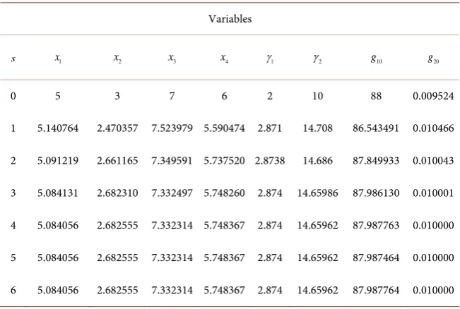
2 ,X 3 ,X 4 ,X 5 ,X 6 and the

corres-ponding objective function values g10 and g20 are given in Table 1. As seen

in Table 1, the absolute value of the difference between the points X(5) and X(5)

is reduced enough to a smaller value, and the iteration is terminated. One of the points X

( )

5 or X

( )

6 can be assumed the par to optimal solution point of the

given MOGPP for the weights w1=0.5, w2=0.5.

By considering different values of w1 and w2, the corresponding solutions

of the problem applying the taylor approach in each iteration are given in Table 2.

6. Result and Conclusion

In this study, we proposed an alternative approach to the approximate pare to solution of MOGPP based on the weighting method. In this model, MOGPP has been reduced to a sequential linear programming problem and the Pareto op-timal solution of MOGPP has been calculated approximately in an easier and more speedy way. Besides in GP problems and MOGPP the solution becomes more difficult when the degree of difficulty is a positive number whereas such a difficulty does not exist in the developed model. The solution for the problem given in the example by the weighted mean method is shown in Table 3 and the

Table 1. The corresponding iteration solution for w1=0.5 and w2=0.5, using the

Taylor series approach.

Variables

s x1 x2 x3 x4 γ1 γ2 g10 g20

0 5 3 7 6 2 10 88 0.009524

1 5.140764 2.470357 7.523979 5.590474 2.871 14.708 86.543491 0.010466

2 5.091219 2.661165 7.349591 5.737520 2.8738 14.686 87.849933 0.010043

3 5.084131 2.682310 7.332497 5.748260 2.874 14.65986 87.986130 0.010001

4 5.084056 2.682555 7.332314 5.748367 2.874 14.65962 87.987763 0.010000

5 5.084056 2.682555 7.332314 5.748367 2.874 14.65962 87.987464 0.010000

[image:12.595.213.539.513.732.2]

[image:13.595.211.539.90.285.2]

Table 2. The solution from the numerical approach method.

Variables

1

w w2 x1 x2 x3 x4 g10 g20 s

0.1 0.9 5.084056 2.682555 7.332314 5.748367 87.987764 0.01000 5 0.2 0.8 5.084056 2.682555 7.332314 5.748367 87.987764 0.01000 5 0.3 0.7 5.084056 2.682555 7.332314 5.748367 87.987762 0.01000 5 0.4 0.6 5.084056 2.682555 7.332314 5.748367 87.987764 0.01000 5 0.5 0.5 5.084056 2.682555 7.332314 5.748367 87.987764 0.01000 6 0.6 0.4 5.084056 2.682555 7.332314 5.748367 87.987764 0.01000 4 0.7 0.3 5.084056 2.682555 7.332314 5.748367 87.987764 0.01000 5 0.8 0.2 5.084056 2.682555 7.332314 5.748367 87.987764 0.01000 5 0.9 0.1 5.084056 2.682555 7.332314 5.748367 87.987764 0.01000 5

Table 3. Primal solutions [15].

Variables

1

w w2 x1 x2 x3 x4 Z

0.1 0.9 5.084055 2.682555 7.332315 5.748367 8.08776 0.2 0.8 5.084055 2.682555 7.332315 5.748367 8.08776 0.3 0.7 5.084055 2.682555 7.332315 5.748367 8.08776 0.4 0.6 5.084055 2.682555 7.332315 5.748367 8.08776 0.5 0.5 5.084055 2.682555 7.332315 5.748367 8.08776

solution by the model that we developed is shown in Table 2 and the results are almost the same. For this reason, proposed method can be used as an alternative of weighted mean method.

References

[1] Zener, C. (1961) A Mathematical Aid in Optimizing Engineering Design. Proceed-ings of National Academy of Sciences, 47, 537-539.

https://doi.org/10.1073/pnas.47.4.537

[2] Duffin, R.J., Peterson E.L. and Zener, C. (1967) Geometric Programming: Theory and Application. John Wiley and Sons, New York.

[3] Chiang, M. (2005) Geometric Programming for Communication Systems. Now Publishers Inc., Boston.

[4] Choi, J.C. and Bricker, D.L. (1996) Effectiveness of a Geometric Programming Al-gorithm for Optimization of Machining Economics Models. Computers & Opera-tions Research, 23, 957-961. https://doi.org/10.1016/0305-0548(96)00008-1

[5] Liu, S.T. (2007) Geometric Programming with Fuzzy Parameters in Engineering Optimization. International Journal of Approximate Reasoning, 46, 484-498.

https://doi.org/10.1016/j.ijar.2007.01.004

[image:13.595.208.540.320.442.2]

Conference, Baltimore, 30 June-2 July 2010, 3069-3074.

[7] Elmaghraby, S.E. and Morgan, C.D. (2007) Resource Allocation in Activity Net-works under Stochastic Conditions: A Geometric Programming-Sample Path Op-timization Approach. Tijdschrift voor Economie en Management, 52, 367-389. [8] Chu, C. and Wong, D.F. (2001) VLSI Circuit Performance Optimization by

Geo-metric Programming. Annals of Operations Research, 105, 37-60.

https://doi.org/10.1023/A:1013345330079

[9] Scott, C.H. and Jefferson, T.R. (1995) Allocation of Resources in Project Manage-ment. International Journal of System Science, 26, 413-420.

https://doi.org/10.1080/00207729508929042

[10] Jung, H. and Klein, C.M. (2001) Optimal Inventory Policies under Decreasing Cost Functions via Geometric Programming. European Journal of Operational Research, 132, 628-642. https://doi.org/10.1016/S0377-2217(00)00168-5

[11] Nasseri, S.H. and Alizadeh, Z. (2014) Optimized Solution of a Two-Bar Truss Non-linear Problem Using Fuzzy Geometric Programming. Journal Nonlinear Analysis and Application, 2014, 1-9. https://doi.org/10.5899/2014/jnaa-00230

[12] Islam, S. (2010) Multi-Objective Geometric Programming Problem and Its Applica-tions. Yugoslav Journal of Operations Research, 20, 213-227.

https://doi.org/10.2298/YJOR1002213I

[13] Biswal, M.P. (1992) Fuzzy Programming Technique to Solve Multi-Objective Geo-metric Programming Problems. Fuzzy Sets and Systems, 51, 67-71.

https://doi.org/10.1016/0165-0114(92)90076-G

[14] Verma, R.K. (1990) Fuzzy Geometric Programming with Several Objective Func-tions. Fuzzy Sets and Systems, 35, 115-120.

https://doi.org/10.1016/0165-0114(90)90024-Z

[15] Ojha, A.K. and Biswal, K.K. (2010) Multi-Objective Geometric Programming Prob-lem with Weighted Mean Method. International Journal of Computer Science and Information Security, 7, 82-86.

[16] Toksarı, M.D. (2008) Taylor Series Approach to Fuzzy Multiobjective Linear Frac-tional Programming. Information Sciences, 178, 1189-1204.

https://doi.org/10.1016/j.ins.2007.06.010

[17] Güzel, N. and Sivri, M. (2005) Taylor Series Solution of Multi Objective Linear Fractional Programming Problem. Trakya University Journal of Science, 6, 91-98. [18] Boyd, S., Kim, S.J., Vandenberghe, L. and Hassibi, A. (2007) A Tutorial on

Geome-tric Programming. Optimization and Engineering, 8, 67-127.

https://doi.org/10.1007/s11081-007-9001-7

[19] Geoffrion, A.M. (1968) Proper Efficiency and the Theory of Vector Maximization. Journal of Mathematical Analysis and Applications, 22, 618-630.

https://doi.org/10.1016/0022-247X(68)90201-1

[20] Caramia, M. and Dell’Olmo, P. (2008) Multi-Objective Management in Freight Lo-gistics. Springer, London.

[21] Bazaraa, S., Sherali, H.D. and Shetty, C.M. (2006) Nonlinear Programming Theory and Algorithms. 3rd Edition, John Wiley and Sons, New York.

https://doi.org/10.1002/0471787779

[22] Kwak, N.K. (1973) Mathematical Programming with Business Applications. McGraw- Hill, New York.

[24] Luptacik, M. (2010) Mathematical Optimization and Economic Analysis. Springer, New York. https://doi.org/10.1007/978-0-387-89552-9

[25] Ota, R.R. and Ojha, A.K. (2015) A Comparative Study on Optimization Techniques

for Solving Multi-Objective Geometric Programming Problems. Applied Mathe-matical Sciences, 9, 1077-1085.https://doi.org/10.12988/ams.2015.4121029

Submit or recommend next manuscript to SCIRP and we will provide best service for you:

Accepting pre-submission inquiries through Email, Facebook, LinkedIn, Twitter, etc. A wide selection of journals (inclusive of 9 subjects, more than 200 journals)

Providing 24-hour high-quality service User-friendly online submission system Fair and swift peer-review system

Efficient typesetting and proofreading procedure

Display of the result of downloads and visits, as well as the number of cited articles Maximum dissemination of your research work

Submit your manuscript at: http://papersubmission.scirp.org/