Buffer Occupancy of Double-Buffer Traffic Shaper in
Real-Time Multimedia Applications across Slow-Speed
Links
Ayodeji O. Oluwatope, Damilola T. Oyewo, Folake E. Olayiwola, Ganiyu A. Aderounmu, Emmanuel A. Adagunodo
Comnetlab, Network Utility Maximisation Sub-Group, Computer Science and Engineering, Obafemi Awolowo University, Ile-Ife, Nigeria
Email: [email protected]
Received October 17,2012; revised November 19, 2012; accepted December 21, 2012
ABSTRACT
In this paper, a double-buffer traffic shaper was investigated to adjust video frame rate inflow into the TCP sender-buffer of a multimedia application source across a slow-speed link. In order to guarantee QoS across a slow-speed link (i.e. < 1 MBPS), the double-buffer traffic shaper was developed. In this paper, the buffer size dynamics of double-buffer was investigated. The arrival and departure of frames were modeled as a stochastic process. The transition matrix for the process was generated and the stationary probability computed. A simulation program was written in Matlab 7.0 to monitor the buffer fullness of the second buffer when a 3600 seconds H.263 encoder trace data was used as test data. In the second buffer, it was discovered that over 90% of the play-time, the buffer occupancy was upper bounded at 300 frames per second and utilization maintained below 30%.
Keywords: Multimedia Application; Slow-Speed Link; TCP; Buffer Occupancy; QoS
1. Introduction
Over the years, there has been an unimaginable growth in the usage of the Internet across the globe. However, the range of applications being deployed across the Internet today is far broader than it was a few years back [1]. As it can be observed, traditional applications such as bulk file transfer (e.g. E-mail), and static websites are no longer sufficient for today’s Internet requirement, hence the need for the deployment of wider spectrum of applications. Applications that rely on the real-time delivery of data, such as video conferencing tools, Internet telephony, as well as video and audio streaming (referred to as multi- media applications) are fast gaining prominence in the Internet application space [1,2]. Video streaming, a mul- timedia application enables simultaneous delivery and playback of the video which overcomes the problems associated with file download since users do not have to wait for the entire video to be received before viewing it [3]. There are two types of streaming applications de-pending on whether the video is pre-encoded and stored for later viewing, or it is captured and encoded for real-time communication [4]. These new applications (real-time multimedia streaming, video-on-demand etc.) have diverse quality of service (QoS) requirements that are significantly different from traditional best effort ser-
across the network. It automatically regulates the video frames rates according to network congestion level [13]. Traffic shaper represents a complete system that provides high interactivity while adapting to a poor network con- dition [14]. This is achieved by adjusting transmission rate and controlling the quality of the received streams. Token bucket and Leaky bucket are techniques used to implement the double-buffer traffic shaper [15].
2. Relative Works
Real-time multimedia application transmission has been an active area of research. [16] studied an efficient delay distribution scheme that allocates the end-to-end delay bound into the end-station shaper and the network. They reviewed the effect of switch delay and shaping on net- work performance based on the empirical envelope traf- fic model, and analyzed the impact of shaping via com- puter simulations [1] offered a system design and im- plementation that ameliorates some of the important problems with video streaming over the Internet. He lev- eraged the characteristics of MPEG-4 to selectively re- transmit the most important data in order to limit the propagation of errors. [5] presented an implementation of an end-to-end application for streaming stored MPEG-4 Fine-Grained Scalable (FGS) videos over the best-effort Internet. There scheme adapts the coding rate of the streaming video to the variations of the available band- width for the connection, while smoothing changes in image quality between consecutive video scenes. Ioan and Niculescu in [17] proposed two mathematical models of an algorithm named Leaky bucket mechanism used for the parameter usage of connection control in multimedia networks.Bajic et al., in [18] addressed the issue of robust and efficient scalable video communication by integrat- ing an end-to-end buffer management and congestion control at the source with the frame rate playout adjust- ment mechanism at the receiver. Lam et al., in [19] ad- dressed the challenge of the lack of end-to-end quality of service support in the current Internet which caused sig- nificant difficulties to ensuring playback continuity in video streaming applications by investigating a new ad- aptation algorithm to adjust the bit-rate of video data in response to the network bandwidth available to improve playback continuity. In [20], Dubious and Chiustudied statistical multiplexing of VBR video in ATM networks. ATM promises to provide high speed real-time multi- point to central video transmission for telemedicine
ap-icantly improved streaming quality compared with the non-control policy. [13] asserted that the great end- to-end delays are the major factor influencing the vis-ual qvis-uality of real-time video across the Internet using TCP as transport layer protocol. Xiong et al. in [21] again pointed the requirement for transmitting real-time video with acceptable playing performance via TCP and presented a stochastic prediction model which can pre-dict the sending delays of video frames.
However, these available frame rate adaptation tech- niques are not suited for slow speed network environ- ment. It is therefore imperative to develop a new tech- nique that will meet this challenge. Double buffer traffic shaper is thus presented.
3. The Proposed Scheme (DBTS) Description
3.1. Video Transmission over the Internet
As described in our earlier paper, the first step in the transmission of video is compression of the raw video us- ing encoding coder-decoder scheme (CODEC) such as H.263, H.264, etc. at the sender-end [22,23]. The com- pressed video is passed to the sender-buffer within the application layer, thereafter passed to the TCP sender- buffer wherein they are fragmented into TCP data pack- ets. From within the TCP sender-buffer the fragmented video frames are moved into the network. The video frames are later received into a TCP receiver-buffer wherein they are defragmented and decompressed. The decompressed video frames are then sent into the re- ceiver playout-buffer. Figure 1 depicts the stage by stage
transmission of video frames from the sender to the re- ceiver across the internet.
3.2. The Double-Buffer Traffic Shaper (DBTS)
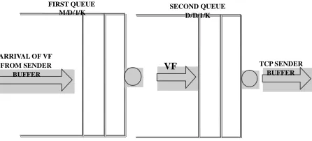
Because of the bursty nature of video frames traffics when released from the sender buffer [24], a network of two buffers in tandem is being introduced to model the Double-Buffer Traffic Shaper (DBTS) being proposed. A network of buffers is a collection of service centers which represent the server of the buffer and the custom-ers which represent video frames being transmitted [25]. As shown in Figure 2, the first queue models the
dy-namics of first queue as an “M/D/1/K” and the other, models the dynamics of the second queue as a “D/D/1/K” while the service discipline for the two buffers is FIFO (First-In-First Out). The two buffers are in an open queu-
Figure 1. Stages involved in the transmission of video frames from the sender to the receiver across the internet.
ARRIVAL OF VF FROM SENDER
BUFFER
FIRST QUEUE SECOND QUEUE M/D/1/K D/D/1/K
VF TCP SENDER BUFFER
Figure 2. Network of queues modeling of the proposed model.
ing network where jobs enter and depart from the net-work. “M/D/1/K” is interpreted as the arrival rate being markovian [26] and the departure rate is deterministic at the feeding the second buffer, thereby ensuring that frame out flow from the second buffer is maintained at a constant rate. Video frames thereafter are sent into sender’s TCP-buffer, hence achieving rate-adaptation. The frames flow dynamics can be expressed as a birth and death process. The transition is precipitated on H.263 encoder which sends an average of 10 frames per second [25,26]. The arrival rate into the queue is Poisson, which implies that frames arrive in bursts (irregular spurts). The service rate is deterministic with mean departure rate,
frames per second depending on the size of the queue. The inter-arrival rate in second queue of Figure 2
is inherited from the departure rate of the previous queue. There is a direct relationship between the two because the frame outflow of the M/D/1/K queue forms the in-flow into the D/D/1/K queue.
3.3. Stochastic Processes
Formally, a stochastic model is one represented as a sto-chastic process. A stosto-chastic process is a set of random variables
X t t T
,
X t
X t
where T is the index of set and taken to represent time.
The above stochastic process has the following prop-erties:
1) is a Markov process. This implies that has the Markov or memoryless property: given the value of X t
at some time t T , the future path
X s for s t does not depend on the knowledge of the past history X u
for u t , i.e. for1 n n1
t t t
,
1 1 1 1
1 1
Pr , ,
Pr
n n n n
n n n n
X t x X t x X t x
X t x X t x (1)
2) X t
S
is irreducible. This implies that all states in the state space, , can be reached from all other states by following the transitions of the process.
X t
1, , and 1 , , 1
is stationary: for any 3)
n n
t t T t t T n
1 n X t 1 X t n
X t X t
F F
.
Then the process’s joint distributions are unaffected by the change in the time axis and so,
(2)
4) X t
and
t s
is time homogenous: the behavior of the system does not depend on time when it is observed. In particular, the transition rates between states are inde-pendent of the time at which the transition occurs. Thus for all , it follows that
Pr Pr k j k jX t x X t x
X s x X s x
(3)
3.4. Transition Rate Diagrams of Double-Buffer Traffic Shaper
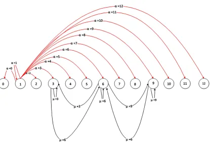
For Markov processes, the simplest way to represent the process is often in terms of its transition rate diagram. In this diagram, each state of the process is represented as a node in a graph. The arcs in the graph represent possible transitions between states of the processes. Since every transition is assumed to be governed by an exponential distribution, the rate of the transition becomes the pa-rameter of the distribution. In this paper, H.263 encoder transmits frame at an uneven rate. The range however is within 0 frames per second and 12 frames per second as shown in Figure 3. This also depicts the state space
[image:3.595.61.284.203.304.2]Figure 3. Transition rate diagram for M/D/1/K queue when α =1.
represents when the initial state is 1; it assumes that the first frame released by the encoder is 1.The service rate in Figure 3 is deterministic, so the queue serves a fixed
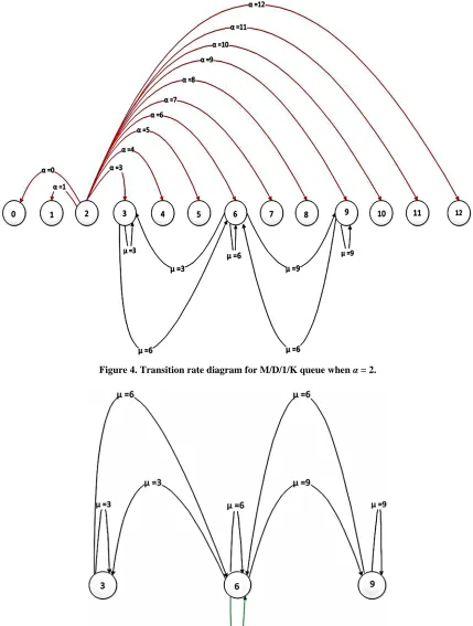
number of frames per unit time. However, the service rate in Figures 3 and 4 which model the first queue if α =
1, 2 in Figure 2 has to be regulated because it determines
the fullness of the second queue. Therefore, when the fullness of the second queue reaches a certain threshold, it informs the first queue to either decrease the frame rate to 3 frames per second or increase it to 9 frames per sec-ond. This informs the transition pattern that is observed in Figure 5. The initial state is state 6; but it can transit
to either state 3 or state 9 per second. The service rate of the first queue translates to the arrival rate of the second queue because they are connected together in series. Since the essence of DBFR is to obtain a constant bit rate, the server in the second queue serves only 6 frames per second which has been experimented to be suitable for a slow-speed of network that is <<< 1 Mbps. The parame-ters of distribution used in this paper are , , .
a t
They stand for the arrival rate of the first queue, service rate of the first queue and service rate of the second queue re-spectively.
3.5. Algorithm
Case 1: When current first queue size, , approaches
and above 75% capacity utilization, then current first queue outflow rate
be-longs to the set of positive real numbers.
If a t 0.75 then
1
y y
r t r t
1
y y
r t r t , where
Case 2: When current first queue size, a(t), operates
below 25% capacity utilization, then current first queue outflow rate is halved i.e. r ty 1
ry 0.0 1.0 , such that
Case 3: Otherwise, the flow rate is set at the default.
Assumptions:
Video frames inflow into First queue is Markovian utilizing the H.263 Standard. Second queue size is as-sumed larger than the First queue i.e.
ba
c c
. List of terms:
a —number of frames in first queue at time t , b—number of frames in second queue at time t, rx:
rate of Inflow to first queue, ry: rate of Inflow to second
queue, rz t
b
: rate of Inflow to the TCP sender buffer, : time(s) a: size of first queue (number of video frames), : size of Second queue (number of video frames).
Input: uneven arrival of video frames; Output: even departure of video frames,
Initialization: ca, cb, ry, rx,out: array [1,…,n].
rx← H.263 trace data.
begin:
ca(i+1) = ca(i) + rx(i);
if (ca(i) > 0.75 × a).
ry(i + 1)= ry(i) × ζ; else if (ca(i)< 0.25× a).
Figure 4. Transition rate diagram for M/D/1/K queue when α = 2.
cb(i +1) = cb(i) + ry(i + 1); if (cb(i + 1) > rz)
out(i) = rz;
cb(i + 1) = cb(i + 1) −rz; end.
end.
4. Derivation of Performance Measure—
Utilization
A Markov process with states can be characterized
by its . Matrix Q’s
entry in the column of the row of the matrix
n , tormatrix Q th i n finitesimalgenera th
nin j
j i q iis ij being the instantaneous transition rate. ij is the sum of the parameters labeling arcs connecting
states and
q
j in the transition rate diagram. The di-agonal elements are chosen to ensure that the sum of the elements in every row is zero, i.e.
,
j S j i ijq q
13
2, , 2, ,
, 2 and
d e e f
ii (4)
The infinitesimal generator matrix for the transition rate diagram of the M/D/1/K queue of Figure 3 is shown
in Equation (5). It is a 13 matrix, meaning that it has 13 states. The values for the parameters
1, , 2, , 2, , 2, , 2, , 2, , 2, , 2, , 2, a a a b b c c d
f g g h h i i j j k k l
, 2 4, 2 8, 2 12. d d h Q
Q 0
expressed in Equation (3.4) were obtained from the tran-sitions from one state to another. Therefore,
1 0, 2 1, 2 3, 2 3 2 5, 2 6, 2 7,
2 9, 2 10, 2 11,
a a a b b c c
e e f f g g h
i i j j k k l l
In solving the matrix Equation , in equation 5, the parameter values were inserted. The whole equation is thereafter transposed. i.e. 0 becomes QT
e
T n
4, 7 and 10
. This enabled the right hand side to be converted to col-umn vector of zeros rather than the initial row vector.
In other to resolve the problem of redundancy amongst the global balance equation, one of the global balance equations was replaced by the normalization condition. In the transposed matrix, this corresponds to replacing one row (last row) by a row of 1’s and also change the solution vector, which was all zeros to be a column vec-tor with 1 in the last row, and zero everywhere else. This vector is denoted by n, and the modified matrix is
de-noted by Q . It then becomes
or a subset of states which satisfy some condition. Therefore, utilization in the proposed model corresponds to those states in which service took place (states
x x
4 7 10
U
) on M/D/1/K Queue. i.e
x
0.0385 0.0769 0.1154 23.08%
U
The analytical utilization of M/D/1/K queue is about 23.08%.
5. Results and Discussion
Matlab 7.0 was used in simulating the proposed algorithm. H.263 trace data obtained from Verbose Jurassic stan- dard data set was used as the test data. The data file is a one-hour video session, and it is composed of 25,432 frames. Frame rate arrival into the first buffer was set
1, ,15
rx according to the principle of H.263 en-
coder. Arrival rate into the second buffer is obtained from the operation of the algorithm introduced at the server of the first queue.
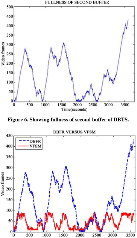
The volume of frames in the buffer is obtained from the accumulation of frames as a result of delay experi- enced by the frames. As shown in Figure 6, the initial
400 seconds of the video session shows a steady increase in the number of video frames to around 230 frames. The quantity however steadily reduced to zero within the proceeding 500 seconds. The volume rose to 250 frames at 1600 seconds and lingered at that point for 200 sec-onds. It thereafter dropped to less than 40 video frames for about 25% of the simulation period. It however peaked to 370 video frames towards the last 200 seconds of the simulation of the video session.
Again when the proposed scheme was compared with the existing scheme in terms of buffer occupancy, it was observed that the existing scheme outperformed the pro-posed scheme in most part of the simulation duration as can be seen in Figure 7. This performance is evident in
the overall quantity of frames in the buffer per unit time. Throughout the duration of the simulation, the quantity of frames in the existing scheme was constantly below 100 frames; it was highly bounded, while that of the proposed DBFR scheme hovered between 0 and 300 frames for more than 95% of the simulation duration.
For closer observation of the interesting points and disparities of the buffer fullness of the existing and pro- posed schemes, the simulation period was divided into six epochs.
Figure 6. Showing fullness of second buffer of DBTS.
[image:7.595.60.287.85.269.2] [image:7.595.60.285.295.488.2]Figure 7. Comparison of DBFR and VFSM schemes.
Figure 8 compares the two schemes for the first 200
seconds, it was noticed that for during the first 160 sec- onds, the proposed scheme performed excellently by maintaining a buffer fullness lower than the existing scheme. Figure 9 represents the buffer fullness between
200 - 700 seconds. This shows that the buffer fullness in the proposed scheme increased steadily to about 300 frames while the existing scheme did not exceed 100 frames. The two schemes later reduced the buffer full-ness during which the existing scheme crashed to as low as 3 to 10 frames for almost 50% of the time duration, the proposed scheme reduced buffer fullness to as low as 50 frames. In the third epoch shown in Figure 10, the
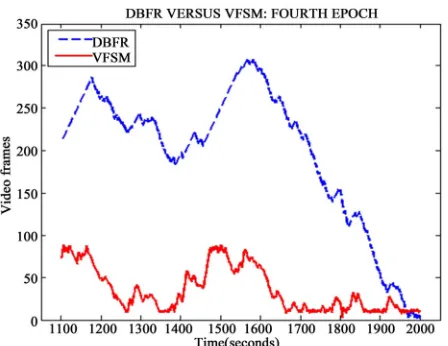
[image:7.595.310.535.304.482.2]two schemes’ performance was very close. They both maintained a fullness of about 50 frames throughout the duration (701 and 1100) seconds. Between 1101 and 2000 seconds, there was a remarkable difference in the performance of the two schemes as seen in Figure 11.
Figure 8. The first epoch of the comparison of DBFR and VFSM schemes.
Figure 9. The second epoch of the comparison of DBFR and VFSM schemes.
[image:7.595.313.532.524.703.2]Figure 11. The fourth epoch of the comparison of DBFR and VFSM schemes
[image:8.595.59.287.519.708.2]Figure 12. The fifth epoch of the comparison of DBFR and VFSM schemes
Figure 13. The sixth epoch of the comparison of DBFR and VFSM schemes.
schemes as noticed in Figure 12. The last epoch, shown
in Figure 13 lasted between 2781 and 3605. For the first
50%, the fullness in the proposed scheme was less than 160 frames. It however increased steadily to about 450 frames towards the end of the simulation, this experience lasted for less than 5% of the whole simulation duration.
Unfortunately, according to Little’s law, volume of frames in queue is equal to the product of arrival rate and means waiting time. This implies that the quantity of frames in the queue is directly proportional to the delay experienced by the frames in the queue. The delay that is experienced in the proposed scheme is expected to be greater than what is expected to be experienced in the existing scheme. Though the proposed scheme was able to achieve the purpose of its development, it is however being challenged with buffer fullness and packet delay being unbounded. The implication of this is that the in-frastructure provider would require more capital in pro-viding memory space. The user however only gets a bet-ter and improved video streaming quality.
6. Conclusion
In conclusion, it is evident that the proposed scheme was bounded to maximum of 300 frames per unit time for over 90% of the simulation time. This value is high when compared with the existing scheme (VFSM) which was bounded at less than 100 frames per unit time throughout the simulation time. However, the tripling value is justi-fiable because, it is opportunity cost for maintaining QoS along a slow-speed link for real-time multimedia appli-cation deployment across the Internet.
REFERENCES
[1] N. Feamster, “Adaptive Delivery of Real-Time Streaming Video,” Master’s Thesis, Department of Electrical Engi- neering and Computer Science, Massachusetts Institute of Technology,Cambridge, 2001.
[2] L. Tilley, “Computing Studies Multimedia Applications,” Number 1, Germany, 2005.
[3] G. Ji, “VBR Video Streaming over Wireless Networks,” Master’s Thesis, Department of Electrical and Computer Engineering, University of Toronto, Toronto, 2009, pp. 10-22.
[4] C. Huang, J. Li and K. W. Ross, “Can Internet Video- on-Demand Be Profitable?” ACM SIGCOMM Computer Communication Review, Vol. 37, No. 4, 2007, pp. 133- 144.
[5] M. Karakas, “Determination of Network Delay Distribu- tion of Network over the Internet,” Master’s Thesis, Mid- dle East Technical University, The Graduate School of Natural and Applied Sciences, Ankara, 2003.
[6] M. Salomoni and M. Bonfigle, “A Software Audio Ter- minal for Interactive Communications in Web-Based Educational Environments over the Internet,” In Booktitle, 1999.
http://www.cineca.it/nume03/Papers/IECON99/iecon2.htm [7] S.-J. Yang and H.-C. Chou, “Adaptive QoS Parameters
Approach to Modeling Internet Performance,” Interna- tional Journal of Network Management, Vol. 13, No. 1, 2003, pp. 69-82. doi:10.1002/nem.460
[8] C. Dinesh, H. Zhang and D. Ferrari, “Delay Jitter Control for Real-Time Communication in a Packet Switching Network,” IEEE Conference on Communications Soft- ware, “Communications for Distributed Applications and Systems”,18-19 April 1991, Chapel Hill, pp. 35-43. http://trace.kom.aau.dk/trace/tut/html
[9] D. Austerberry, “The Technology of Video and Audio Streaming,” 2nd Edition, Focal Press, Burlington, 2005. [10] J. Apostolopoulos, W. Tan and S. Wee, “Video Streaming:
Concepts, Algorithms and Systems,” Technical Report, Mobile and Media Systems Laboratory, HP Laboratories, Palo Alto, 2002.
[11] FCC, “Sixth Broadband Deployment Report,” Technical Report, Federal Communications Commission, 2010. http://www.fcc.gov/Daily-Releases/Daily-Busi-ness/2010 /db0720/FCC-10129A1.pdf
[12] P. de Cuetos, P. Guillote, K. Ross and D. Thoreau, “Im- plementation of Adaptive Streaming of Stored MPEG4 FGS Video over TCP,” IEEE International Conference on Multimedia and Expo, Vol. 1, 2002, pp. 405-408. doi:10.1109/ICME.2002.1035804
[13] Y. Xiong, M. Wu and W. Jia, “Efficient Frame Schedule Scheme for Real-Time Video Transmission across the Internet Using TCP,” Journal of Networks, Vol. 4, No. 3, 2009, pp. 216-223. doi:10.4304/jnw.4.3.216-223
[14] K. Ibrahim, “TCP Traffic Shaping in ATM Networks,” Department of Electronics, Faculty of Engineering and Architecture, Uludağ University, Bursa, 2000.
[15] B. A. Farouzan, “Data Communications and Network- ing,” 4th Edition, McGraw-Hill, New York, 2007. [16] Lee, B., Lim, H., Kang, H., and Kim, C. “A Study on
Efficient Delay Distribution Methods for Real-Time VBR Traffic Transfer,” Technical Report, Department of Com- puter Science, Seoul National University, Korea Institute of Advanced Engineering, Seoul, 1997.
[17] L. Ioan and G. Niculescu, “Two Mathematical Models fo Performance Evaluation of Leaky-Bucket Algorithm,” Revue Roumaine des Sciences Techniques Serie Electro- technique et Energetique, Vol. 50, No. 3, 2005, pp. 357- 372.
[18] O. Tickoo, A. Balan, S. Kalyanaraman and J. W. Woods, “Integrated End-to-End Buffer Management and Conges- tion Control for Scalable Video Communications,” In- ternational Conference on Image Processing, Barcelona, 14-17 September 2003, pp. 257-260.
[19] L. Lam, Y. Jack, B. Lee, S. Liew and W. Wang, “A Transparent Rate Adaptation Algorithm for Streaming Video over the Internet,” Department of Information En- gineering, The Chinese University of Hong Kong, Shatin, 2005.
[20] J. Dubious and H. Chiu, “High Speed Video Transmis- sion for Telemedicine Using ATM Technology,” Pro- ceedings of World Academy of Science, Engineering and Technology, Vol. 7, 2005, pp. 357-361.
[21] Y. Xiong, M. Wu and W. Jia, “Delay Prediction for Real-Time Video Adaptive Transmission over TCP,” Journal of multimedia, Vol. 5, No. 3, 2010, pp. 216-222. doi:10.4304/jmm.5.3.216-223
[22] J. Doggen and F. Van der Schueren, “Design and Simula- tion of a H.264 AVC Video Streaming Model,” Depart- ment of Applied Engineering, University College of Ant- werp, Antwerp, 2008.
[23] L. Arne and K. Jirka, “Evalvid-RA: Trace Driven Simula- tion of Rate Adaptive MPEG-4 VBR Video,” Department of Communication Systems, Technical University of Ber- lin, Berlin, 2007.
[24] Y. Won and B. Shim, “Empirical Study of VBR traffic Smoothing in Wireless Environment,” Division of Elec- trical and Computer Engineering Hanyang University, Seoul, 2002.
[25] X. Li, “Simulation: Queuing Models,” Technical Report, University of Tennessee, Knoxville, 2009.