Steady-State Behavior of Semiconductor Laser Diodes
Subject to Arbitrary Levels of External Optical Feedback
Qin Zou
Institut Mines-Telecom, Telecom SudParis, Département Electronique et Physique, UMR 5157 CNRS, Evry, France
and CEA Saclay Nano-Innov, Gif sur Yvette, France Email: [email protected]
Received November 21,2012; revised December 12, 2012; accepted December 30, 2012
ABSTRACT
This paper investigates the steady-state behavior of a semiconductor laser subject to arbitrary levels of external optical feedback by means of an iterative travelling-wave (ITW) model. Analytical expressions are developed based on an it-erative equation. We show that, as in good agreement with previous work, in the weak-feedback regime of operation except for a phase shift the ITW model will be simplified to the Lang-Kobayashi (LK) model, and that in the case where this phase shift is equal to zero the ITW model is identical to the LK model. The present work is of use in par-ticular for distinguishing the coherence-collapse regime from the strong-feedback regime where low-intensity-noise and narrow-linewidth laser operation would be possible at high feedback levels with re-stabilization of the compound laser system.
Keywords: Semiconductor Lasers; External Optical Feedback; Iterative Traveling-Wave Model; Compound Cavity Modes; Lang-Kobayashi Model; External Cavity Modes; Feedback Lasers
1. Introduction
Continuous efforts have been made since the last three decades on the dynamics of semiconductor lasers with external optical feedback, because of a large variety of interesting properties they exhibit. A laser with delayed feedback builds an ideal system for analyzing and ex- ploring typical phenomena encountered in a nonlinear time-delayed system, such as bifurcations, thresholds of instability (or stability) and routes to deterministic chaos. On the other hand, external optical feedback can severely affect the spectral behavior of a laser. It can also produce undesirable effects whose effective control is therefore essential for many applications such as optical-fiber- based transmission and sensor systems, since both of them are highly dependent on the spectral quality (tem- poral coherence and frequency stability) of the used light sources.
In parallel with numerous experimental investigations, theoretical approaches have also been developed aimed at a better understanding of the nonlinear dynamics of a compound laser system (see for example, Tromborg etal. [1], Schunk and Petermann [2], and Binder and Cormack [3]). Most of these approaches have been developed on the basis of the rate equations proposed by Lang and Kobayashi (LK) [4]. For the weak-feedback regime of operation (feedback power ratio less than −30 dB), these
approaches have been found to describe adequately vari-ous phenomena so far observed experimentally, such as the threshold of coherence collapse (CC), the low-fre- quency fluctuations (LFFs), and the period-doubling route to chaos [5]. The LK rate equations have also been used to explain the physical mechanisms of the steady-state [6] and transient [7] LFFs, as well as of the chaotic itiner-ancy for the case of relatively strong feedback [6].
It has been shown that the LK rate equations can be solved analytically by use of asymptotic methods (A de-tailed description can be found in [8]). In this approach, a laser with weak optical feedback is regarded as a weakly- perturbed nonlinear dynamic system and the threshold of instability corresponds to the first Hopf bifurcation of the LK rate equations. An attempt has been made at inter-preting experimental findings of InAs/InP quantum-dash Fabry-Perot lasers by using this approach, such as the onset of CC and the transition from the regime of LFFs to the regime of so-termed fully-developed coherence collapse (FDCC) [9].
justified. Thus, in order to describe the behavior of a feedback laser with arbitrary feedback levels, an iterative traveling-wave (ITW) model was developed [10,11]. By using this model, dynamic and noise properties of a laser subject to strong optical feedback were numerically in-vestigated [12]. The ITW model predicts in particular a significant decrease of the intensity noise in the strong- feedback regime.
More recently, Radziunas et al. used the traveling- wave (TW) approach proposed in [13,14] to model a feedback laser, where the system is described by partial differential equations for the electrical fields which counter-propagate along the longitudinal axis of the laser and are coupled through the usual carrier rate equation. A comparison has been made between the LK and TW models, with emphasis on the stability analysis of cavity modes in their continuous-wave states [15].
This paper investigates the steady-state behavior of a feedback laser with arbitrary feedback levels by means of the ITW model. It may be considered as an extension of the works of Langley etal. [12] and Spencer etal. [16]. We provide additional information about the physical insight into a compound laser system and discuss the similarities and the differences between the ITW and LK models. In Section 2, steady-state solutions will be de- rived for the external cavity modes and compared with previous work. In Sections 3 and 4, a detailed quantita- tive comparison between the ITW and LK models will be made and the rigorous condition will be given, under which the ITW model will be simplified to the LK model. Finally, Section 5 will summarize our conclusions.
2. Iterative Traveling-Wave Model
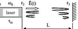
Consider the configuration of Figure 1. A single-longi- tudinal-mode laser diode is in resonance with an external Fabry-Perot cavity. We assume that r1, r2 and r3 are all
real and dispersionless. For this three-mirror system, the dominant resonator is defined by the mirrors with reflec- tion coefficients r1 and r3, and multiple round trips inside
the external cavity should be in general taken into ac- count for an arbitrary feedback level.
laser
L
τin
r2
ω0 Ẽ(t) r3 r1
laser
L
τin
r2
[image:2.595.111.242.596.645.2]ω0 Ẽ(t) r3 r1
Figure 1. Schematic drawing of a laser diode with external optical feedback. ω0: emission (angular) frequency of the
laser without feedback; τin: internal round-trip time; r1:
reflection coefficient of the rear facet of the laser; r2:
reflec-tion coefficient of the front facet of the laser; r3: reflection
coefficient of the external mirror; Ẽ(t): right-moving elec-tric field passing through the laser front facet; L: length of external cavity assumed empty.
2.1. Steady-State Solutions
The right-moving electrical field E t
, calculated at steps of the internal round-trip time τin (in seconds) satis- fies the following iterative equation [12,16]
2 2 22 2 3
0
1 exp 1
2 1 e in in N th M k k E t G
j N t N
r
E t r r r E t k jk
0 xp
(1) In this equation, GN (in s−1·m3) is the differential gain; α is the linewidth enhancement factor (LEF); N t
(in m−3) is the carrier density andth its threshold; τ (in seconds) is the external round-trip time and 0
N
(in rad,
0 0
) is the initial feedback phase associated with the emission frequency of the solitary laser operating near threshold.
By inserting E t
E t0
exp
j t
into Equation (1)and considering steady-state solutions, we obtain the following expressions for the excess gain (in s−1)
and the feedback phase Δ (in rad,
G
with ω: pos-sible emission frequency) due to the compound structure
2 24 2 1 1ln in D E G r
(2)
and 2 tg 0. 1 in E b D
(3) In the above two equations, D (dimensionless), E (di-mensionless) and b2 (in rad) are written respectively as
2
2 2 3
0
1 M kco
k
D r r r k
s
n
(4)
2
2 2 3
0
1 M ksi
k
E r r r k
(5)and
2 22 4
2 1 ln
2 2
in D E
b G
r
(6)
where 0 .
The steady-state behavior of a possible mode (with phase Δ and excess gain G) produced by a feedback laser under multiple-reflection configuration is described by Equations (2)-(6). We will show in Section 3 that in the case of low feedback levels , except for a phase shift, these equations will reduce to the well-em- ployed forms obtained from the LK rate equations. In the following, a cavity mode referred to the LK model will
r31
mode is referred to the ITW model, it will be called a compound cavity mode (CCM), as suggested in [15].
2.2. Initial Feedback Phase
edback phase
Let us first examine the initial fe 0. With
a given system, the phase (or normalized emi n fre- quency) Δ of a possible mode, being in dependence on
0
, is determined through the so-called phase equation. er the consideration of low feedback levels, the phase equation has a simpler form and two particular situations have been introduced and widely studied, where Δ is predefined and 0 is then determined from Δ. The first
situation corresp s to the “maximum gain mode” de-fined by the condition 0 mod 2
π
. This gives rise to
0 mod 2π
, w the feedback rate
[1,2]
ssio
Und
defi
ond
l by
here γ (in s−1) is
ned as usua
2
2 3
2
1 . in
r r r
(7)
In the second situation, the initial frequency remains unchanged
0
and the related mode is called the“minimum l mode”. We have thus
10 tg
inewidth .
We introduce here another category of modes, where
0 is determined directly from Equation (3). So by put-
r3 = 0 and M = 0 in Equations (4) and (5), we obtain 2
ting
tion (3 2 1
D r , E = 0 and, from Equation (6), b2 = 0. Equa-
comes then ) be
0 π 0, 1, 2, .
in
m m
(8)
It follows that the change of values is parameter-
iz 0
ed by the ratio in . We note that for both the “maximum gain mo and the “minimum linewidth mode” there exists the solution 0 0 (when 0
de”
), and that this corresponds to the z er solutio = 0) of Equation (8). For simplicity and principle demon- stration, we will use in the following 0 0 as the
value of the initial feedback phase. We wi that in the weak-feedback regime
r3 1
quantitative agree- ment between the ITW and dels can be obtained only with this initial phase value.ero
LK mo
-ord n (m
w ll sho
2.3. Excess Gain
gain written as
(9) where τp (in seconds) is the photon lifetim
A possible CCM has its
1
G G
p
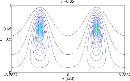
e and G is the excess gain due to feedback whose expres is given by Equation (2). A contour plot of the evolution of
G
as functions of Δ and r3 is shown in Figure 2. As
be seen from this figure, G peaks at the critical sion
[image:3.595.311.535.86.226.2]can
Figure 2. Contour plot of the excess gain ΔG in the vicinity
point r3 = r2, which correspo ds to a symmetrical (Fabry-
2.4. Modal Density of Photons
the carrier density N
of the initial feedback phase Δ0 (Δ0 = 0), as functions of the
CCM feedback phase Δ and the reflection coefficient r3, for
r2 = 0.65, α = 5, τin = 9 ps, τ = 0.9 ns, and M = 100.
n Perot) external cavity.
From the standard rate equation for
[1,4] and by assuming a linear relation between the gain G and N, we can derive the expression for the density of photons (or photon number) I (in m−3) of a CCM. Here I is calculated directly from E t
, we have thus in steady state2 0
1 p s
s N
p
G I
G I E
G
(10)
where Is is the density of photons for the solitary laser. It is written as
th
s p
s
N
I J
(11) where J (in s−1·m−3) is the pumping current and τs (in sec-
typical phenomenon can be observed from this fig- ur
onds) is the carrier life time. An example of the typical evolution of I as functions of Δ and r3 is shown in Figure
3. A
e: high values of the reflection coefficient r3 do have an
effect on enhancement of the density of photons. In this example, I is much higher in the strong-feedback regime than in the moderate-feedback regime (~5 × 10²⁰ m−3
against ~3 × 10²⁰ m−3, which is the threshold value I
Figure 3. Plot of the density of photons I in the vicinity of
ure 2(a), in [12]). We see from this figure that with in-
nomenon is related to the FDCC regime [7
the initial feedback phase Δ0 (Δ0 = 0) as functions of the
CCM feedback phase Δ ranging from −2π to 2π and the reflection coefficient r3, for r2 = 0.65. The values of the other
parameters are α = 5, τin = 9 ps, τ = 0.9 ns, τs = 2 ns, τp = 2 ps,
GN = 1.1 × 10⁻¹² s−1·m3, Is = 3 × 10²⁰ m−3, and M = 100.
creasing of r3, there are three well distinguished regimes
for the RIN: the weak-feedback regime (r3 < 0.005), the
noisy CC regime, and the strong-feedback regime (r3 >
0.1). The RIN increases in the CC regime as expected but decreases significantly (more than 10 dB/Hz) in the strong-feedback regime compared to its values in the weak-feedback regime. This result implies that a stable laser operation with low intensity-noise levels would be possible under the condition of strong feedback. In fact, stable and narrow-linewidth operation has been already observed with systems in configuration of strong optical feedback [17].
Another phe
]. This regime has been identified for a large pumping current, corresponding therefore to higher output power. In a recent investigation, InAs/InP quantum-dash Fabry- Perot lasers emitting at 1.57 μm were assessed for their tolerance to external optical feedback by using a free- space setup with a “short” (L = 0.5 m) external cavity [18]. In these experiments, the regime of FDCC was at-tained for a pumping current of about 30 mA at a rather high feedback level (−1.2 dB in terms of power ratio) with a 600-μm-long laser. As can be seen from the measured RF (radio frequency) spectra reported in this reference ([18], Figure 5(b)), the FDCC regime is char- acterized by a significant increase of the RF peak power around the relaxation oscillation frequency of the solitary laser, and hence by a high output power in steady state at high levels of feedback. We note that such a behavior manifested by a coherence-collapsed laser can be quite well understood using the formalism developed from the ITW model as can be seen from the RIN spectra simula- tions ([12], Figure 2(b)), and that the FDCC regime cor responds roughly to the beginning of the strong-feedback regime, as can be seen from the plot of photon density,
(a)
(b)
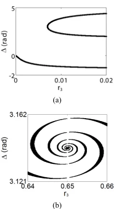
Figure 4. Zoom on two par lar regions in Figure 5. (a)
i.e. Figure 3, in the present text.
2.5. Phase Condition
vity structure, the phase
condi-s of the CCMcondi-s icondi-s sh
ticu
Region corresponding to small values of r3 (moderate-
feedback regime, where the use of the LK model may still be justified); (b) Whirl-shape region near the critical point r3 = r2, at which the maximum number of CCMs is found.
For a given compound-ca
tion determines the emission frequency of a possible CCM. The phase Δ associated with this mode should satisfy the transcendental Equation (3). In general only numerical solutions are possible.
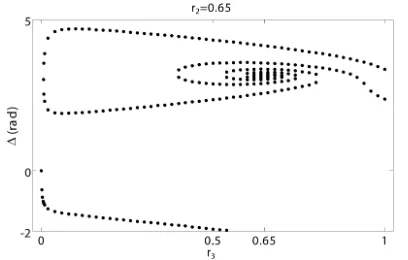
An example of bifurcation diagram
own in Figure 5. The value of each point was obtained by a numerical solution of Equation (3). For greater values, it will suffice to repeat the “pattern”. We pres t in Figure4 two particular regions in Figure5, where is found in (a) the shape predicted by the LK model as ex- pected. We see from Figure5 that, when r3 < r2, same as
a classical bifurcation pattern, all the modes (except the first mode 0
en
) emerge by pairs and their number pro- gressively increases with r3. The maximum number of
modes is attained at the point r3 = r2, corresponding to a
symmetrical external cavity. For r3 > r2, the modes will
disappear also by pairs. Finally, the number of modes will become minimal in the strong-feedback regime. We think that Figure 5 is equivalent to the bifurcation dia- gram for the normalized carrier density illustrated in [12] (Figure 4), showing clearly that high feedback levels can prevent a feedback laser from noisy output.
3. Convergence to the Model of Lang and
In e will show that in the weak-feedback
Kobayashi
[image:4.595.58.290.84.223.2]Figure 5. Bifurcation diagram of the CCMs. The values of
regime , except for a phase term, the ITW
levels, there will be on
(12)
. (13) Inserting the above two equations into
an
the parameters are α = 5, τin = 9 ps, τ = 0.9 ns, Δ0 = 0, r2 =
0.65, and M = 100.
r3 1
ill reduce
model w to the LK model. Thus, in the case of low feedback
ly one reflection (M = 1). Equations (4) and (5) are simplified as
2
2 2 3
1 1 cos
D r r r
2
2 2 3
1 sin
E r r r
Equation (2) d using the approximations
2
2 3 2
1r r r 1 and
ln 1x x for small x values, w pres- eady-state excess gain
2 cos
G
e obtain the ex
(14) In the same way, for the phase Equatio
sion for the st
. n (3), we have
2
r r r
2 2 3
2 2 2
2 2 2 3
1 sin
tg
1 cos
in
b
r r r r
(15)
where
(16)
By making some approximations and using
2 in cos .
b
tg x x, we obtain the phase condition
cos sin
(17)
It follows that except for a phase shift , Equations (1
4. Diagram of the Photon Density versus the
It a laser operating in the weak-even
feedback level, the
0
e de
4) and (17) have the same forms as thos rived from the LK rate equations. This result confirms the work of Radziunas et al. [15]. They showed a good qualitative agreement between the ECM and CCM solutions at moderate feedback levels. They also found a quantitative agreement for low feedback levels.
Mode Phase
is known that formoderate-feedback regime a common way to represent the possible steady states of the ECMs at a fixed feed- back level is through an ellipse showing the density of photons I versus the feedback phase Δ, and that only a finite number of ECM points are possible which are all located on the ellipse [8,19].
For the case of an arbitrary I stab-diagram with a given pumping current J can be e lished first by expressing Δ as a function of G and then by combining the result with Equation ( . We have respectively from Equations (2) and (3)
10)
1
tg
2 in D 1
(18) and from Equations (14) and (17) for the case of
G E
3 1
r
2 2
4 .
2 2
G
G
(19)
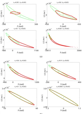
Figure 6 shows the plots of the I ly E
diagram for various values of r3, using respective quations (18)
and (19). Two typical phenomena inside the CC regime are clearly shown in this figure: a “banana”-like shape and a shift, to positive phase values, of the CCM fixed points due to the inclusion of multiple reflections in the ITW model, as also observed by Spencer etal. when they used the ITW model to establish the possible steady states in the I versus
2π
plane ([16], Figure 1). We also observe, in F a perfect overlap of the two ellipses for r3 = 0.003. This is because we have taken(for simplicity and principle demonstration) 0 0
igure 6,
as the initial phase value.
Finally, let us make a direct comparison between the iteration equation for the ITW model and the rate equa- tion for the LK model. It can easily be shown that at low feedback levels, any stationary solution to Equation (1) will lead to the following equation
1
exp
2 N
s th G
0
j N N j j
(20)
where Ns nd
is the steady-state carrier density. Under the same co ition, the LK rate equation will reduce to
01 2
exp 0.
N
s th
G
j N N
j j j
(21)
These two equations show, together with Equations (14) and (17), that the two models are strictly identical if and only if 0 0 [see also Figure 6(b) for r3 =
0.003].
5. Conclusions
itional information about the This paper provides add
(a)
[image:6.595.154.441.82.478.2](b)
Figure 6. Evolution of the I−Δ diagram as a function of r3 e diagrams are determined respectively from Equation (18)
developed based on an iterative travelling-wave model,
ber of modes is obtained w
ing that beyond the coherence-collapse regime, the sys-
for stable and no
. Th
(red curves, M = 100) and Equation (19) (green curves). The green dots refer to the solitary-laser solution. (a) r3 = 0.95, 0.8,
0.7 and 0.65; (b) r3 = 0.6, 0.4, 0.1 and 0.003. The values of the other parameters are r2 = 0.65, Δ0 = 0, α = 5, τin = 9 ps, τ = 0.9 ns,
τs = 2 ns, τp = 2 ps, GN = 1.1 × 10⁻¹² s−1·m3, and Is = 3 × 10²⁰ m−3.
which enable a characterization in a rigorous way of a cavity mode in its steady state. We show that with de- creasing of the reflection coefficient of the external mir- ror three regimes emerge successively which can clearly be distinguished from bifurcation diagram and gain plot: they are strong-feedback, coherence-collapse, and mod- erate-feedback regimes. This latter covers the weak- feedback regime where the use of the model of Lang and Kobayashi is entirely justified.
We find that maximum num
hen the external cavity becomes symmetrical. This state may cause a noisiest laser output. In the strong-feedback regime, a feedback laser is characterized by a minimum mode number and a high density of photons. This behav- ior confirms previous experimental observations, indicat-
tem could be re-stabilized and that as a result stable laser operation with low intensity-noise level could be ex- pected with external-mirror reflectivity close to 1. A novel class of modes has been proposed, which is pa- rameterized by the ratio between the external and internal round-trip times. We have also examined the similarities and the differences between the iterative travelling-wave and Lang-Kobayashi models. We find that in the weak- feedback regime these two models are identical only if the initial feedback phase is equal to zero.
The present work is above all useful for determination of the external feedback levels required
Future investigations will include a detailed analysis of the coherence-collapse regime by means of these two m
REFERENCES
[1] B. Tromborg, . Olesen, “Stability
Analysis for a an External
Cav-odels.
J. H. Osmundsen and H Semiconductor Laser in
ity,” IEEEJournalofQuantumElectronics, Vol. 20, No. 9, 1984, pp. 1023-1032. doi:10.1109/JQE.1984.1072508 [2] N. Schunk and K. Petermann, “Numerical Analysis of the
Feedback Regimes for a Single-Mode Semiconductor Laser with External Feedback,” IEEE Journalof Quan-tumElectronics, Vol. 24, No. 7, 1988, pp. 1242-1247. doi:10.1109/3.960
[3] J. O. Binder and G. D. Cormack, “Mode Selection an Stability of a Sem
d iconductor Laser with Weak Optical Feedback,” IEEE Journal of QuantumElectronics, Vol. 25, No. 11, 1989, pp. 2255-2259. doi:10.1109/3.42053 [4] R. Lang and K. Kobayashi, “External Optical Feedback
Effects on Semiconductor Injection Laser Properties,” IEEE Journal of Quantum Electronics, Vol. 16, No. 3, 1980, pp. 347-355. doi:10.1109/JQE.1980.1070479 [5] J. Ye, H. Li, and J. G. McInerney, “Period-Doubling
Route to Chaos in a Semiconductor Laser with Weak Op-tical Feedback,” PhysicalReviewA, Vol. 47, No. 3, 1993, pp. 2249-2252. doi:10.1103/PhysRevA.47.2249
[6] T. Sano, “Antimode Dynamics and Chaotic Itinerancy in the Coherence Collapse of Semiconductor Lasers with Optical Feedback,” PhysicalReview A, Vol. 50, No. 3, 1994, pp. 2719-2726. doi:10.1103/PhysRevA.50.2719 [7] J. Zamora-Munt, C. Masoller and J. García-Ojalvo,
“Transient Low-Frequency Fluctuations in Semiconduc-tor Lasers with Optical Feedback,” Physical Review A, Vol. 81, No. 3, 2010, Article ID: 033820.
doi:10.1103/PhysRevA.81.033820 [8] T. Erneux and P. Glorieux, “Laser Dyn
bridge University Press, New York,
amics,” 2010.
der Extern
ave Line Model for Laser
. Shore and J. Mørk, “Dynamical and
[9] Q. Zou and S. Azouigui, “Analysis of Coherence-Col- lapse Regime of Semiconductor Lasers un al Optical Feedback by Perturbation Method,” Chapter 5, Semiconductor Laser Diode Technology and Applications, Edition InTech, 2012, pp. 71-86.
[10] J. Mørk, “Rep. S48,” Danish Center for Applied
Mathe-matics and Mechanics, 1989. [11] F. Sporleder, “Travelling W
Diodes with External Optical Feedback,” Proceedingsof the URSI International Symposium on Electromagnetic Theory, International Union of Radio Science, Brussels, 1983, pp. 585-588.
[12] L. N. Langley, K. A
Noise Properties of Laser Diodes Subject to Strong Opti-cal Feedback,” OpticsLetters, Vol. 19, No. 24, 1994, pp. 2137-2139. doi:10.1364/OL.19.002137
[13] J. E. Carroll, J. Whiteaway and R. Plumb, “Distributed
delow, M. Radziunas, J. Sieber and M. Wolfrum, Feedback Semiconductor Lasers,” InstitutionofElectrical Engineers, London and SPIE Optical Engineering Press, 1998.
[14] U. Ban
“Impact of Gain Dispersion on the Spatio-Temporal Dy-namics of Multisection Lasers,” IEEE Journalof Quan-tumElectronics, Vol. 37, No. 2, 2001, pp. 183-188. doi:10.1109/3.903067
[15] M. Radziunas, H. J. Wünsche, B. Krauskopf and M. Wolfrum, “External Cavity Modes in Lang-Kobayashi and Traveling Wave Models,” Proceedings ofSPIE,Vol. 6184, 2006. doi:10.1117/12.663546
[16] P. S. Spencer, C. R. Mirasso and K. A. Shore, “Effect of Strong Optical Feedback on Vertical-Cavity Surface- Emitting Lasers,” IEEE Photonics Technology Letters, Vol. 10, No. 2, 1998, pp. 191-193.
doi:10.1109/68.655354
[17] C. E. Weiman and L. Holberg, “Using Diode Lasers for
Kelleher, S. P. Hegarty, G. Huyet, B. Atomic Physics,” Review of Scientific Instruments, Vol. 62, No. 1, 1991.
[18] S. Azouigui, B.
Dagens, F. Lelarge, A. Accard, D. Make, O. Le Gou-ezigou, K. Merghem, A. Martinez, Q. Zou and A. Ram-dane, “Coherence Collapse and Low-Frequency Fluctua-tions in Quantum-Dash Based Lasers Emitting at 1.57 μm,” OpticsExpress, Vol. 15, No. 21, 2007, pp. 14155- 14162. doi:10.1364/OE.15.014155
[19] C. H. Henry and R. F. Kazarinov, “Instability of Semi-conductor Lasers Due to Optical Feedback from Distant Reflectors,” IEEEJournalofQuantum Electronics, Vol. 22, No. 2, 1986, pp. 294-301.