Munich Personal RePEc Archive
Research and Development of an
Optimally Regulated Monopolist with
Unknown Costs
SAGLAM, ISMAIL
Ipek University
27 November 2014
Research and Development of an Optimally
Regulated Monopolist with Unknown Costs
Ismail Saglam
∗Department of Economics, Ipek University Turan Gunes Bulvari 648. Cad., Oran
Cankaya, Ankara 06550, Turkey
Abstract
This paper studies whether a monopolist with private marginal cost information has incen-tives to make cost-reducing innovations through research and development (R&D) when its output and price are regulated according to the incentive-compatible mechanism of Baron and Myerson (1982). Under several assumptions concerning the cost of R&D and the regu-lator’s beliefs about the marginal cost, we characterize the optimal level of R&D activities for the regulated monopolist when these activities are observed by the regulator as well as when they are not. We show that the regulated monopolist always chooses a higher level of R&D activities when its activities are unobserved. In situations where the social welfare attaches a sufficiently high weight to the monopolist welfare, the monopolist’s R&D activities in the unobservable case even realize at a higher level than its activities when its output and price are not regulated. Moreover, whenever R&D activities increase pro-ductive efficiency, a less efficient monopolist would choose a higher level of R&D activities than a more efficient monopolist, irrespective of the observability of R&D.
Keywords: Monopoly; Regulation; Research and Development.
JEL Classification Numbers: D82, L51, O32
1
Introduction
Regulating a natural monopolist with unknown costs has been extensively studied in the economic literature since the early work of Dupuit (1844, 1952). However, the first systematic approach is due to Baron and Myerson (B-M) (1982), who introduced a general social welfare as a function of possible costs and characterized an optimal set of regulatory rules maximizing the expected value of this welfare. Formally, B-M restricted themselves by the Revelation Principle [see Dasgupta, Hammond and Maskin (1979), Myerson (1979), and Harris and Townsend (1981)] to incentive-compatible mechanisms that require the monopolist to report its unknown marginal cost and ensure that it has no incentive to lie. The regulatory mechanism proposed by B-M involves four policy schedules: a price schedule and a quantity schedule which must be consistent with each other on the market demand curve, a subsidy schedule specifying at each marginal cost level the monetary transfer from consumers to the monopolist, and also a probability schedule specifying the range of marginal costs at which the monopolist will be allowed to sell. Given any mechanism that respects the incentive-compatibility condition, the regulator can calculate at each marginal cost level the required net profits the monopolist must obtain, and resultingly the subsidy it must receive, to truthfully reveal its unknown cost parameter. Consumer surplus net of this incentive-compatible subsidy constitutes consumer welfare. On the other hand, for any given α in [0,1], consumer welfare plus α fraction of the monopolist’s net profits (producer welfare) is called the social welfare. Since the monopolist’s marginal cost parameter will be known to the regulator only after she has announced the regulatory mechanism, any welfare consideration the regulator may have before the revelation of the cost parameter can only be of a Bayesian nature. Thus, it is necessary to define the expected social welfare, calculating the mathematical expectation of the social welfare under the regulator’s prior beliefs about the unknown marginal cost over a given support. The problem of the regulator is then to choose among all feasible policy schedules, the optimal schedules under which the expected social welfare will attain its maximum. Given the value of α
at θ. Resultingly, the optimal output schedule lies below the given market demand curve almost everywhere. On the other hand, the optimal probability schedule allows the monopolist to sell at any marginal cost level provided that the induced consumer surplus at the optimal output and price exceeds the fixed cost of production. Finally, the optimal subsidy schedule requires that the monopolist truthfully reporting its marginal cost as θ receives a subsidy so high that its welfare equals the area under the optimal output schedule within the range of possible marginal costs not lower than θ but also not higher than a critical level above which the optimal probability schedule prohibits the monopolist from selling its product.
In this paper, we would like to study the question “whether the optimal regu-latory mechanism of B-M, which provides large enough incentives to the regulated monopolist for truthfully revealing its private marginal cost, also has any incentives for the same monopolist to make cost-reducing research and development (R&D) in a static framework?” To answer this question, we will extend the model of B-M by adding a pre-regulatory stage in which the monopolist has access to an R&D tech-nology determined by a publicly known parameter γ ∈(0,1) and a control variable
ρ ∈ [0,1). Basically, this technology will reduce the private marginal cost of the monopolist from θ to γθ with probability ρ. The parameter γ will be called the improvement of (successful) R&D. On the other hand, the variable ρ will be deter-mined by the level of R&D activities, and will be called the probability of success or the level of R&D activities interchangeably. We will close our model by defining an R&D cost function with some convenient properties.
Clearly, our assumption that the regulator is completely informed about the im-provement level of R&D, or relatedly the parameter γ, will simplify our research problem quite a lot. In situations this assumption does not hold, the regulated firm would
problem. [Baron and Besanko (1984, p. 268).]
Likewise, we will either completely get rid of (as in Section 3.1) or enormously simplify (as in Section 3.2) a similar moral hazard problem that might otherwise have arisen - in a nontrivial way - with regard to the regulator’s information about the success likelihoodρ, by assuming that the variable ρ, which is directly controlled by the monopolist’s R&D activities, is either completely observable or completely un-observable to the regulator. However, despite the simplicity of the R&D technology stemming from these (analytically) extreme informational assumptions, the question we have asked above, regarding the desirability of R&D for a monopolist regulated under (any nondegenerate form of) the B-M mechanism, cannot be straightforwardly answered like in the case where the production of the same monopolist is not regu-lated. Obviously, for the unregulated monopolist, any decrease in the marginal cost would directly increase its expected marginal profit at all output levels since its ex-pected marginal revenues are independent of R&D. Thus, when the cost of R&D is sufficiently small, the additional profit the monopolist can expect to earn under R&D is always positive even if the monopolist chooses not to change the quantity of its output accordingly. The monopolist could exploit this opportunity by choosing the level of R&D activities at a point that would simply balance the constant marginal benefits and varying marginal costs of R&D.
model coincides with the market demand function whenα = 1, so the output at the truthfully reported marginal cost of the monopolist implies marginal cost pricing, as well. Therefore, in both models the monopolist’s gross surplus calculated at the realised output level, i.e., the marginal benefit of R&D, becomes independent of the level of R&D activities. Consequently, when α = 1, to calculate the optimal R&D in the case the monopolist is regulated by the B-M mechanism is as straightforward as to calculate it in the case the monopolist is unregulated.
It is also clear that regardless what the value of the welfare parameter α is, the monopolist would like to have been endowed, before it was introduced to the given regulatory environment, with a lower marginal cost to exploit higher informational rents, since the marginal informational rent is always positive. However, whether the monopolist can benefit from reducing its present cost of production through R&D is not clear when α 6= 1, even in situations where the cost of R&D is negligible. The reason is that the awareness of a Bayesian regulator about the R&D activities of the monopolist could lead her to revise her beliefs in such a way that the adjusted demand would be lower at each price level.1 Thus, although a likely cost reduction
through R&D could increase the range of potential costs over which marginal infor-mational rent will be collected, the downward shift of the adjusted demand curve would suppress the marginal informational rent at each cost level, hence the ambigu-ity. With some assumptions on the regulator’s beliefs and R&D costs, we will get rid of this ambiguity in Section 3.1, where we will characterize the optimal level of R&D activities chosen by the monopolist when its choice is observable by the regulator (before she announces her beliefs to the public). We will study in Section 3.2 the polar case where the R&D activities of the monopolist are never observable. In fact, this case may be more realistic than the previous case, since
1
‘Although the regulator may be able to observe dollar outlays allo-cated to R&D projects that are ostensibly aimed at cost reduction, he cannot monitor precisely the manner in which these funds are actually employed, nor can he certify the level of intensity or dedication with which the R&D efforts are actually pursued.’ [Sappington (1982, p.355).]
In both Section 3.1 and Section 3.2, we will also study how the optimal R&D choice of the monopolist is affected by several parameters of our model, including the efficiency of the monopolist, the improvement level of the R&D technology, the weight of the monopolist welfare relative to consumer welfare, and the maximal size of demand. In Section 3.3 we will compare the characterization results in Sections 3.1 and 3.2 to establish that the monopolist always chooses a higher level of R&D activities when its activities are unobservable than when they are observable. Fur-thermore, in Section 3.4 we will show that in situations where the social welfare attaches a sufficiently high weight to the monopolist welfare, the unobservable R&D activities of a regulated monopolist will even realize at a higher level than the activ-ities of an unregulated monopolist. Finally, we will conclude in Section 4.
We should note here that a problem similar to ours was earlier studied, mostly in dynamic setups, by a handful of papers. For example, for a two-period monopoly, Baron and Besanko (1984) considered regulation and innovation through R&D.2
Lewis and Yildirim (2002) studied, in an infinite horizon model with asymmetric cost information, the optimal regulation of an innovating monopoly that learns from past experiences. Giuseppe and Vincenti (2004) explored in a multi-period model the effect of price-cap regulation on cost-reducing efforts. The closest paper to ours is that of Sappington (1982), who also studied the R&D problem of a single-period monopoly. However, his informational assumptions as well as his research question
2
are different from ours.3 To the best of our knowledge, the existing regulation
lit-erature is lacking research on whether a single-period monopoly has incentives to make (unregulated) cost-reducing innovations through R&D while its production is regulated under an incentive scheme, like the B-M mechanism. We hope that this gap will be filled with our paper.
Now, we are ready to present our model. After introducing some basic structures for the monopolistic market at the beginning of Section 2, we will first present the regulatory policy proposed by B-M in Section 2.1 and next our extension with R&D in Section 2.2.
2
Model
Consider a monopolist facing the cost function
C(q, θ) = K+θq if q >0, and C(0, θ) = 0, (1)
whereK ≥0 denotes the fixed cost of producing any positive quantity of output and
θ denotes the privately known marginal cost lying in the interval (0, θ1], with θ1 >0. The demand faced by the monopolist at the price p is denoted by D(p) and satisfies
D(p) = D0−D1p, for all p∈[0, D0/D1], (2)
where D0, D1 > 0 and D(θ1) > 0.4 We restrict ourselves to this simple form of
demand to analyze, in Section 3, the effect of demand shocks (or changes in the maximal size of demand, D0) on the optimal level of R&D activities. Formally, we say that there is a demand shock to the monopolist (possibly caused by a change in consumers’ income or taste) if D0 changes.
3
Sappington (1982) aims to find the (linear) incentive schemes that would optimally influence R&D efforts of the monopolist to maximize consumer surplus (or social welfare). Given the focus of his study, he also assumes, for simplicity, that the informational asymmetry is not about the production costs but rather on the costs of employing an R&D technology to reduce costs in terms of an increase in consumer surplus.
4
We also assume for convenience that the parametersD0andD1are such that demand is always
Given the demand function D, the total value to consumers of an output of quantity q is
V(q) =
Z q
0
D−1(x)dx, (3)
and the consumer surplus is V(q)−D−1(q)q.
The price and quantity in the monopolistic market will be determined by a regu-latory authority. While the regulator does not know the actual value of the marginal cost of the monopolist, she has prior beliefs about it, represented by the density func-tion f, which is positive and continuous over its support (0, θ1]. Correspondingly,F
will denote the cumulative distribution function. All in all, the only informational asymmetry in the above model is aboutθ; everything else is symmetrically known.
2.1
Baron and Myerson’s (1982) Optimal Regulatory Policy
The class of regulatory policies considered by Baron and Myerson (1982) for the monopolistic market described above involve outcome functions hr, p, q, si that will be characterized below. Announcing these four functions, the regulator asks the monopolist to report its marginal cost parameter. If the monopolist reports ˜θ as its marginal cost, r(˜θ) is the probability that it is allowed to sell, p(˜θ) and q(˜θ) are the regulated price and quantity of the product respectively, and s(˜θ) is the expected value of the subsidy the monopolist will receive conditional on the probability that it is allowed to sell. Then, the expected profit of the monopolist, when it reports ˜θ
as its marginal cost while it is actually θ, can be written as
π(˜θ, θ) = hp(˜θ)q(˜θ)−C(q(˜θ), θ)ir(˜θ) +s(˜θ). (4)
A regulatory policy hr, p, q, si is called feasible if it satisfies the following condi-tions for all θ ∈(0, θ1]:
(i) r(θ) is a probability function, i.e.,
0≤r(θ)≤1, (5)
(ii) p(θ) and q(θ) are consistent with each other on the demand curve, i.e.,
(iii) the regulatory policy isincentive-compatible (truthful revelation is optimal) for the monopolist, i.e.,
π(θ, θ)≥π(˜θ, θ), for all ˜θ ∈(0, θ1], (7)
(iv) the regulatory policy isindividually rational for the monopolist under truthful revelation, i.e.,
π(θ, θ)≥0. (8)
Now, consider any θ ∈ (0, θ1]. Given a feasible regulatory policy hr, p, q, si, the consumer welfare (consumer surplus net of the subsidy paid to the monopolist) and the producer welfare (operational profits plus subsidy paid by consumers) become
CW(θ) = [V(q(θ))−p(θ)q(θ)]r(θ)−s(θ), (9)
and
π(θ)≡π(θ, θ) = [p(θ)q(θ)−C(q(θ), θ)]r(θ) +s(θ), (10)
respectively. The social welfare SW(θ) is defined to be a weighted average of con-sumer welfare CW(θ) and the producer welfare π(θ). Formally,
SW(θ) = CW(θ) +α π(θ)
= [V(q(θ))−C(q(θ), θ))]r(θ)−(1−α)π(θ), (11)
whereα ∈[0,1] is the weight parameter.
The problem of the regulator, who is uninformed about the actual value of θ, is to choose a feasible regulatory policy that will lead to the highest expected value of
SW(θ) in (11), conditional on her prior beliefs about θ. Formally, the regulator’s objective is to find optimal policy functions that will solve
max
r(.),p(.),q(.),s(.)
Z θ1
0
SW(θ)f(θ)dθ subject to (5)−(8). (12)
Before stating the solution to the above problem, we will put a restriction on the regulator’s beliefs for the tractability of our analysis in Section 3.5
5
Assumption 1. F(θ)/f(θ) is nondecreasing in θ ∈(0, θ1].
Proposition 1. (Baron and Myerson, 1982) Let Assumption 1 hold. Then, the solution to the regulator’s problem in (12) is given by the optimal policy hr,¯ p,¯ ¯
q,s¯i satisfying equations (13)-(16) for all θ ∈(0, θ1]:
¯
p(θ) =θ+ (1−α)F(θ)
f(θ) (13)
¯
q(θ) =D(¯p(θ)) (14)
¯
r(θ) =
(
1 if V(¯q(θ))−p¯(θ)¯q(θ)≥K
0 otherwise (15)
¯
s(θ) = [K+θq¯(θ)−p¯(θ)¯q(θ)] ¯r(θ) +
Z θ1
θ
¯
r(x)¯q(x)dx (16)
Note that inserting the optimal subsidy (16) in the above proposition into the profit equation (10) yields
π(θ) =
Z θ1
θ
¯
r(x)¯q(x)dx. (17)
Apparently, the welfare of the monopolist purely consists of informational rents. Since the integrand in (17) is nonnegative everywhere, these rents will be higher, the lower is the marginal cost of production. Given this negative relationship, a natural question is whether the monopolist should engage before regulation takes place -in cost reduc-ing -innovations through R&D and attempt to -increase its welfare. The answer to this question is not trivial - even for environments where the cost of R&D is negligible - if the monopolist believes that the regulator can detect whether or not it has made R&D before the revelation of the cost parameter. The reason is that the effects of R&D on its informational rents will not work simply through reducing the lower bound of the integral in (17), only. In fact, the regulator’s awareness about the level of R&D activity could also affect her prior beliefs about the cost parameter
will elaborate this point and show how prior beliefs of the regulator depend on the likelihood of cost reductions (or the level of R&D activities)ρ, when the value ofρis observable. Using this dependence, we will characterize conditions under which the monopolist finds it profitable to make R&D to reduce its production costs.
2.2
An Extension with Research and Development
Consider a pre-regulatory environment in which the monopolist has access to an R&D facility to reduce its production costs. The technology in this facility is described by a variableρ∈[0,1) and a parameter γ ∈(0,1). Basically, this technology reduces a given marginal cost of production θ to the level γθ with probability ρ. (We exclude
ρ= 1, as sure improvement will be assumed to be infinitely costly.) Since one may expect higher likelihoods of improvement with a higher level of R&D activities, the variableρ will be called the level of R&D activities, for brevity. On the other hand,
γ will be called the improvement parameter, since the lower γ is, the higher the (production) cost reduction obtained from a successful R&D. We assume that the value ofρis determined by the monopolist, whereas for simplicity of our analysis the value ofγ is given to the monopolist and also known to the regulator.
We will close our model by introducing R(ρ, γ) to denote the cost of using the R&D technology (ρ, γ). We assume that the function R is twice continuously differentiable with respect to both of its arguments and satisfies the following.
Assumption 2. R(0, γ) = 0 (there are no sunk costs of R&D).
Assumption 3. Rρ(ρ, γ) > 0 for all ρ ∈ (0,1) (R&D cost is increasing with
positive levels of activities).
Assumption 4. Rρ(0, γ) = 0 (marginal cost is zero at zero activity).
Assumption 5. limρ↑1 Rρ(ρ, γ) = ∞ (improvement with certainty increases costs
unboundedly).
level of activities).
Apart from ρ and γ, no parameter in our model affects the cost function R(., .). Moreover, while this cost function is known to the monopolist, it is completely un-known to the regulator.6 Because of this informational asymmetry, the regulator will
not be able to optimally revise its regulatory policy in (13)-(16) to influence R&D activities of the monopolist, even in situations she could completely observe the level of these activities (the value of ρ).7 Nevertheless, in such cases, the regulator can
use her knowledge about the value ofρto revise her prior beliefs about the unknown marginal cost, as we will show in Section 3.1.
3
Results
We will consider the monopolist’s problem of R&D in two distinct cases, depending on whether or not the regulator is able to observe the monopolist’s R&D activities. In the first case, the level of R&D activities, i.e., the value of ρ, determined by the monopolist is fully observed by the regulator, who will use this information to update her beliefs about the marginal cost of production. In the second case, the value ofρ
is never observed by the regulator. She will therefore (be assumed to) believe that the regulatory outcome is identical to the proposal of B-M, while it will actually be altered if the monopolist’s unobserved R&D activities become successful. We leave inbetween cases involving incomplete information about ρ for future research.
6
The asymmetric assumption that the regulator is completely uninformed about R&D costs while she has incomplete information about production costs should make sense, once we observe that unlike R&D costs, production costs can be partially or completely inferred or verified by the regulator through inspecting the quality of the product.
7
3.1
(Fully) Observable R&D
Consider an environment where the regulator can fully observe the level of R&D activities engaged by the monopolist. Below, we describe the whole regulatory process in five consecutive stages:
Stage 1: The regulator learns that the R&D technology accessed by the monopolist is described by the pair of parameters ρ ∈ [0,1) and γ ∈ (0,1) and is such that it will reduce the marginal cost of the monopolist by (1−γ)100% with probability ρ. (At this stage, the regulator knows the value of γ; but she does not know the value ofρ.)
Stage 2: The regulator announces that the regulatory policy is given by the functions (22)-(25) to be calculated under the beliefsgρ, where the actual value of ρ
will be observed by the regulator in stage 4.
Stage 3: In response to the announced regulatory policy, the monopolist determines and realizes the level of R&D activities as ρ∗.
Stage 4: The regulator observes ρ∗ and announces gρ∗
as her actual beliefs.
Stage 5: The monopolist reports its marginal cost, and the corresponding regulatory outcome is calculated and implemented by the regulator.
Let us now derive the optimal policy the regulator will announce in the second stage of the above process. As the regulator has become aware, in the first stage, of an R&D technology described by the unknown parameterρand the known parameter
γ, she can update her prior beliefs f(θ) at each θ ∈ (0, θ1) to the posterior beliefs
gρ(θ) for each possible value ofρ∈[0,1) as follows:
gρ(θ) =
ρ
γf(θ/γ) + (1−ρ)f(θ) if 0< θ ≤γθ1,
(1−ρ)f(θ) if γθ1 < θ≤θ1.
(18)
hazard rate functions can be calculated as
Gρ(θ) =
ρF(θ/γ) + (1−ρ)F(θ) if 0< θ≤γθ1,
ρ+ (1−ρ)F(θ) if γθ1 < θ ≤θ1,
(19)
and
Gρ(θ)
gρ(θ) =
ρF(θ/γ) + (1−ρ)F(θ)
ρ
γf(θ/γ) + (1−ρ)f(θ)
if 0< θ≤γθ1,
ρ
(1−ρ)f(θ) +
F(θ)
f(θ) if γθ1 < θ≤θ1,
(20)
respectively. When ρ is zero (the case of no R&D activities), we have gρ(θ) = f(θ),
Gρ(θ) = F(θ), and Gρ(θ)/gρ(θ) =F(θ)/f(θ), as expected.
Given the posterior beliefs gρ, the regulator’s objective is to find optimal policy
functions that will solve
max
r(.),p(.),q(.),s(.)
Z θ1
0
SW(θ)gρ(θ)dθ subject to (5)−(8). (21)
A natural question is whether the regulatory policy given by (13)-(16) solves the problem in (21) whenever the inverse hazard rate F/f in that policy is replaced by the rate Gρ/gρ. The answer is obviously ‘yes’ if Gρ/gρ is nondecreasing.8 For this
property to always hold, Assumption 1 will be strengthened as follows.
Assumption 7. The density f(θ) is nonincreasing in θ∈(0, θ1].
The following lemma will be instrumental for the revision of Proposition 1 under the beliefs gρ.
Lemma 1. Let Assumption 7 hold. Then, for all ρ∈[0,1), the rate Gρ(θ)/gρ(θ) is
increasing in θ ∈(0, θ1].
8
Thanks to Lemma 1, we can modify the optimal regulatory policy of B-M under observable R&D.
Proposition 2. Let Assumption 7 hold and let the regulator know the R&D tech-nology (ρ, γ). Then, the solution to the regulator’s problem in (21) is given by the optimal policy h¯rρ, p¯ρ,q¯ρ,s¯ρi satisfying equations (22)-(25) for all θ ∈(0, θ1]:
¯
pρ(θ) = θ+ (1−α)Gρ(θ)
gρ(θ) (22)
¯
qρ(θ) =D(¯pρ(θ)) (23)
¯
rρ(θ) =
(
1 if V(¯qρ(θ))−p¯ρ(θ)¯qρ(θ)≥K
0 otherwise (24)
¯
sρ(θ) = [K+θq¯ρ(θ)−p¯ρ(θ)¯qρ(θ)] ¯rρ(θ) +
Z θ1
θ
¯
rρ(x)¯qρ(x)dx (25)
Apparently, when ρ = 0, the optimal policy in the above proposition reduces to the policy (13)-(16) proposed by B-M; i.e., hp¯0,q¯0, ¯r0,s¯0i = hp,¯ q,¯ r,¯ ¯si. In fact, we
could have derived Proposition 1 as a direct corollary to Proposition 2.9 To see the
effect of ρ∈(0,1) on the optimal regulatory outcome, the following assumption will be useful.
Assumption 8. F(γθ)/f(γθ)< γF(θ)/f(θ), for allθ ∈(0, θ1].
Assumption 8 requires that the gross rate of change in the inverse hazard rate due to R&D is (weakly) bounded from above by the parameter γ. As an example, the uniform density function f(θ) = 1/θ1 on (0, θ1] satisfies both of Assumptions 7 and 8. Indeed, these two assumptions will yield the below lemma as well as a corollary to Proposition 2.
9
Lemma 2. Let Assumptions 7 and 8 hold. Then, for all θ ∈ (0, θ1], the inverse hazard rate Gρ(θ)/gρ(θ) is increasing and convex in ρ∈[0,1).
Corollary 1. Let Assumptions 7 and 8 hold. Then, for all θ ∈ (0, θ1] and all α∈[0,1), the regulated output, q¯ρ(θ), is decreasing in ρ∈[0,1).
The above result follows from the fact that with a higher level of R&D activi-ties, the inverse hazard rate, i.e., the marginal informational cost, is also higher, as ensured by Lemma 2. Thus, in situations where the regulated price depends on the marginal informational cost (i.e., the cases where α 6= 1), the regulated price will be higher, while the regulated output will be lower, with an increase in the level of R&D activities.
We will simplify the rest of our analysis, by the following assumption. (As we will need this assumption in Section 3.2 and Section 3.4 for the case of ρ = 0 only, we will state it here for each ρ separately.)
Assumption 9-[ρ]. V(¯qρ(θ1))−p¯ρ(θ1)¯qρ(θ1)> K.
To see the consequence of making the above assumption, we should note that for all
θ∈(0, θ1]
d[V(¯qρ(θ))−p¯ρ(θ)¯qρ(θ)]
dθ =−
dp¯ρ(θ)
dθ q¯
ρ(θ)<0, (26)
implying that consumer surplus is decreasing in θ ∈(0, θ1]. Thus, Assumption 9-[ρ] along with equation (24) will guarantee that when the level of R&D activities is equal toρ, the monopolist will always be allowed to produce, i.e., ¯rρ(.) = 1.
After the regulator has announced the regulatory policy (22)-(25) in Stage 2, the monopolist will choose, in Stage 3, the level of R&D activities. Let π(θ, ρ) denote the profit of the monopolist if its marginal cost is θ after R&D is completed. Thus,
π(θ, ρ) = [¯pρ(θ)¯qρ(θ)−C(¯qρ(θ), θ)] ¯rρ(θ) + ¯sρ(θ)−R(ρ, γ). (27)
When Assumption 9-[ρ] holds, inserting (22)-(25) into (27) yields
π(θ, ρ) =
Z θ1
θ
¯
Likewise, π(γθ, ρ) will denote the profit of the monopolist if its marginal cost is γθ
after R&D is completed. Then, the expected profit πe(θ, ρ) of the monopolist when
its marginal cost θ is reduced to γθ with probability ρ can be written as
πe(θ, ρ) = ρπ(γθ, ρ) + (1−ρ)π(θ, ρ), (29)
or simply
πe(θ, ρ) = B(θ, ρ)−R(ρ, γ), (30)
with
B(θ, ρ) =
Z θ1
θ
¯
qρ(x)dx+ρ
Z θ
γθ
¯
qρ(x)dx (31)
denoting the expected benefit of the monopolist. The first term in equation (31) is the (sure) informational rent obtained by the monopolist irrespective of the success of R&D, whereas the second term is its (expected) additional informational rent obtained when the marginal cost is reduced from θ to γθ with probability ρ.
The monopolist will engage in a positive level of R&D activities (ρ >0) only if the resulting expected profits exceeds profits under no activity (ρ= 0), i.e.,
πe(θ, ρ)−πe(θ,0) =
Z θ1
θ
¯
qρ(x)−q¯0(x)
dx+ρ
Z θ
γθ
¯
qρ(x)dx−R(ρ, γ)≥0, (32)
using R(0, γ) = 0 by Assumption 2. Under the above condition, the monopolist’s problem of R&D can be written as follows:
max
ρ∈[0,1)π
e
(θ, ρ) subject to (32). (33)
Let ρ∗(θ) denote the solution to the above problem. When ρ∗(θ) is an interior
solution, it satisfies the first-order condition
Bρ(θ, ρ∗(θ)) =Rρ(ρ∗(θ), γ), (34)
where
Bρ(θ, ρ) =
Z θ1
θ
¯
qρ
ρ(x)dx+
Z θ
γθ
¯
qρ(x)dx+ρ
Z θ
γθ
¯
qρ
for any ρ ∈ [0,1). In the above equation, the second integral is always positive, whereas the first and third integrals are negative unless α = 1 (by Corollary 1). Therefore, the sign ofBρ(θ, ρ) is, in general, ambiguous. For arbitrarily small values
of ρ, we will get rid of this ambiguity by assuming the following.
Assumption 10. Bρ(θ,0)>0 for all θ ∈(0, θ1].
Note that given equation (35), Assumption 10 requires
Z θ1
θ
¯
qρρ(x)dx+
Z θ
γθ
¯
qρ(x)dx
ρ=0 >0, (36)
for allθ ∈(0, θ1]. Below, we show that this condition is satisfied if the social welfare attaches a sufficiently high weight to the monopolist welfare.
Remark 1. Let Assumption 9-[0] hold. Then, Assumption 10 will be satisfied if α is sufficiently close to 1.
The following Lemma will be instrumental for the rest of our results in Section 3.1.
Lemma 3. Pick any ρ ∈ [0,1). Let Assumptions 6-8 and Assumption 9-[ρ] hold. Then, πe
ρρ(θ, ρ)<0 for all θ∈(0, θ1].
Now, we can state our first characterization result.
Proposition 3. Suppose that the R&D activities of the monopolist are observable. Let Assumptions 2-8 and 10 hold and also let Assumption 9-[ρ]hold for allρ∈[0,1). Then, for allθ∈(0, θ1], the optimal level of R&D activities,ρ∗(θ), for the monopolist
is unique, lies in (0,1), and satisfies
Z θ1
θ
¯
qρ
ρ(x)dx+
Z θ
γθ
¯
qρ(x)dx+ρ
Z θ
γθ
¯
qρ ρ(x)dx
ρ
=ρ∗(θ)=Rρ(ρ
∗(θ), γ). (37)
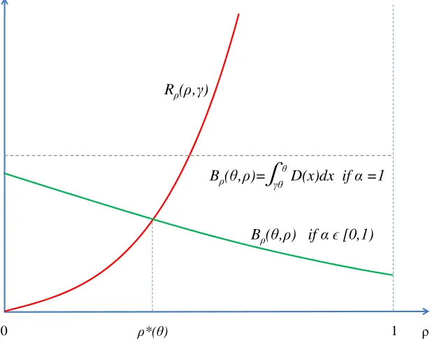
Figure 1 illustrates how to graphically obtain the optimal level of R&D activities,
ρ∗(θ), satisfying equation (37). Note that ifα 6= 1, the marginal benefit curveB
becomes the downward sloping curve in this figure. For this case, we find ρ∗(θ) at
the intersection of the marginal benefit and cost (green and red) curves. On the other hand, if α= 1, the regulated output function becomes independent of ρ, since ¯
qρ(.) = ¯q(.) = D(.). In this case, the marginal benefit curve becomes the (dotted)
horizontal line. Corollary 4 will later show (by proving the inequality Bρα(θ, .)>0)
that ρ∗(θ) is in a positive relationship with α, implying that the optimal level of
R&D activities in the caseα = 1 is higher than in the case α6= 1, as also apparent from Figure 1.
R ( , )
0 *( ) 1
[image:20.612.154.463.255.502.2]B ( , ) if [0,1) B ( , )= D(x)dx if =1
Figure 1. Observable R&D Choice of a Regulated Monopolist
Assumption 11-[ρ]. Under the regulated output function ¯qρ(.), production costs
are lower when R&D is successful than when it is not; i.e.,C(¯qρ(γθ), γθ)< C(¯qρ(θ), θ)
for all θ ∈(0, θ1].
Corollary 2. Let Assumptions 2-8 and 10 hold and Assumptions 9-[ρ] and 11-[ρ]
hold for allρ∈[0,1). Then, the optimal level of R&D activities, ρ∗(θ), is increasing
in θ ∈(0, θ1].
Interestingly, the above result implies that in regulatory environments where R&D activities increase productive efficiency, a less efficient monopolist always would always choose a higher level of R&D activities than a more efficient monopolist.
Now we can explore the dependence of ρ∗(θ) on the parameter γ. For this,
we need to estimate Bργ(θ, .), the response of the marginal benefit schedule to γ.
Unfortunately, the impact of γ on the partial derivative ¯qρ
ρ(.) appearing in the
first and third integrals of (35) is indeterminate because of the ambiguous effect of γ on the marginal informational cost function Gρ(.)/gρ(.) and its rate of change
∂[Gρ(θ)/gρ(θ)]/∂ρ. However, in situations where the welfare weightα is sufficiently
close to 1, the effect of these two terms on ¯qρ(.) and ∂q¯ρ(.)/∂ρ become negligible.
In such situations, the impact of γ on ρ∗(θ) can be predicted, provided that the
following assumption is also satisfied.
Assumption 12. Rρ,γ(ρ, γ) > 0 for all ρ ∈ [0,1) and γ ∈ (0,1) (marginal cost of
R&D activities is decreasing with the improvement level, i.e., increasing in γ).
Corollary 3. Let Assumptions 2-8 and 12 hold and Assumption 9-[ρ] hold for all ρ ∈ [0,1). If α is sufficiently close to one, then for all values of θ ∈ (0, θ], the optimal level of R&D activities, ρ∗(θ), is increasing with the improvement level, i.e.,
decreasing in γ ∈(0,1).
thanks to the resulting negligibility of the first and third integrals in (35), by the increase in the uncertain marginal benefit of R&D, i.e., Rθ
γθq¯
ρ(x)dx, through the
expansion of the range of integration [θγ, θ]. Thus, we expect the curve Bρ(θ, ρ) in
Figure 1 to shift up when γ decreases. On the other hand, the cost curve R(ρ, γ) would shift down under Assumption 12, yielding an increase inρ∗(θ).
In the next corollary, we show that when the social welfare is more equitable or the demand for the regulated product is higher, the monopolist will choose a higher level of R&D activities.
Corollary 4. Let Assumptions 2-8 and 10 hold and Assumption 9-[ρ] hold for all ρ ∈ [0,1). Then, for all values of θ ∈ (0, θ1], the optimal level of R&D activities, ρ∗(θ), is increasing in both α∈[0,1] and D0 ∈(0,∞).
It should be obvious from the optimal policy in (22)-(25) that the higher the welfare parameter α or the higher the maximal demand, D0, the higher will be marginal informational rent at each cost level, and consequently the higher will be the marginal benefit of R&D, implying a higher value for ρ∗(θ).
3.2
(Fully) Unobservable R&D
In this environment, R&D activities of the monopolist are unobserved by the regula-tor. So, we assume that the regulator, right before announcing the optimal regulatory policy, believes that the monopolist has not, so far, engaged in any R&D activities (ρ= 0) while it actually has (ρ >0). Resultingly, the binding beliefs of the regulator will be equal to her prior beliefs, i.e.,g0(.) =f(.), and the optimal regulatory policy
will behr,¯ p,¯ q,¯ s¯i, given by (13)-(16) calculated under the regulator’s prior beliefsf. The monopolist will exploit this situation involving asymmetric information about the value ofρ, as we will show below.
To simplify the rest of our analysis, we will suppose that Assumption 9-[0] holds, implying that ¯r(.) = 1. Now, let us fix θ ∈ (0, θ1] and γ ∈(0,1). When the level of
R&D activities is ρ, the profit expected by the monopolist can be written as
or simply
πe(θ, ρ) = B(ρ, γ)−R(ρ, γ) (39)
with
B(ρ, γ) =
Z θ1
θ
¯
q(x)dx+ρ
Z θ
γθ
¯
q(x)dx (40)
denoting the expected benefit of the monopolist. Differentiatingπe(θ, ρ) with respect
toρ yields
πe
ρ(θ, ρ) = Bρ(ρ, γ)−Rρ(ρ, γ) =
Z θ
γθ
¯
q(x)dx−Rρ(ρ, γ). (41)
Clearly,πe
ρ(θ,0)>0 and limρ↑1πρe(θ, ρ) =−∞.
The monopolist will choose a positive level of R&D activities (ρ >0) only if the resulting expected profits exceeds the profits under no activity (ρ= 0), i.e.,
πe(θ, ρ)≥πe(θ,0) (42)
or equivalently
ρ
Z θ
γθ
¯
q(x)dx−R(ρ, γ)≥0, (43)
usingR(0, γ) = 0 by Assumption 2. The above inequality requires that the expected additional informational rent is not below the average cost of R&D activities, i.e.,
Z θ
γθ
¯
q(x)dx≥ R(ρ, γ)
ρ . (44)
Using this last condition, the monopolist’s R&D problem can be written as follows:
max
ρ∈[0,1)π
e(θ, ρ) subject to (44). (45)
Proposition 4. Suppose that the R&D activities of the monopolist are unobservable. Let Assumptions 1-6 and 9-[0] hold. Then, for all θ ∈ (0, θ1], the optimal level of R&D activities, ρ∗(θ), for the monopolist is unique, lies in (0,1), and satisfies
Z θ
γθ
¯
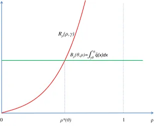
[image:24.612.154.462.324.577.2]q(x)dx=Rρ(ρ∗(θ), γ). (46)
Figure 2 illustrates how the optimal activity level ρ∗(θ) balances the marginal
benefit and marginal cost of R&D activities. Here, the marginal benefit curve is always horizontal unlike in Figure 1. In fact, this horizontal curve always lies above the varying marginal benefit curve in Figure 1. This will enable us to compare the optimal level of R&D activities in Sections 3.1 and 3.2, which we leave to Section 3.3.
q(x)dx
R ( , )
B ( , )=
0 *( ) 1
q(x)dx
Figure 2. Unobservable R&D Choice of a Regulated Monopolist
level of R&D activities negatively to the productive efficiency, is also valid when R&D activities are unobservable.
Corollary 5. Let Assumptions 1-6, 9-[0], and 11-[0] hold. Then, the optimal level of R&D activities, ρ∗(θ), is increasing in θ ∈(0, θ1].
Likewise, Corollary 6 will show that the inability of the regulator to observe the R&D activities of the monopolist has no effect on the direction of the relationship between the optimal level of R&D activities and several parameters of our model, involving γ, α, and D0.
Corollary 6. Let Assumptions 1-6, 9-[0]and 12 hold. Then, for all θ∈(0, θ1], the optimal level of R&D activities, ρ∗(θ), is increasing in α ∈ [0,1] and D0 ∈ (0,∞),
while decreasing in γ ∈(0,1) (or increasing in the improvement level).
3.3
Effect of Observability on the Monopolist’s R&D Choice
Now, we will explore how the presence of observability affects the level of R&D activities chosen by the monopolist. Basically, we will compare the values of ρ∗(θ)
calculated in Sections 3.1 and 3.2. This comparison will critically depend on whether the regulator weights the welfares of consumers and the monopolist equally or not.
Proposition 5. Let Assumptions 2-8 and 10 hold and Assumption 9-[ρ] hold for all ρ∈[0,1). Then for all θ ∈(0, θ1], the optimal level of R&D activities, ρ∗(θ), for
the monopolist is (i) independent of the observability of R&D if α = 1, (ii) lower when R&D activities are observable than when they are not if α ∈[0,1).
Part (i) of the above result stems from the observation that with α = 1, we have ¯qp(θ) = ¯q(θ) = D(θ). This implies that under Assumption 9-[0], the marginal
benefits of R&D are the same (as given by Bρ(θ, ρ) =
Rθ
γθD(x)dx) in Section 3.1
has lower values when R&D activities are observable than when they are not, i.e., ¯
qρ(.) < q¯0(.) = ¯q(.) for all ρ ∈ (0,1), also implying lower marginal benefits of
R&D under observability. (The dotted horizontal line in Figure 1 corresponds to the marginal benefit curve of unobservable R&D activities, which is always above the downward sloping marginal benefit curve of observable R&D activities.)
We should also note that Proposition 5, along with Propositions 3 and 4, im-plies that for each θ ∈ (0, θ1], the optimal level of R&D activities, ρ∗(θ), attains its
maximal level when α = 1, i.e., whenever the outcome under the Baron and Myer-son’s (1982) regulatory policy essentially boils down to the outcome under Loeb and Magat’s (1979) delegation scheme. The reason is that the monopolist in this par-ticular case is entitled to the whole social surplus under the original demand curve (within the range of possible marginal costs). Thus, the (constant) marginal benefit of investing in R&D will be at its highest level, implying that for any level of the marginal cost the optimal R&D choice will also be at its maximum.
Finally, our results in Section 3.1 and Section 3.2 also show that regardless whether R&D activities are observable or not, the optimal level of R&D activities,
ρ∗(θ), is increasing in θ,α and D0 and decreasing in γ.
3.4
Effect of Output Regulation on the Monopolist’s R&D
Choice
Finally, we will estimate the impact of output regulation on the monopolist’s R&D choice. For this, we have to calculate first the optimal level of R&D activities for the monopolist when the price and output of its product are not regulated.
Let us pick any θ ∈ (0, θ1]. One can easily verify that when the unregulated monopoly does not make any R&D, it would optimally choose the price and output of its product as pm(θ) = (D0 +D1θ)/2 and qm(θ) = (D0 −D1θ)/2, respectively.
Resultingly, the monopolist’s profit, πm(θ), would become
πm(θ) =pm(θ)qm(θ)−θqm(θ)−K = (D0−D1θ)2
4D1 −K. (47)
R&D is equal to
πm,e(θ, ρ) =ρπm(γθ) + (1−ρ)πm(θ)−R(ρ, γ), (48)
or simply
πm,e(θ, ρ) =B(θ, ρ)−R(ρ, γ), (49)
with
Bm(θ, ρ) = ρ(D0−D1γθ)2
4D1 + (1−ρ)
(D0−D1θ)2
4D1 −K (50)
denoting the expected benefit of the monopolist. The monopolist will choose a positive level of R&D activities (ρ >0) if and only if
πm,e(θ, ρ)−πm,e(θ,0)≥0 (51)
or equivalently
πm(γθ)−πm(θ)≥ R(ρ, γ)
ρ , (52)
using R(0, γ) = 0 by Assumption 2. Thus, the monopolist’s R&D problem can be written as
max
ρ∈[0,1)π
m,e
(θ, ρ), subject to (52). (53)
Noting that
πm,e
ρ (θ, ρ) = B
m
ρ (θ, ρ)−Rρ(ρ, γ)
= (1−γ)θ 2 D
(1 +γ)θ
2
−Rρ(ρ, γ) (54)
and
πm,eρρ (θ, ρ) =−Rρρ(ρ, γ), (55)
Proposition 6. Let Assumption 2-6 hold. If the price and output of the monopolist are not regulated, then for all θ ∈(0, θ1], the optimal level of R&D activities, ρm(θ),
for the monopolist is unique, lies in (0,1), and satisfies
(1−γ)θ
2 D
(1 +γ)θ
2
=Rρ(ρm(θ), γ). (56)
Using the characterizations provided by Propositions 4 and 6, we can compare the optimal R&D choice of a regulated monopolist whose R&D activities are unobservable to the optimal R&D choice of an unregulated monopolist, provided that the regulator treats the welfares of consumer and the monopolist sufficiently equally.
q(x)dx R ( , )
B ( , )=
0 m( ) 1
q(x)dx
[image:28.612.154.458.322.574.2]Bm( , ) = m( ) m( )
Figure 3. R&D Choice of an Unregulated Monopolist
then the optimal level of R&D activities for the monopolist is always higher when its price and output are regulated by the optimal policy (13)-(16) and its R&D activities are unobservable than when its price and output are not regulated at all. That is, ρ∗(θ) satisfying (46) is higher than ρm(θ) satisfying (56).
Figure 3 illustrates the above result graphically. (Apparently, the intersection of the dotted horizontal line, depicting the curve for the marginal benefits of unob-servable R&D activities, with the upward sloping marginal cost curve is above the optimal level of R&D activities, ρm(θ), chosen by an unregulated monopolist.) The
result in Proposition 7 is intuitive since in the extreme case where the regulator’s objective attaches equal weights to the welfares of consumers and the monopolist, the outcome of the regulatory incentive-compatible policy used in the monopoly mar-ket coincides with the outcome of the delegation scheme of Loeb and Magat (1979), which entitles the monopolist to the whole social surplus at the sold output. This surplus always exceeds the unregulated monopoly profit, offering higher incentives to the monopolist for investing in R&D when its production is regulated than when it is not.
On the other hand, in cases where the social welfare favors consumer welfare too much in relative to producer welfare (i.e., α is sufficiently small), it is not possible to compare the R&D choice of the regulated monopolist to that of the unregulated monopolist even in the simpler situation where R&D is unobservable. The reason is that under the regulatory policy (13)-(16), the adjusted demand schedule ¯q(.) affect-ing the informational rents of the monopolist nontrivially depends on the beliefs of the regulator through the inverse hazard rate functionF/f, whose range may involve any positive real. However, it is also obvious that the lower the weight parameterα
is, the higher will be the effect of the inverse hazard rate on the quantity schedule. In other words, the lower the parameterα, the more suppressed the marginal benefit curve of the regulated monopolist, implying that the difference ρ∗(θ)−ρm(θ) will
4
Conclusion
In this paper we have considered a monopolist with unknown marginal costs and studied whether the incentive-compatible mechanism of Baron and Myerson (1982), which optimally regulates the price and output of the monopolistic product, can pro-vide sufficiently large incentives to the monopolist to make cost-reducing innovations through R&D. The R&D technology the monopolist has access to is defined by the improvement and probability parameters. The improvement parameter that is given to the monopolist measures the reduction in the marginal cost if R&D becomes suc-cessful. On the other hand, the probability parameter which is directly controlled by the monopolist through its R&D activities measures the success likelihood of R&D. While we let the monopolist in our model to freely choose the level of its R&D activities, we allow for an environment where realised R&D level is observable by the regulator as well as an environment where it is not. For both environments, we characterize the optimal level of R&D activities chosen by the monopolist as well as conditions ensuring that the optimal level is unique and positive. Irrespective of the observability of R&D, we find that the optimal level of R&D activities is higher when the monopolist is productively less efficient, provided that R&D activities al-ways increase productive efficiency. In addition, the improvement level of R&D, the maximal size of demand and the relative weight of the monopolist welfare have, all, positive impacts on the optimal level of R&D activities.
reducing the marginal benefit of R&D.
References
Arrow, K.J., 1959. “Economic Welfare and the Allocation of Resources for Inven-tion,” The Rand Corporation, rand Paper P-1856- RC. Republished as: “Economic Welfare and the Allocation of Resources to Invention,” in R. R. Nelson (ed.), The Rate and Direction of Economic Activity, Princeton University Press, N.Y., 1962.
Baron, D. and Myerson, R.B., 1982. “Regulating a Monopolist with Unknown Costs,”Econometrica 50, 911-930.
Crew, M.A. and Kleindorfer, P. R., 1986. The Economics of Public Utility Regula-tion. Cambridge, MA: MIT Press.
Dasgupta, P.S., Hammond, P. J., and Maskin, E.S., 1979. “The Implementation of Social Choice Rules: Some Results on Incentive Compatibility,”Review of Economic Studies46, 185-216.
Dupuit, J., 1952. “On the Measurement of the Utility of Public Works,” Interna-tional Economics Papers2, 83-110 (translated by R. H. Barback from ”de la Mesure de l’Utilite des Travaux Publics,” Annales des Ponts et Chaussees, 2nd Series, Vol. 8, 1844).
Giuseppe, C., and Vincenti, C.D., 2004. “Can Price Regulation Increase Cost-Efficiency?,”Research in Economics 58(4), 303-317.
Harris, M., and Townsend, R.M., 1981. “Resource Allocation under Asymmetric Information,” Econometrica 49, 33-64.
Koray, S., and Saglam, I., 2005. “The Need for Regulating a Bayesian Regulator,”
Journal of Regulatory Economics 28, 5-21.
Undesirable?,” Economics Bulletin 3(12), 1-10.
Koray, S. and Sertel, M.R., 1990. “Pretend-but-Perform Regulation and Limit Pricing,”European Journal of Political Economy 6, 451-72.
Laffont, J. J., 1994. “The New Economics of Regulation Ten Years After,”
Econometrica 62, 507-37.
Lewis, T.R., and Yildirim, H., 2002. “Learning by Doing and Dynamic Regulation,”
The Rand Journal of Economics33(1), 22-36.
Loeb, M., and Magat, W.A., 1979. “A Decentralized Method for Utility Regulation,”
Journal of Law and Economics 22, 399-404.
Myerson, R.B., 1979. “Incentive Compatibility and the Bargaining Problem,”
Econometrica 47, 61-74.
Sappington, D., 1982. “Optimal Regulation of Research and Development under Imperfect Information,”The Bell Journal of Economics 13(2), 354-368.
Vogelsang, I., 1988. “A Little Paradox in the Design of Regulatory Mechanisms,”
International Economic Review29, 467-76.
Appendix
Proof of Proposition 1. See pages 920-921 of Baron and Myerson (1982).
Proof of Lemma 1. Pick any ρ ∈[0,1). Assumption 7 ensures that Gρ(θ)/gρ(θ)
is increasing in θ ∈(0, θ1] if θ 6=γθ1. One can also check that
Gρ(γθ1)
gρ(γθ1) −θlim↓γθ1
Gρ(θ)
gρ(θ) =
−f(θ1)F(γθ1)−(1−ρρ)f(θ1)
f(γθ1)hf(θ1) + γ(1ρ−ρ)f(γθ1)i
completing the proof.
Proof of Proposition 2. Directly obtained by mimicking the proof of Proposition
1 (thanks to Lemma 1).
Proof of Lemma 2. Differentiating (20) with respect to ρyields
∂[Gρ(θ)/gρ(θ)]
∂ρ =
F(θ/γ)f(θ)− 1
γF(θ)f(θ/γ)
[ρf(θ/γ) + (1−ρ)f(θ)]2 if 0< θ≤γθ1,
1
(1−ρ)2f(θ) if γθ1 < θ≤θ1.
(58)
The second line of the above derivative is always positive. Rewriting Assumption 8 for any θ ∈ (0, γθ1] as F(θ)/f(θ) < γF(θ/γ)/f(θ/γ), we obtain that the first line of (58) is positive, as well. This proves that Gρ(θ)/gρ(θ) is increasing in ρ. Also,
∂[Gρ(θ)/gρ(θ)]/∂ρis nondecreasing in ρ, by Assumption 7.
Proof of Corollary 1. Directly obtained from equations (22) and (23), given
Lemma 2.
Proof of Remark 1. By Assumption 9-[0], Assumption 10 holds if (36) is satisfied. Pick any θ ∈ (0, θ1]. We have ¯q0(θ) = ¯q(θ) and therefore,
Rθ
γθq¯
0(x)dx=Rθ
γθq¯(x)dx, which is always positive, by equations (13) and (14). Now,
let α = 1. For all ρ ∈ [0,1), ¯qρ(θ) = ¯q(θ) = D(θ), implying ∂q¯ρ(θ)/∂ρ = 0. Thus,
Bρ(θ,0) =
Rθ
γθq¯(x)dx >0. Since both ¯q
ρ(.) and ¯qρ
ρ(.) are continuous in α, (36) holds
for all α∈[0,1] which are sufficiently close to 1.
Proof of Lemma 3. Pick any θ ∈ (0, θ1] and ρ ∈ [0,1). Since Assumption 9-[ρ] holds, Bρ(θ, ρ) is given by (35). Differentiating Bρ(θ, ρ) with respect to ρ yields
Bρ ρ(θ, ρ) =
Z θ1
θ
¯
qρ
ρρ(x)dx+ 2
Z θ
γθ
¯
qρ
ρ(x)dx+ρ
Z θ
γθ
¯
qρ
ρρ(x)dx. (59)
First letα∈[0,1). Thanks to Assumptions 7 and 8, we have ¯qρ
1, and
¯
qρρρ (θ) = D
′
(¯pρ(θ))(1−α)∂
2(Gρ(θ)/gρ(θ))
∂ρ2 ≤0, (60)
by Lemma 2. Therefore, Bρρ(θ, ρ) < 0. Now let α = 1. Then, we have
qρ(.) = ¯q(.) = D(.), implying B
ρρ(θ, ρ) = 0. Thus, for all α ∈ [0,1], we have
Bρρ(θ, ρ) ≤ 0. Moreover, we have Rρ ρ(θ, ρ) > 0 by Assumption 6, implying
πe
ρ ρ(θ, ρ)<0.
Proof of Proposition 3. Pick any θ ∈ (0, θ1]. By Proposition 2 (thanks to As-sumption 7), the optimal regulatory policy is given by (22)-(25). Note from equations (34) and (35) that under Assumption 9-[ρ], equation (37) is the first order condition for the problem in (33). Assumption 5 implies that ρ∗(θ) <1. On the other hand,
Assumptions 3-5 along with Assumption 10 and the continuity ofπe(θ, ρ) in ρimply
that ρ∗(θ)>0.
Now, pick any ρ ∈ [0,1) and note that πe
ρ ρ(θ, ρ) < 0 by Lemma 3 (thanks to
Assumptions 6-8 and 9-[ρ]). Thus, ρ∗(θ) satisfies the second-order condition and it
is unique.
Finally, note that Assumptions 4 and 10 implyπe
ρ(θ,0)>0, while the continuity
of Bρ(θ, ρ) and Rρ(ρ, γ) with respect to ρ imply that πeρ(θ, ρ) is continuous in ρ.
Since we have already found thatρ∗(θ) is the unique maximizer ofπe(θ, ρ) among all
ρ∈[0,1), we must have πe(θ, ρ∗(θ))−πe(θ,0)>0, ensuring the feasibility condition
(32).
Proof of Corollary 2. Pick anyθ ∈(0, θ1]. Since Assumptions 2-8 and 10 hold and Assumption 9-[ρ] holds for allρ ∈[0,1), Proposition 3 ensures that ρ∗(θ) is unique,
lies in (0,1), and satisfies πe
ρ(θ, ρ∗(θ)) = 0 as in (37). Now, pick any ρ ∈ [0,1). By
Assumption 9-[ρ], Bρ(θ, ρ) is given by (35). Differentiating (35) with respect to θ
yields
Bρ θ(θ, ρ) = ¯qρ(θ)−γq¯ρ(γθ) +ρ
¯
qρ
ρ(θ)−q¯ ρ ρ(γθ)
−q¯ρ
ρ(θ)
= ¯qρ(θ)−γq¯ρ(γθ) + (ρ−1)¯qρ
ρ(θ)−ρq¯ ρ
ρ(γθ). (61)
First letα∈[0,1). By Corollary 1 (thanks to Assumptions 7 and 8), ¯qρ
ρ(θ)<0. Now
let α = 1. Then ¯qρ
¯
qρ
ρ(θ) ≤ 0. On the other hand, by Assumption 11-[ρ], it is true that C(¯qρ(θ), θ) >
C(¯qρ(γθ), γθ), or equivalently ¯qρ(θ) > γq¯ρ(γθ). Therefore, B
ρ θ(θ, ρ) > 0, implying
πe
ρ θ(θ, ρ) > 0 since Rρ θ(ρ, γ) = 0. Additionally, for all ρ ∈ [0,1], πρ ρe,ρ,γ(θ) < 0 by
Lemma 3 (thanks to Assumptions 6-8 and 9-[ρ]). Sinceπe
ρ(θ, ρ∗(θ)) = 0, ρ∗(θ) must
be increasing inθ ∈(0, θ1].
Proof of Corollary 3. Pick any θ∈(0, θ1]. Assumption 9-[0] implies Assumption 10. Since Assumptions 2-8 and 10 hold and Assumption 9-[ρ] holds for allρ∈[0,1), Proposition 3 ensures thatρ∗(θ) is unique, lies in (0,1), and satisfies πe
ρ(θ, ρ∗(θ)) = 0
as in (37). Now, pick anyρ∈[0,1). First, letα= 1. From equations (22), (23), and (24) it follows that ¯qρ(θ) = ¯q(θ) = D(θ), hence ¯qρ
ρ(θ) = 0 for all θ ∈ (0, θ1]. Since
Assumption 9-[ρ] holds, ¯rρ(θ) = 1 for all θ ∈ (0, θ1]. Thus, equation (35) implies
Bρ(θ, ρ) =
Rθ
γθq¯(x)dx. It follows thatBρ γ(θ, ρ) =−θq¯(γθ)<0; implying π e
ρ γ(θ, ρ) =
−θq¯(γθ)−Rρ γ(ρ, γ)<0 by Assumption 12. Moreover, for allρ∈[0,1), πρρe (θ, ρ)<0
by Lemma 3 (thanks to Assumptions 6-8 and 9-[ρ]). Since πe
ρ(θ, ρ∗(θ)) = 0, ρ∗(θ)
must be decreasing in γ ∈(0,1).
Finally, since Bρ γ(θ, ρ) is continuous in α and the differences ¯qρ(.)−q¯(.) and
¯
qρ
ρ(.)−q¯ρ(.) = ¯qρρ(.) are negligible when 1−α is sufficiently small, the above result
obtained for α= 1 is also true for allα ∈[0,1] which are sufficiently close to 1.
Proof of Corollary 4. Pick anyθ ∈(0, θ1]. Since Assumptions 2-8 and 10 hold and Assumption 9-[ρ] holds for allρ ∈[0,1), Proposition 3 ensures that ρ∗(θ) is unique,
lies in (0,1), and satisfiesπe
ρ(θ, ρ∗(θ)) = 0 as in (37). Now, pick any ρ ∈[0,1). Since
Assumption 9-[ρ] holds, ¯rρ(θ) = 1 for all θ ∈ (0, θ1]. It follows from (22) and (23)
that ¯qρ(θ) is increasing in both α ∈[0,1] and D0 ∈(0,∞). Moreover, we have
∂2q¯ρ(θ)/∂ρ∂α =−D′(¯pρ(θ))∂(Gρ(θ)/gρ(θ))/∂ρ >0 (62)
and
∂2q¯ρ(θ)/∂ρ∂D0 = 0. (63)
Then, it follows from (35) that Bρ α(θ, ρ) > 0 and BρD0(θ ρ) > 0, implying
πe
ρ α(θ, ρ) > 0 and πρDe 0(θ, ρ) > 0. Moreover, for all ρ ∈ [0,1), π
e,ρ,γ
Lemma 3 (thanks to Assumptions 6-8 and 9-[ρ]). Sinceπe
ρ(θ, ρ∗(θ)) = 0, ρ∗(θ) must
be increasing in both α∈[0,1] and D0 ∈(0,∞).
Proof of Proposition 4. Pick any θ ∈ (0, θ1]. By Assumption 1, the optimal regulatory policy is given by (13)-(16). Assumption 9-[0] implies that ¯r(.) = 1. Then, (46) is the first order condition for the problem in (45). The marginal benefit of R&D activitiesRθ
γθq¯(x)dxis always positive by (13), and (14). Then, Assumptions
3 and 4 imply ρ∗(θ) > 0, whereas Assumption 5 implies ρ∗(θ) < 1. On the other
hand, Assumptions 2 and 6 together imply that Rρ(ρ∗(θ), γ) > R(ρ∗(θ), γ)/ρ∗(θ);
so (44) is satisfied at ρ∗(θ). Finally, the second order condition holds, since
πe
ρρ(θ, ρ) =−Rρρ(ρ, γ)<0 by Assumption 6. This also ensures thatρ∗(θ) is unique.
Proof of Corollary 5. Pick any θ ∈(0, θ1]. Since Assumptions 1-6 and 9-[0] hold, Proposition 4 ensures thatρ∗(θ) is unique, lies in (0,1), and satisfies πe
ρ(θ, ρ∗(θ)) = 0
as in (46). By Assumption 1, the optimal regulatory policy is given by (13)-(16). Assumption 9-[0] implies that ¯r(.) = 1. Now pick any ρ ∈ (0, θ1]. Differentiating (41) with respect toθ yields
πe
ρ θ(θ, ρ) = ¯q(θ)−γq¯(γθ), (64)
which is always positive, since γ < 1, Assumption 11-[0] holds, and ¯q(.) is de-creasing by (13) and (14), thanks to Assumption 1. Moreover, for all ρ ∈ [0,1),
πe
ρρ(θ, ρ) = −Rρρ(ρ, γ) < 0 by Assumption 6. Since πρe(θ, ρ∗(θ)) = 0, ρ∗(θ) must be
increasing inθ ∈(0, θ1].
Proof of Corollary 6. Pick any θ ∈(0, θ1]. Since Assumptions 1-6 and 9-[0] hold, Proposition 4 ensures thatρ∗(θ) is unique, lies in (0,1), and satisfies πe
ρ(θ, ρ∗(θ)) = 0
as in (46). By Assumption 1, the optimal regulatory policy is given by (13)-(16). Assumption 9-[0] implies that ¯r(.) = 1. Now pick any ρ ∈ (0, θ1]. Differentiating (41) with respect toγ yields
πe